Proceeding Paper

Prediction of Cooling Energy Consumption Using a Neural Network on the Example of the Hotel Building †

Faculty of Mining and Geoengineering, AGH University of Science and Technology, 30-059 Kraków, Poland
*
Author to whom correspondence should be addressed.
Presented at the First World Energies Forum, 14 September–5 October 2020; Available online: https://wef.sciforum.net/.
Proceedings 2020, 58(1), 21; https://doi.org/10.3390/WEF-06917
Published: 11 September 2020
(This article belongs to the Proceedings of The First World Energies Forum—Current and Future Energy Issues)

Abstract

:
The purpose of this work is to determine internal and external factors affecting the cooling energy demand of a building. During the research, the impact of weather conditions and the level of hotel occupancy on cooling energy, which is necessary to obtain indoor comfort conditions, was analyzed. The subject of research is energy consumption in the Turówka hotel located in Wieliczka (southern Poland). In the article, the designer of neural networks was used in the Statistica statistical package. To design the network, a widely used multilayer perceptron model with an algorithm with backward error propagation was used. Based on the collected input and output data, various multilayer perceptron (MLP) networks were tested to determine the relationship most accurately reflecting actual energy consumption. Based on the results obtained, factors that significantly affect the consumption of thermal energy in the building were determined, and a predictive energy demand model for the analyzed object was presented. The result of the work is a forecast of cooling energy demand, which is particularly important in a hotel facility. The prepared predictive model will enable proper energy management in the facility, which will lead to reduced consumption and thus costs related to facility operation.

1. Introduction

The advancement of civilization and the development of society increase the amount of time that a person spends indoors. Currently, in developed countries, people spend up to 80–90% of their lives in buildings, which is why it is so important to ensure proper conditions and high indoor air quality. In new buildings’ heating, ventilation and air-conditioning systems play a crucial role due to high user comfort requirements. However, air treatment processes are very expensive, while the removal of heated air in winter causes the process itself to be unprofitable. The main tasks of designers in recent times are to reduce heating and cooling energy consumption through the use of devices and systems with higher efficiency, and to reduce energy losses during energy distribution, as well as through proper management of systems. The forecasting of energy consumption in a building is particularly important in terms of planning, managing, and optimizing energy systems. Accurate and reliable heating and cooling energy forecasts for buildings can bring significant benefits to energy savings. The forecasting heating energy consumption is a difficult task due to numerous disturbances and deviations from observed trends. In the case of facilities such as a hotel, the demand for cooling and heating energy, in addition to meteorological factors, is determined by the hotel occupancy and user activity (the use of facilities on the premises, e.g., swimming pool, restaurant, conference room, etc.).
Building energy consumption prediction is crucial to appropriate energy management and, subsequently, to improve the energy efficiency of systems and performance of the buildings. In general, methods for estimating and modeling energy consumption could be divided into two groups: engineering and data-driven approaches. The first type uses physical and thermodynamic functions to evaluate the energy consumption of the building or system. A data-driven approach defines the relationship between energy consumption and identified factors based on historical data [1]. In recent years, artificial intelligence methods have become very popular. This technique is often applied to the prediction of energy consumption due to good accurate prediction results. Among the most popular data-driven prediction models using the empirical approach are artificial neural networks (ANNs) and support vector machines (SSM) [2].
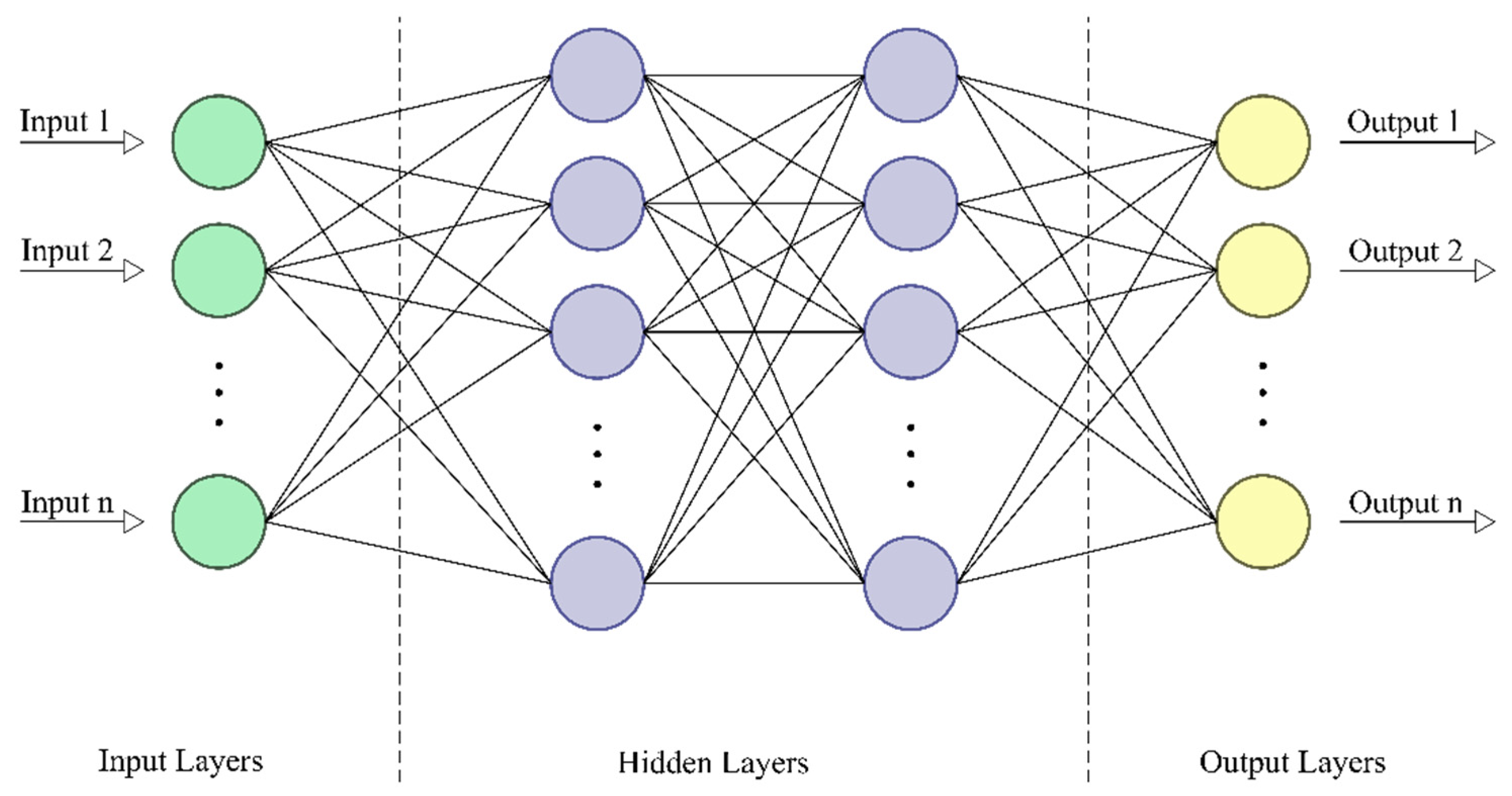
Artificial neural networks consist of three types of layers: input (this collects data and passes them on), hidden (connections between neurons are searched for here, i.e., the learning process takes place) and output (this collects conclusions and analysis results). A neural network can consist of any number of layers. Unprocessed data goes into the first layer. Each subsequent layer receives data resulting from the processing of data in the previous layer. What the last layer produces is the so-called system output [3]. The simplified artificial neural network was proposed for the first time by McCulloch and Pitts in 1943 [4]. A schematic diagram of the multilayer feedforward neural network architecture is shown in Figure 1.
There are many types of artificial neural networks (ANN), including the backpropagation network (BPNN), the general regression neural network (GRNN), and the radial basis function network (RBFN) [3]. The most commonly used neural network architecture today is the multilayer perceptron (MLP). Each neuron calculates the weighted average of the inputs to it, and calculates the result using the transition function f and gives it to the output. There is also a shift component in each layer of MLP network neurons. Choosing the right number of hidden layers and the number of neurons present in them is an important aspect for a perceptron. The choice of activation function and network learning method is also significant.
Numerous interesting methods of prediction of building energy consumption have been described in the literature [5,6,7]. Nowadays, widely used solutions are data-driven models applied to estimate electricity consumption in buildings and to analyze energy consumption patterns [8,9,10,11,12,13,14]. As many studies [15,16,17] show, artificial neural networks could be useful also in the prediction of heating and cooling energy consumption. Zhao et al. [18] investigated the energy consumption of a variable refrigerant volume system in the office building. The authors compared three types of prediction models: ANN, SVM, and ARIMA (autoregressive integrated moving average). The results showed that the ANN model is better than the other two types. In their paper, Biswas et al. [19] proposed a prediction model of residential building energy consumption. The input variables included the number of days, outdoor temperature, and solar radiation. The output variables are building and heat pump energy consumption. In a paper by Pino-Mejías et al. [20], the authors presented prediction models of the heating and cooling energy demands, energy consumptions, and CO2 emissions for office buildings in Chile. The study shows that multilayer perceptron provides a satisfactory degree of accuracy in the determination of demand, consumption, and CO2 emissions. Annual energy consumption by heating, ventilation, air conditioning (HVAC) systems was also predicted by Nasruddin et al. [21]. The authors used ANN model with the range of decision variables including cooling setpoint, supply airflow rate, window area, supply air temperature, etc. A university building was the subject of the study. The result showed that optimization of HVAC improvement influenced both thermal comfort as well as annual energy consumption.
This paper presents an integrated approach to predict energy consumption and develop a predictive model using an artificial neural network. The study includes an analysis of the energy consumption of cooling systems based on the meteorological data and historical cooling energy data during the summer season. The main purpose is to create an accurate ANN model for the Turówka hotel to estimate daily cooling energy consumption. The cooling system in the hotel is accountable for about 50–60% of the total building energy consumption; therefore, the study focused only on the cooling demand [22].

2. Methods and Building Description

The building studied in this paper is the Turówka hotel, located in Wieliczka, the south-central part of Poland near Kraków. It is the reconstruction of a historic salt store of 1812, which is entered into the register of historical monuments. The building is under preservation maintenance, thus, during hotel refurbishment of old saltworks and hotel adaptation, the mass and dimension of the building should stay the same. The used building materials and window and door frames were selected with the aim of recreating the structure as faithfully as possible. The building includes four overground floors and a basement, with the hotel section possessing a useable floor area of 5525.00 m2 and a capacity of 19,300 m3. The hotel has 50 double rooms, a restaurant for 90 people, a hotel bar for 30 people, a drink bar for 30 people, a conference room for 40 people and a pool. Central heating installation is powered by two low-temperature gas boilers with a capacity of 250 and 350 kW. Currently, the hotel uses a two-pipe central heating system with panel radiators and thermostatic valves. The domestic hot water is prepared in the gas boiler house with circulation and with heating circulation pump control. The building is equipped with mechanical supply and exhaust ventilation carried out by seven air-handling units with rotary exchangers, and air-handling units for the kitchen with an exchanger using glycol. The coolers in the air-handling unit (AHU) are supplied with chilled water at 8 °C/14 °C temperature parameters. The same cooling installation also supplies fan coil units located in the hotel rooms and other rooms intended for guests. The hotel building and its immediate surroundings are shown in Figure 2.
Cooling energy meters have been installed in main system areas, i.e., feed and return of the high and, depending on demand, low parameters of the refrigerant. Data are transmitted via a serial communications protocol—MODBUS RTU—and stored in a recording system. Measurements are made using MULTICAL heat meters by Kamstrup. To ensure measurement stability, flow sensors were submitted to a type approval according to EN 1434 [24], which includes the 2400 h measurement stability test of flow sensors.
This paper includes an analysis of the cooling energy consumption of the hotel. In the summer season, the main building operating costs are related to the cooling system, which ensures thermal comfort for users. Due to the prevailing share of cooling energy demand in total energy consumption in the summer season, the research was focused on providing the most accurate model for the prediction of cooling energy consumption. The data analyzed in this study are a daily time series collected from 15 May to 15 September 2019. This period is a summer season in Poland when the hotel cooling system is in operation. The data include cooling energy consumption in the building. The outside temperature was measured directly at the hotel area. Other meteorological data are obtained from the National Research Institute—Polish Institute of Meteorology and Water Management.
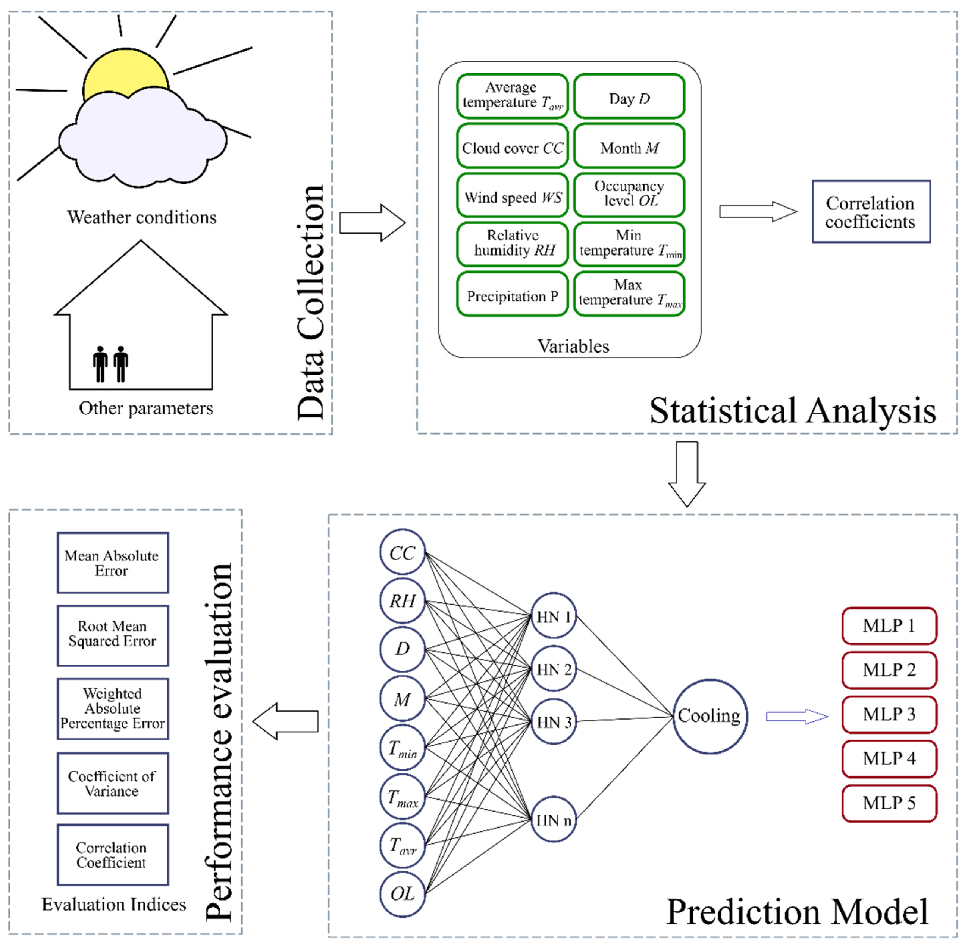
The study has been divided into four parts. Firstly, the data, including meteorological data and data from the analyzed building, were collected. Another step was to examine the relationship between cooling energy demand and the identified variables in the analyzed period. On this basis, the factors that may affect energy consumption were selected. Due to the minimal impact of some factors as well as the practical approach to the application of prediction algorithms, only the most significant ones are most often used. Among ten variables, namely, day, month, occupancy level, average outside temperature, minimum temperature, maximum temperature, relative humidity, cloud cover, precipitation, and wind speed, the last two parameters were rejected. In the paper, a simplified data-driven model for the prediction the energy consumption is presented. An ANN-based model was used to predict the cooling energy used in a building in the summer season. Figure 3 illustrates the research process.
In this study, three evaluation indices are used to measure the performance of the proposed approach, including the mean absolute error (MAE), root mean squared error (RMSE), and coefficient of variance (CV) [16,18,25]. Additionally, the weighted absolute percentage error (WAPE), proposed by other authors, was used [26]. The mathematical representation of indicates are represented in Equations (1)–(4):
M A E = 1 n i = 1 n | E A E P |
R M S E = 1 n i = 1 n ( E A E P ) 2
C V = 1 n i = 1 n ( E A E P ) 2 E A ¯
W A P E = i = 1 n | E A E P | i = 1 n E A
where n denotes the entire number of observations, E A is the actual value, E A ¯ denotes the mean of actual values, and E P represents the predicted value.

3. Results

3.1. Preliminary Statistical Analysis

To increase the accuracy of the prediction, the pre-selected meteorological values and data related to the use of the building were subjected to basic statistical analysis. During the initial analysis, ten parameters were identified that may affect the cooling load, including the day of the week, month, the minimal and maximum outside temperature during the day, average daily temperature, occupancy level, average daily cloud cover, wind speed, relative humidity, and precipitation. Statistical analysis was performed for the data presented in Table 1.
Table 2 presents descriptive statistics for each analyzed variable. Day and month are listed, but statistics are not provided for them because these parameters represent categorical variables in the model.
The analysis was based on the Pearson correlation coefficients between the studied variables and the predicted output. The results are summarized in Table 3.
Based on the results in the table, it was decided that in further analysis, the wind speed and precipitation parameters, which showed the smallest relationships with the searched value, would be rejected. Despite the low correlation coefficient between cooling energy demand and occupancy level, this variable was accepted for further consideration due to individual cooling control in guest rooms.
A regression graph with histograms presenting the relationship between energy consumption and the average temperature was plotted (Figure 4a). The data were ordered and divided into groups in specified temperature ranges. Having removed outliers and extremes, linear relationships were plotted in the form of box plots (Figure 4b).
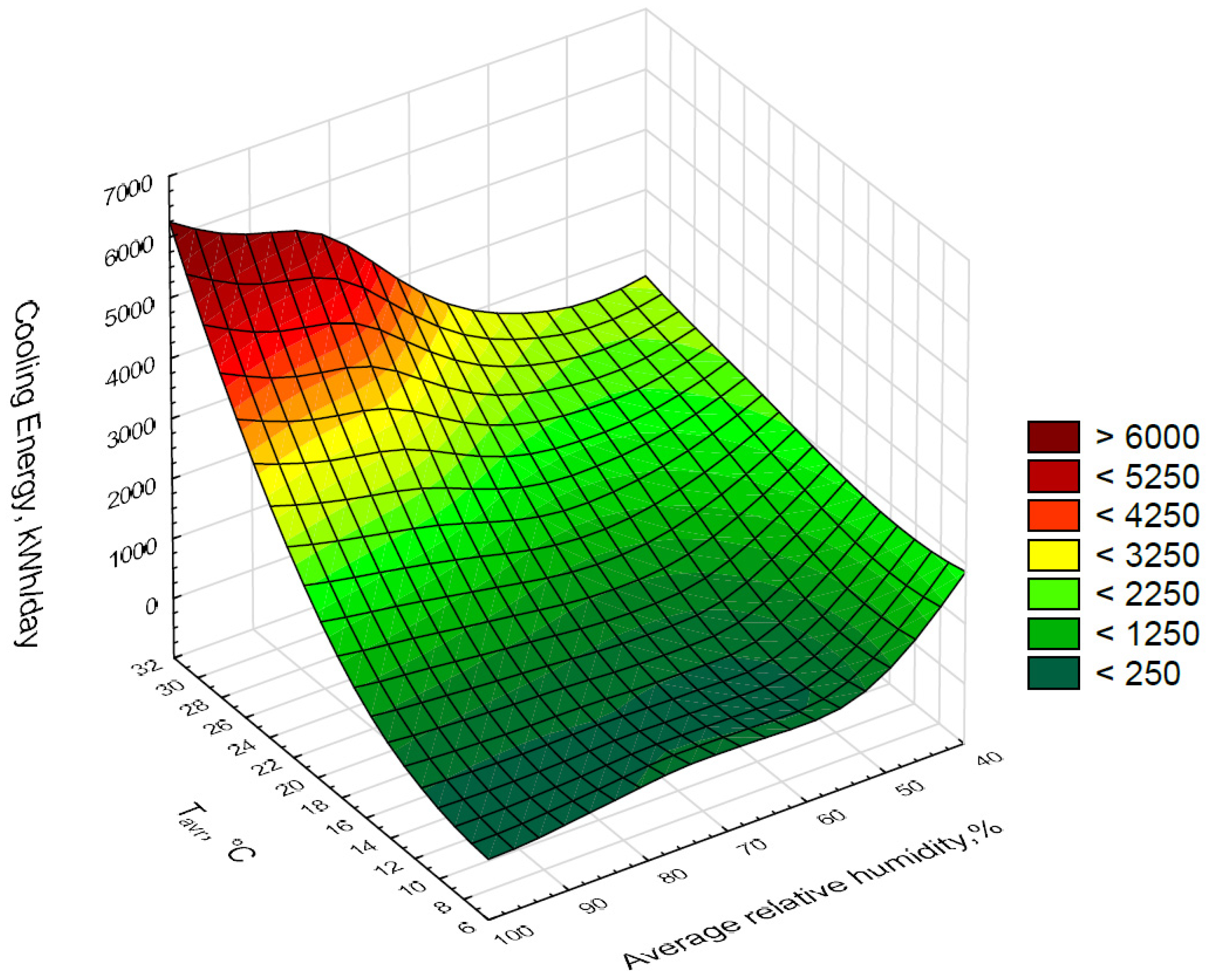
The next step was to investigate the relationship between energy consumption for cooling and the two variables with the highest correlation coefficients: average temperature and relative humidity. The diagram for the cooling system is shown in Figure 5.

3.2. Neural Networks

The Statistica Artificial Neural Network Package was used to prepare a predictive model. Multilayer perceptrons with backpropagation were performed. The number of hidden neurons, the hidden layer activation functions, and the output layer activation function are selected using the methodology based on statistical tests and least-squares estimation. Five different networks were created by combining four types of activation functions and a different number of hidden neurons. The BFGS (Broyden–Fletcher–Goldfarb–Shanno) training algorithm was chosen for this work. Based on the correlation coefficient, five models were selected, and these are described in Table 4.

3.3. Performance of the Model

Based on the above-mentioned indicators, namely, MAE, RMSE, WAPE, CV, and correlation coefficient (R2), selected models were compared. The results for cooling consumption are presented in Table 5.
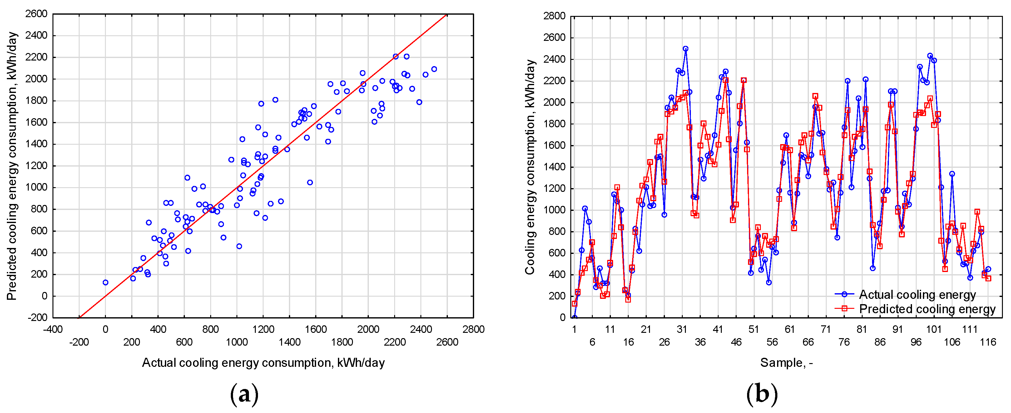
For each of the analyzed outputs, the MLP 5 model was the most accurate in modeling energy consumption for the full dataset. Further analysis was therefore carried out only for this model. Figure 6 shows the comparison between actual consumptions and forecasts for the cooling system.

4. Discussion

In this paper, the ANN predictive model for hotel Turówka is presented. The CV rate for the proposed models varies from 19.55% to 19.88%. Similarly, the weighted absolute percentage error for models ranged from 15.53% to 16.49%, and the correlation coefficient in range of 0.924–0.926. Based on these investigated indicators for each of the analyzed systems, the MLP 5 model was selected. The differences between the proposed models are not large, and the choice was conditioned mainly by lower values of the coefficients describing the prediction error. For model 5, mean absolute error was 189 kWh/day, and weighted absolute percentage error was 15.53%. The predicted results are found to be very close to the experimental values. For maximum and minimum values of energy consumption, the largest differences between the actual value and predicted value are visible.
Table 6 presents sensitivity coefficients, which describe the change in the system’s outputs due to variations in the parameters that affect the system. For each of the analyzed models, the ratio of network error without a given variable to the error with a set of inputs was given. A quotient of less than 1 means that the network works even better without a given variable, which is an obvious signal to remove a given independent variable from the analysis.
As Table 6 shows, the impact of variables on predicted value varies depending on the analyzed model. As mentioned before, the MLP 5 model was chosen for further analysis, for which the most important parameters are the minimum and maximum temperatures during the day. The occupancy level does not affect the values obtained. During the initial analysis, attention was paid to the relationship between the consumption of cooling energy and relative humidity. As the analysis shows, humidity is included in the model, but it is not a determining factor. The sensitivity factor smaller than 1 in model MLP 1 suggests that this parameter is not important in analysis. This is also due to the significant correlation between temperature and humidity (Table 3).

5. Conclusions

The HVAC system consumes a large amount of energy, especially in commercial buildings. Energy consumption prediction is an interesting solution for energy management building, and hence for saving energy and reducing operational costs. The cooling load is affected by many factors, including weather conditions, building operation, thermal performance, and users’ behavior. In this paper, a simplified data driven-model for predicting energy consumption has been presented. The methodology is based on the use of artificial neural networks. A sensitivity analysis demonstrated that part of the proposed input variables initially selected offer limited contribution to the model. Among the ten identified parameters, eight input features were used in the proposed models. Based on the mentioned variables, five ANN models were created and compared using the evaluation coefficients discussed above. Model MLP 5, with six hidden neurons, was chosen as the most appropriate and effective. External minimum, average, and maximum temperature as well as relative humidity were considered the most important variables in this selected model. Cloud cover, day, and month have less impact on the predicted values. Based on the sensitivity analysis, it was found that the occupancy level has no significant effect on the prediction model. For each of the output parameters, the predictions were good, especially in terms of average values. The biggest errors were noticeable for extreme values that are not completely reproduced by the model. The largest observed difference in the analyzed period was 596 kWh/day, which was 25% of the actual value. The best mapping was obtained for cooling energy. This is particularly important due to the prevailing share of cooling energy in the total energy load of the building during the summer period. The prediction task performed for the whole day is difficult due to changing conditions. To increase the accuracy of predictive models, the analysis could be performed based on hourly energy consumption.
Author Contributions

Conceptualization, M.B. and K.Z.; methodology, M.B.; software, K.Z.; validation, M.B.; formal analysis, M.B.; investigation, K.Z.; resources, K.Z.; data curation, K.Z.; writing—original draft preparation, K.Z.; writing—review and editing, M.B.; visualization, K.Z.; supervision, M.B.; project administration, M.B. All authors have read and agreed to the published version of the manuscript.

Funding

This research was funded by the European Regional Development Fund, Intelligent Development Program, grant number POIR.01.01.01-00-0720/16.

Conflicts of Interest

The authors declare no conflict of interest.

Nomenclature

CCCloud cover, -
DDay of the week, -
EAActual value of the energy consumption, kWh/day
EPPredicted value of the energy consumption, kWh/day
MMonth, -
nNumber of observations, -
OLOccupancy level, %
PPrecipitation, mm
R2Correlation coefficient
RHDaily average relative humidity, %
TminDaily minimum temperature, °C
TmaxDaily maximum temperature, °C
TavrDaily average temperature, °C
AHUAir Handling Unit
ANNArtificial Neural Network
ARIMAAutoregressive, Integrated and Moving Average
BFGSBroyden-Fletcher-Goldfarb-Shanno
BPNNBack Propagation Neural Network
CVCoefficient of Variance
GRNNGeneral Regression Neural Network
HVACHeating, Ventilation, Air Conditioning
MAEMean Absolute Error
MLPMultilayer Perceptron
RBFNRadial Basis Function Network
RMSERoot Mean Squared Error
SSMSupport Vector Machine
WAPEWeighted Absolute Percentage Error

References

  1. Benedetti, M.; Cesarotti, V.; Introna, V.; Serranti, J. Energy consumption control automation using Artificial Neural Networks and adaptive algorithms: Proposal of a new methodology and case study. Appl. Energy 2016, 165, 60–71. [Google Scholar] [CrossRef]
  2. Wei, Y.; Zhang, X.; Shi, Y.; Xia, L.; Pan, S.; Wu, J.; Han, M.; Zhao, X. A review of data-driven approaches for prediction and classification of building energy consumption. Renew. Sustain. Energy Rev. 2018, 82, 1027–1047. [Google Scholar] [CrossRef]
  3. Kalogirou, S. Introduction to Artificial Intelligence Technology. In Artificial Intelligence in Energy and Renewable Energy Systems; Nova Science Publishers: New York, NY, USA, 2007; pp. 1–46. [Google Scholar]
  4. McCulloch, W.S.; Pitts, W. A logical calculus of the ideas immanent in nervous activity. Bull. Math. Biophys. 1943, 5, 115–133. [Google Scholar] [CrossRef]
  5. Kim, M.; Jung, S.; Kang, J. Artificial Neural Network-Based Residential Energy Consumption Prediction Models Considering Residential Building Information and User Features in South Korea. Sustainability 2020, 12, 109. [Google Scholar] [CrossRef]
  6. Fayaz, M.; Shah, H.; Aseere, A.M.; Mashwani, W.K.; Shah, A.S. A Framework for Prediction of Household Energy Consumption Using Feed Forward Back Propagation Neural Network. Technologies 2019, 7, 30. [Google Scholar] [CrossRef]
  7. Sendra-Arranz, R.; Gutiérrez, A. A long short-term memory artificial neural network to predict daily HVAC consumption in buildings. Energy Build. 2020, 216, 109952. [Google Scholar] [CrossRef]
  8. Chen, H.Y.; Lee, C.H. Electricity consumption prediction for buildings using multiple adaptive network-based fuzzy inference system models and gray relational analysis. Energy Rep. 2019, 5, 1509–1524. [Google Scholar] [CrossRef]
  9. Khan, Z.A.; Hussain, T.; Ullah, A.; Rho, S.; Lee, M.; Baik, S.W. Towards Efficient Electricity Forecasting in Residential and Commercial Buildings: A Novel Hybrid CNN with a LSTM-AE based Framework. Sensors 2020, 20, 1399. [Google Scholar] [CrossRef] [PubMed]
  10. Rahman, A.; Srikumar, V.; Smith, A.D. Predicting electricity consumption for commercial and residential buildings using deep recurrent neural networks. Appl. Energy 2018, 212, 372–385. [Google Scholar] [CrossRef]
  11. Kaytez, F.; Taplamacioglu, M.C.; Cam, E.; Hardalac, F. Forecasting electricity consumption: A comparison of regression analysis, neural networks and least squares support vector machines. Int. J. Electr. Power Energy Syst. 2015, 67, 431–438. [Google Scholar] [CrossRef]
  12. Wei, Y.; Xia, L.; Pan, S.; Wu, J.; Zhang, X.; Han, M.; Zhang, W.; Xie, J.; Li, Q. Prediction of occupancy level and energy consumption in office building using blind system identification and neural networks. Appl. Energy 2019, 240, 276–294. [Google Scholar] [CrossRef]
  13. Ye, Z.; Kim, M.K. Predicting electricity consumption in a building using an optimized back-propagation and Levenberg–Marquardt back-propagation neural network: Case study of a shopping mall in China. Sustain. Cities Soc. 2018, 42, 176–183. [Google Scholar] [CrossRef]
  14. Li, K.; Su, H.; Chu, J. Forecasting building energy consumption using neural networks and hybrid neuro-fuzzy system: A comparative study. Energy Build. 2011, 43, 2893–2899. [Google Scholar] [CrossRef]
  15. Jovanović, R.Ž.; Sretenović, A.A.; Živković, B.D. Ensemble of various neural networks for prediction of heating energy consumption. Energy Build. 2015, 94, 189–199. [Google Scholar] [CrossRef]
  16. Dombaycı, Ö.A. The prediction of heating energy consumption in a model house by using artificial neural networks in Denizli–Turkey. Adv. Eng. Softw. 2010, 41, 141–147. [Google Scholar] [CrossRef]
  17. Kim, J.H.; Seong, N.C.; Choi, W. Cooling Load Forecasting via Predictive Optimization of a Nonlinear Autoregressive Exogenous (NARX) Neural Network Model. Sustainability 2019, 11, 6535. [Google Scholar] [CrossRef]
  18. Zhao, D.; Zhong, M.; Xu, X.; Su, X. Energy consumption predicting model of VRV (Variable refrigerant volume) system in office buildings based on data mining. Energy 2016, 102, 660–668. [Google Scholar] [CrossRef]
  19. Biswas, M.A.R.; Robinson, M.D.; Fumo, N. Prediction of residential building energy consumption: A neural network approach. Energy 2016, 117, 84–92. [Google Scholar] [CrossRef]
  20. Pino-Mejías, R.; Pérez-Fargallo, A.; Rubio-Bellido, C.; Pulido-Arcas, J.A. Comparison of linear regression and artificial neural networks models to predict heating and cooling energy demand, energy consumption and CO2 emissions. Energy 2017, 118, 24–36. [Google Scholar] [CrossRef]
  21. Satrio, P.; Mahlia, T.M.I.; Giannetti, N.; Saito, K. Optimization of HVAC system energy consumption in a building using artificial neural network and multi-objective genetic algorithm. Sustain. Energy Technol. Assess. 2019, 35, 48–57. [Google Scholar]
  22. Borowski, M.; Mazur, P.; Kleszcz, S.; Zwolińska, K. Energy Monitoring in a Heating and Cooling System in a Building Based on the Example of the Turówka Hotel. Energies 2020, 13, 1968. [Google Scholar] [CrossRef]
  23. National Geoportal. Available online: http://mapy.geoportal.gov.pl (accessed on 11 May 2020).
  24. European Standard EN-1434:2015 Thermal Energy Meters; BSI: London, UK, 2015.
  25. Liu, T.; Tan, Z.; Xu, C.; Chen, H.; Li, Z. Study on deep reinforcement learning techniques for building energy consumption forecasting. Energy Build. 2020, 208, 109675. [Google Scholar] [CrossRef]
  26. Lara-Benítez, P.; Carranza-García, M.; Luna-Romera, J.M.; Riquelme, J.C. Temporal Convolutional Networks Applied to Energy-Related Time Series Forecasting. Appl. Sci. 2020, 10, 2322. [Google Scholar] [CrossRef]
Figure 1. Schematic diagram of the multilayer feed-forward neural network.
Proceedings 58 00021 g001
Figure 2. The Turówka hotel: (a) outside of the building; (b) localization of the hotel [23].
Proceedings 58 00021 g002
Figure 3. Diagram of the energy prediction process.
Proceedings 58 00021 g003
Figure 4. Cooling energy demand depending on the average daily air temperature: (a) regression graph with histograms; (b) box plot with ten temperature ranges.
Proceedings 58 00021 g004
Figure 5. Cooling energy demand depending on the average daily air temperature and relative humidity.
Proceedings 58 00021 g005
Figure 6. Results of the prediction the MLP 5 model for cooling energy consumption: (a) comparison of the observed values and predicted values; (b) comparison of the measured and predicted energy consumption.
Proceedings 58 00021 g006
Table 1. Identified variables.
VariableUnit
Day (Monday—1; Tuesday—2; Wednesday—3; Thursday—4; Friday—5; Saturday—6; Sunday—7)-
Month (May—5; June—6; July-7; August—8; September—9)-
Minimum temperature Tmin°C
Maximum temperature Tmax°C
Average temperature Tavr°C
Occupancy level%
Daily average cloud cover (0 oktas—completely clear sky, 8 oktas—completely overcast)okta
Daily average wind speedm/s
Daily average relative humidity%
Daily average precipitationmm
Table 2. Descriptive statistics for input and output variables.
VariableUnitMinimumMaximumMeanMedian1st Quartile3rd Quartile
Day-1.007.00----
Month-5.009.00----
Tmin°C6.2421.0914.4414.6812.1316.71
Tmax°C9.9236.1626.1126.3923.1229.91
Tavr°C8.4129.2420.2320.6817.4623.05
Occupancy level%18.90100.0077.6494.9065.1094.30
Cloud coverocta0.008.004.344.452.955.90
Wind speedm/s0.905.502.692.502.003.20
Relative humidity%49.0096.1072.7772.1065.9579.35
Precipitationmm0.0039.802.750.000.001.65
Cooling EnergykWh/day0.002501.531227.321170.11667.911704.64
Table 3. Correlation coefficients for numeric variables.
VariableDayMonthTminTmaxTavrOccupancy LevelCloud CoverWind SpeedRelative HumidityPrecipitation
Day1.00
Month0.011.00
Tmin−0.110.021.00
Tmax0.010.140.761.00
Tavr−0.030.050.850.961.00
Occupancy level0.470.02−0.06−0.08−0.071.00
Cloud cover−0.15−0.13−0.20−0.60−0.57−0.051.00
Wind speed−0.17−0.120.16−0.060.05−0.05−0.031.00
Relative humidity−0.030.09−0.36−0.60−0.650.170.63−0.171.00
Precipitation−0.120.04−0.12−0.25−0.280.000.380.070.461.00
Cooling Energy−0.070.080.850.840.88−0.01−0.400.08−0.42−0.14
Table 4. Network configurations tested.
Network NameHidden Layer Activation FunctionNumber of Hidden UnitsOutput Layer Activation Function
MLP 1Hyperbolic tangent9Logistic
MLP 2Logistic33Logistic
MLP 3Hyperbolic tangent9Logistic
MLP 4Linear13Logistic
MLP 5Hyperbolic tangent6Logistic
Table 5. Performance evaluation of different forecast models for cooling energy consumption.
IndicatorsMLP 1MLP 2MLP 3MLP 4MLP 5
MAE191.18195.78190.82190.11189.00
RMSE242.28242.84243.98239.91239.78
WAPE15.58%16.49%15.70%16.02%15.53%
CV19.74%19.79%19.88%19.55%19.54%
R20.9260.9240.9250.9250.925
Table 6. Sensitivity analysis of inputs.
VariableMLP 1MLP 2MLP 3MLP 4MLP 5
Day1.001.021.021.051.02
Month1.091.011.011.021.01
Tmin2.211.661.652.411.69
Tmax1.161.181.181.251.18
Tavr1.172.052.061.321.72
Occupancy level0.991.021.021.001.00
Cloud cover1.011.021.021.061.02
Relative humidity0.981.051.051.001.05
Publisher’s Note: MDPI stays neutral with regard to jurisdictional claims in published maps and institutional affiliations.