Improving Numerical Estimation of Cyclist Drag Area in Static Conditions Using Unsteady RANS ^†

Abstract

Herein, we compare the drag area estimated using unsteady Reynolds-averaged Navier-Stokes (URANS), using the γ−Re_Θ transitional shear stress transport (SST) k−ω (SSTLM) turbulence model with published experimental measurements of a static full-scale cyclist mannequin in an open test section wind tunnel, with the left leg fully extended. The turbulence model employs a local empirical correlation based upon a classical Blasius boundary layer behavior to predict flow transition. For a given mesh density, we aim to improve drag area estimation by modifying the empirical correlation coefficient to better capture actual boundary layer transition location around the arms and legs, to facilitate computationally economical cyclist simulations. Large Eddy Simulation (LES), in conjunction with experimental wake data in the vicinity of the arms and legs, is used to assess boundary layer shape factors, which are related to the empirical coefficient. Overall, the drag area predicted by LES is within 3.7% of the measured results, while the original SSTLM is within 7.8%. By tuning the correlation coefficient, the drag area error is improved to 6.0% at no additional computational cost. The tuning was relatively coarse, and was only considered for the appendages. In other regions, the original SSTLM coefficient seems to perform better, suggesting that local coefficient selection may lead to further improvements in results over the currently employed global value.

1. Introduction

Highly resolved computational fluid dynamics (CFD) has gained popularity as a tool for aerodynamic assessment in sport over the past decade or so, with considerable effort focused on cycling [1,2,3]. CFD affords practitioners insights into the detailed flow features involved in producing observed bulk effects, such as drag. Simulating flow around a full cyclist is challenging, however, owing to issues such as geometric complexity, flow separations and critical flow regions susceptible to laminar-to-turbulent transition. Furthermore, a wide range of small scale surface roughness characteristics and non-linear textile response compound the issues numerically. To this end, considerable effort has been devoted to assessing the performance of various turbulence modeling strategies for cyclist aerodynamics [3,4,5]. Defraeye et al. [5] studied various cyclist postures using Reynolds Averaged Navier-Stokes (RANS) with a low Reynolds number k-ε turbulence model and Large Eddy Simulation (LES), and found that RANS under-predicted drag area (C_dA) by 11%, whereas LES under-predicted by 7% in comparison with wind tunnel experiments. Fintelman et al. [6] studied a cyclist in crosswinds using RANS, Detached Eddy Simulation (DES) and LES, and found that a SST k-ω turbulence model can capture the development of large flow separation around the bicycle with increasing yaw angles. Blocken et al. [3], as part of a broader effort to study cycling pelotons, modeled flow around a single cyclist using the γ−Re_Θ transitional SST k−ω (SSTLM) turbulence model proposed for transitional flows [7]. By ensuring small wall-adjacent cell sizes in the cyclist mesh, their estimated drag area was within 0.8% of analogous wind tunnel measurements. This exceptional result required a very highly resolved grid, with approximately 40 elements in the boundary layer around each cyclist, and consequently was extremely computationally expensive; the simulations employed about 14,000 CPUs in a Cray XC-40 supercomputer to generate the results.

In this paper, we aim to improve the drag area estimate around a single cyclist using unsteady RANS (URANS) by tuning the SSTLM turbulence model to better predict flow transition and separation around the rider appendages with relatively coarse grid density and modest computational expense. LES is used to evaluate boundary layer characteristics in these regions, which drives the local behavior of the turbulence model.

2. Materials and Methods

The cyclist mannequin and bike model employed in the experimental study by Terra et al. [8] were numerically replicated herein, and the flow around the model was evaluated using both URANS and LES. The Reynolds number of the experiments and simulations based on rider length, L = 1.7 m, is 5 × 10⁵, with a free stream velocity of U_∞ = 12.95 m/s. Figure 1 shows the cyclist model, along with mesh details on the lower wall and in the vicinity of the rider for a representative case. The domain dimensions are L_x × L_y × L_z = 7.5 L × 3.5 L × 3.5 L, where x is the streamwise direction and y is the wall-normal direction. The appropriate wall spacing for the very first cell close the body for the considered Reynolds number is 20 µm to achieve y⁺~1. The wall spacing should be reduced to one tenth of this value in stagnation zones, such as the frontal area of the helmet, arms and legs to achieve y⁺ ~ 1. The wall spacing herein is y_ave⁺ ~ 4, placing the first few cells in the viscous sublayer. The boundary layer contains 18 cells, and the total number of elements for URANS and LES are 43 million and 56 million, respectively. The inlet flow is of uniform velocity, the rear boundary is stress free, and the top and side walls are free slip. To faithfully replicate the experimental study, the ground plane and wheels are stationary.

Two turbulence modelling approaches were used herein; the dynamic k-equation model was used in LES, and the SSTLM turbulence model was used in URANS. The latter model uses a local empirical correlation-based approach to estimate transition location. The empirical coefficient, C = 2.193, relating momentum thickness Reynolds number, Re_θ, and vorticity Reynolds number, Re_Ω, holds for boundary layer shape factors, H, between 2.3 and 2.9. The Reynolds numbers of the upper arm and thigh, based on mean diameter, are 1.3 × 10⁵ and 2.85 × 10⁵, respectively, suggesting that flow around these regions is susceptible to transition, particularly since the incoming turbulence intensity may be elevated due to flow disruptions upstream by other rider and bike elements.

Computations were performed using OpenFOAM-1906, a finite volume open source CFD code. Central differencing was used for the diffusion terms, whereas a limited linear total variation diminishing scheme with a conformance coefficient was used for convective terms. Two approaches were employed to treat the flow close to the wall; two-layer wall modeling (TLM) and Spalding’s law. The simulations were performed using 2.4 GHz Intel cores with 200 GB RAM. Results were averaged over approximately 2.5 s of physical time.

3. Results and Discussion

Table 1. Estimated drag area and computational cost.

Model	CdA (m2)		Error	CPU·hr	Time Step (s)
	TLM	Spalding‘s Law
Experiment	0.217	-	1.5% a	-	-
LES	0.209	0.207	3.7% b	17,200	5 × 10−5
SSTLM	0.198	0.200	7.8% b	15,500	1 × 10−4
Tuned SSTLMc	-	0.204	6.0%	15,500	-

^a uncertainty of experimental measurements; ^b best from TLM or Spalding’s law; ^c C = 1.6.

compares the drag area, C_dA, of the experiment with the predicted values from the numerical simulations using both wall treatment approaches. The experimental value was reduced by 1%, to account for the contribution to the drag of the fixed bars between the force plate and the wheel hub to support the mannequin and bike in the experiments, which is not included in the numerical simulations. Furthermore, the rear wheel gear, the chain and the front wheel spokes were simplified in the numerical simulations, which additionally reduced the simulated drag. The uncertainty in the experimental results was also estimated from details reported in Terra et al. [8] and included in Table 1. The LES results under-predicted C_dA by 3.7% using TLM, which was the lowest of the models considered; URANS with SSTLM under-predicted C_dA by 7.8%. For LES, TLM produces better results in comparison with Spalding’s law, whereas the trend is reversed for URANS, with Spalding’s law yielding slightly better results than TLM. Table 1 also highlights the relative expense of LES versus URANS with SSTLM, with the latter affording roughly 10% savings in terms of CPU hours.

Along the vertical appendages of the model, detailed comparison of the results shows that LES predicts flow transition further upstream than does URANS with SSTLM. The LES results indicate that the boundary layer shape factor decreases from H = 2.1 in the vicinity of stagnation to a minimum of around 1.2, and then increases to approximately 4 at separation. As previously stated, the correlation coefficient C = 2.193 relating Re_θ and Re_Ω is valid for 2.3 < H < 2.9 [7], but is too high for shape factors out of this range, leading to transition being predicted too far downstream. In an effort to improve the estimate of the transition location in the SSTLM model, three correlation constants are considered, C = 1.8, 1.6 and 1.4, and compared with the original SSTLM results.

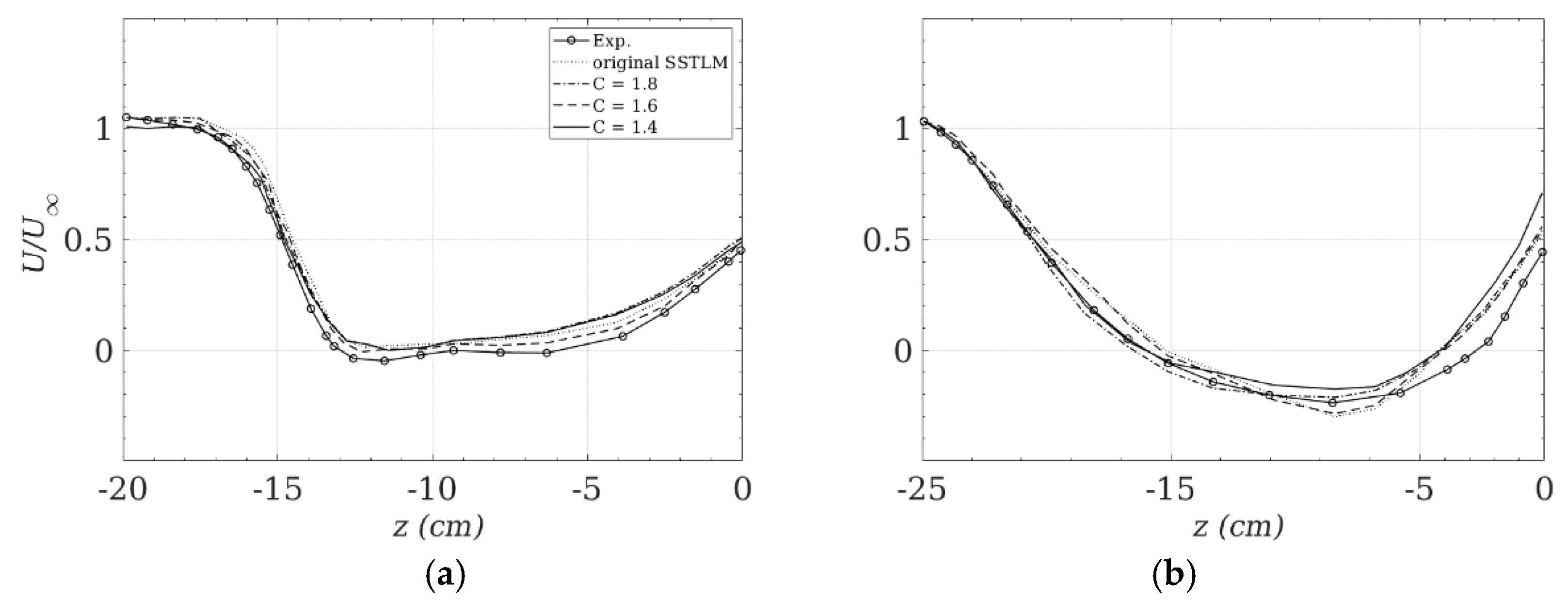
Figure 2 compares the results of the original and the tuned SSTLM model with experimental velocity measurements in the wake of upper arm and the extended leg. The measurement for the arm is at y = 1.1 m, and for the thigh is at y = 0.95 m. Both are extracted x/d = 0.8 downstream of the cross-section center, where d is the width of the cross-section. The root mean square errors between the predictions and experimental data are 1.1%, 0.5%, 1.1% and 0.9% for C = 1.4, 1.6, 1.8 and 2.193 (original), respectively, for the arm (Figure 2a), and 1.9%, 1.3%, 1.4% and 1.5% for the thigh (Figure 2b). A value of C = 1.6 shows the best agreement for both appendages, with the most significant improvement for the flow around the upper arm. For the remainder of the manuscript, C = 1.6 will be employed as the ‘Tuned SSTLM’ model. Table 1 shows that, with tuning, the estimate of C_dA improves from 7.8% error to 6.0%.

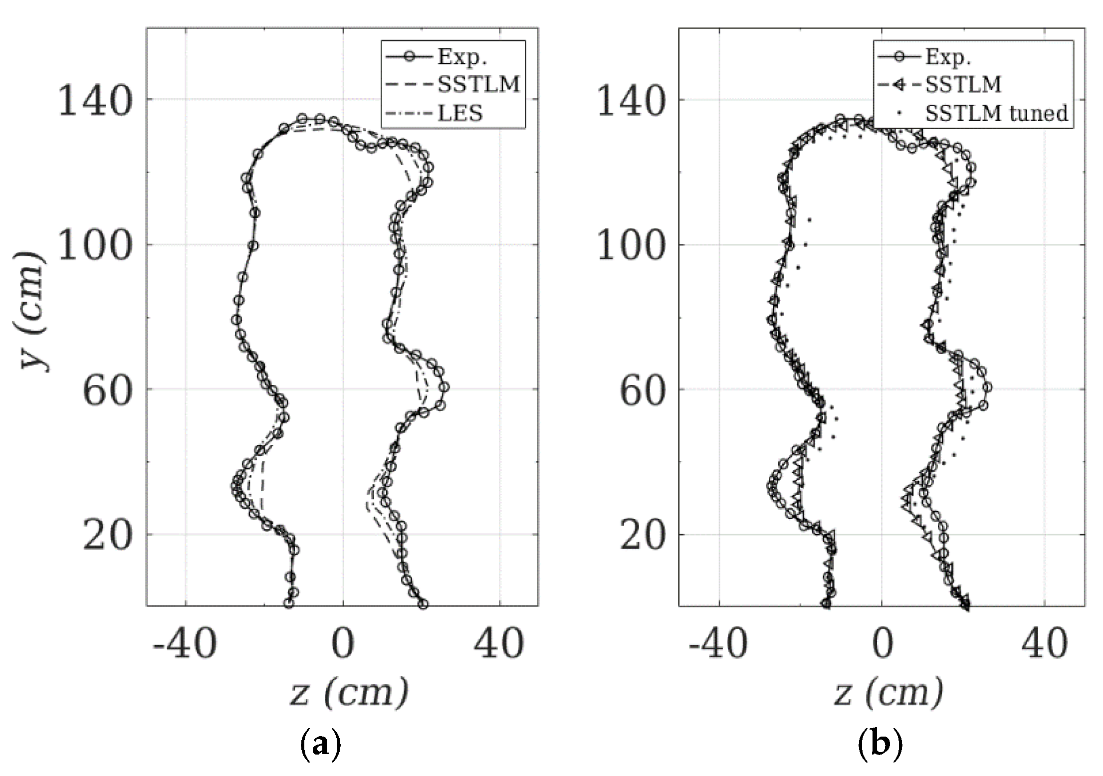
Figure 3 compares the contour of 0.90U_∞ for the different turbulence modeling approaches, using TLM in a yz-plane 0.8 m behind the rear wheel, with the experimental data of Terra et al. [8]. In general, the wake width is reasonably captured for both the LES and URANS methods, though URANS predicts the separation over the hip further downstream than does LES. The tuned SSTLM improves the prediction of the separation on the raised leg side of the hip (positive z); see Figure 2b. Stagnation regions with their strong pressure gradients, three-dimensional flow transition after stagnation, and separation over the hip are challenging to predict. LES predicts the torso wake well (z > 100), while it under-predicts the coherent structures generated from the feet (z ~ 40 and 60 for the left and right foot, respectively).

Overall, URANS with SSTLM predicts the large scale wake structures well; see Figure 3a. The intermittency equation in SSTLM needs very fine resolution close to the wall, with a zero normal flux boundary condition. It is only sensitive to streamwise velocity over the surface. The tuned model increases the intermittency, which increases the production of turbulent kinetic energy further upstream. The SST k−ω model limits the eddy viscosity to improve the performance of the model for adverse pressure gradients and in the wake regions. Nevertheless, SSTLM, which was developed for attached transitional flows, predicts a slightly more diffusive wake compared with the LES results; see Figure 3a.

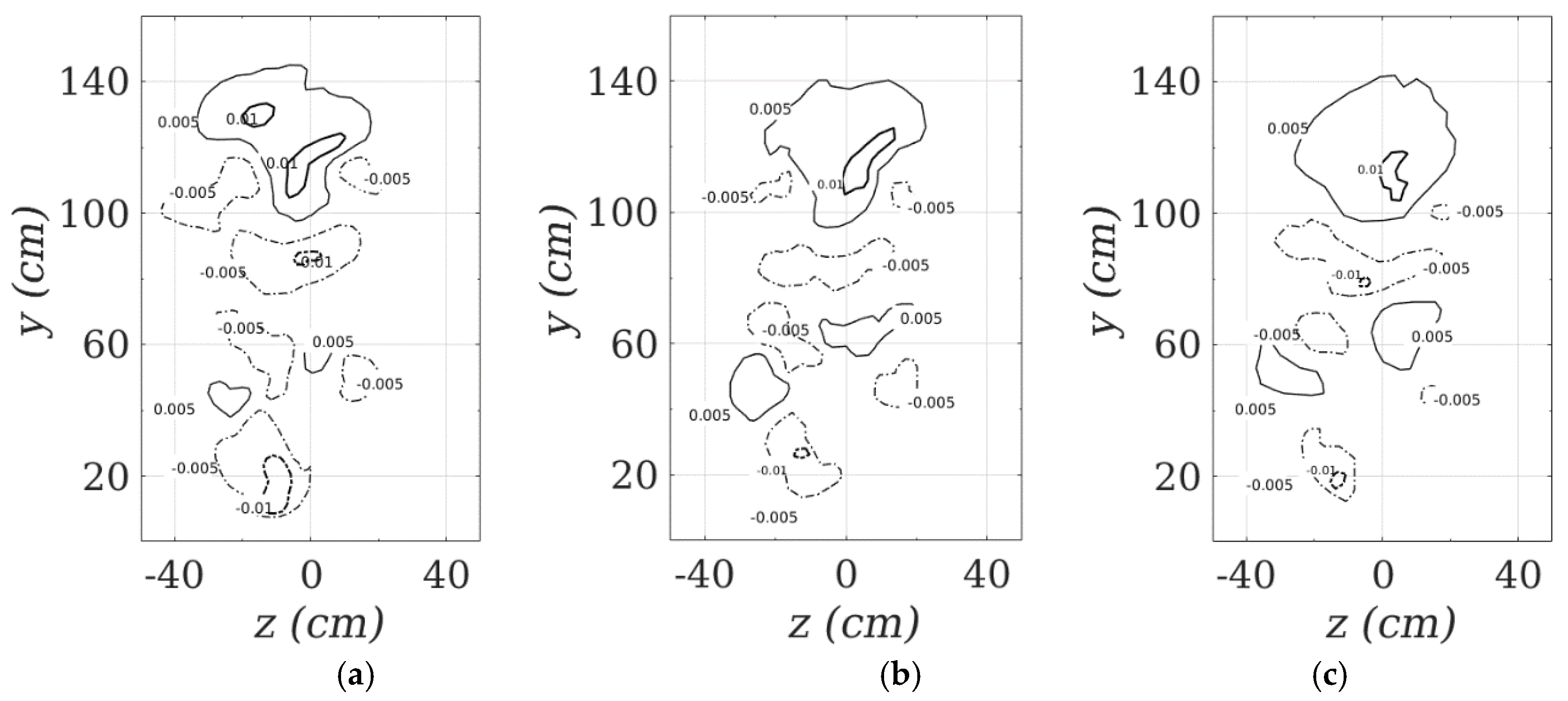
Figure 4 shows the pressure coefficient, C_p = (p-p_∞)/0.5ρU_∞², in the same plane as Figure 3 for the experimental and simulation data. Figure 4a shows that there is a high pressure region in 100 < z < 140, which is downstream of the rider’s torso. This pressure rise corresponds to the Bernoulli effect associated with the decrease in mean velocity in the wake of the cyclist. It also shows three low pressure regions in 80 < z < 100. These regions correspond with three main coherent structures in the wake of the cyclist. The strongest one, which is on the z-axis, is generated from the hip; the left one (negative z) is generated from the outer part of extended leg; and the right one (positive z) is generated from the outer part of raised leg. The low pressure region on the extended leg side is spatially larger than that of the raised leg. There are three other low pressure regions in z < 60, two of which are due to the coherent structures generated by the feet, and the remaining one is from the knee of the extended leg. The pressure coefficients from LES and SSTLM correspond well with the experimental measurements, with LES showing the best agreement; see Figure 4b. The low pressure regions predicted by SSTLM are smaller than those of the experimental measurement (see Figure 4c, indicating that SSTLM predicts smaller coherent structures than LES.

4. Conclusions

The flow around a cyclist was studied using two methods, URANS and LES, and two near wall treatments: two-layer wall modeling and Spalding’s law. The SSTLM turbulence model was used for the URANS simulations, as the flow was expected to be transitional around portions of the body. LES better predicts the drag area when using two-layer wall modelling, while Spalding’s law performs better for URANS. The LES drag area estimation is within 3.6% of the measured value, albeit at higher computational expense than URANS. URANS with SSTLM under-predicts the drag area by 7.8%. Examining the transition location around the appendages predicted by LES and SSTLM revealed that LES predicts transition further upstream. To rectify this, the SSTLM model was tuned, which resulted in an improvement in drag area estimation of 23%, in comparison with the original model, at no additional computational expense. Further revision of the SSTLM turbulence model, perhaps with the local values of the correlation coefficient, may provide additional improvements.