The Neural Network Zoo ^†

Abstract

An overview of neural network architectures is presented. Some of these architectures have been created in recent years, whereas others originate from many decades ago. Apart from providing a practical tool for comparing deep learning models, the Neural Network Zoo also uncovers a taxonomy of network architectures, their chronology, and traces back lineages and inspirations for these neural information processing systems.

1. Introduction

The past decade has witnessed a spectacular rise of interest in artificial intelligence, driven by large volumes of data being available for machine learning, decreasing costs for data storage and graphics processing units, and a technical and commercial infrastructure that allows for the commodification of intelligent applications. Deep learning, a particular branch of artificial intelligence that involves machine learning using multi-layered neural network models, is generally considered a key technology for the recent success in artificial intelligence. In order to gain insight into the interdependencies between these neural network models, and to support the discovery of new types, we decided to create a taxonomy of neural networks, uncovering some of the inspirations and underlying lineages of network architectures. This effort has resulted in the Neural Network Zoo, shown in Figure 1. For each of the models depicted, we wrote a brief description that includes a reference to the original publication.

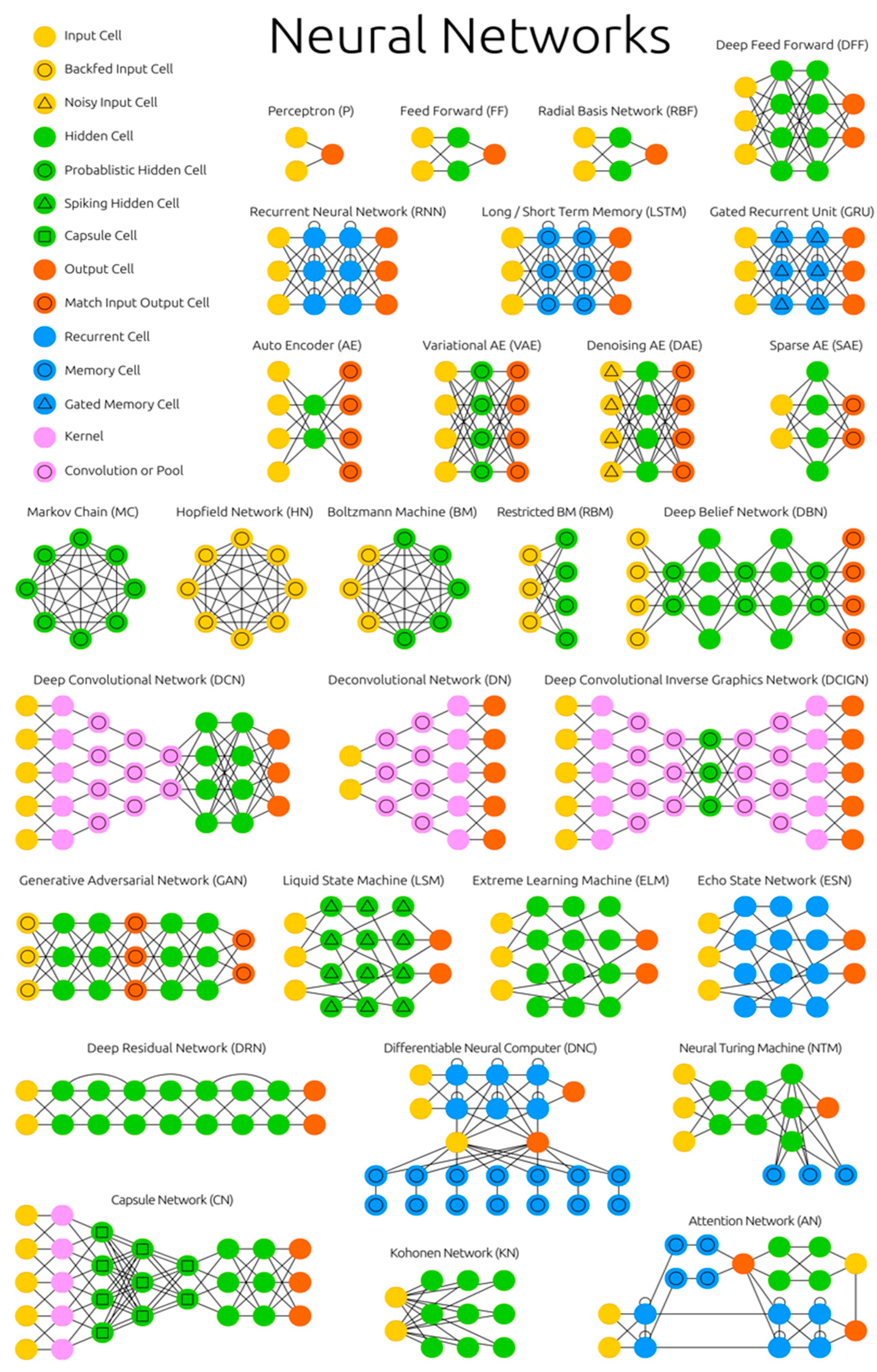
2. Neural Network Architectures

2.1. Feed Forward Neural Networks

Feedforward neural networks, including perceptrons [1] and radial basis function networks [2], transform patterns from input to output. They are the archetypical neural network, having layers that consist of either input, hidden or output nodes. Nodes are connected between adjacent layers, which can be fully connected (every neuron from one layer to every neuron in another layer). The minimal network has two input cells and one output cell that can be used to model logic gates, for example. Backpropagation is a common learning algorithm where the network is shown pairs input and expected output, and the strength of the connections between nodes is updated based on the model’s success in predicting. Theoretically, given infinite neurons in a single, nonlinear hidden layer, any relation between input and output patterns can be learned. However, having multiple hidden layers (thereby creating a deep network) can, in practice, lead to a more efficient learning process.

2.2. Recurrent Neural Networks

Recurrent networks are feedforward networks with connections within layers. Therefore, they are not stateless and the timing and order in which input is structured matters. This allows recurrent networks to find structure in time [4]. They can also be used with data modalities that are time-independent, such as images, by representing those as a sequence (e.g., of pixels). Training these networks may yield vanishing (or exploding) gradients, where, depending on the activation functions used, information gets lost (or amplified) over time, similar to how very deep feedforward networks can lose information in depth.

2.3. Long Short-Term Memory

LSTMs [5] provide a resolution for the vanishing and exploding gradient problems, by introducing gates and explicitly defined memory cells. Each node has a memory cell and three gates: Input, output, and forget. The function of these gates is to protect the loss of information by stopping or allowing it to flow. The input gate determines how much of the information from the previous layer is stored in the cell. The output gate determines what the next layer gets to know about the state of this cell. The forget gate prevents new information from being ignored. Gated recurrent units [6] are LSTMs with a different set of gates, making them faster but less expressive.

2.4. Autoencoders

Autoencoders [7] compress (encode) and regenerate (decode) information by transforming it through a smaller hidden layer with symmetrical surrounding layers. The resemblance between input and output can be used as a measure of success for the compression. Variational autoencoders [8] share a similar architecture, but instead, learn an approximate probability distribution of the input patterns grounded in Bayesian inference and modeling causal relations. Denoising autoencoders [9] are yet another type of autoencoder, where the input data are processed through a random noise filter (e.g., making an image grainy). The output is still compared to the original input image, so the network learns to ignore some of the detailed features that are not causally relevant. Finally, sparse autoencoders [10] do much of the inverse as they project information to a larger, rather than smaller, hidden layer. This allows the network to focus on smaller features in compressing and reconstructing the input data. To prevent information from being copied perfectly between layers, a filter is used for the error that is being backpropagated.

2.5. Hopfield Networks and Boltzmann Machines

In Hopfield networks [11], each neuron is connected to all other neurons, and all neurons are both input and output nodes. (Restricted) Boltzmann machines [12,13] are similar to the extent that only some neurons are input neurons, while others are hidden. Restricted Boltzmann machines do not have full connectivity between neurons, making them typically more efficient to be used for learning, particularly when they are stacked on top of each other in a so-called deep belief network [14]. Hopfield Networks and Boltzmann machines are trained by clamping the value of the input neurons to the desired pattern, after which the weights are learned. Once trained, the network will converge to one of the learned patterns and stay stable in one of these attractor states, in part due to the total energy in the network being reduced incrementally during training, similar to the Ising model. These network types are also called associative memories because they converge to the most similar state compared to their input. Markov Chains [15], though not neural network architectures themselves, are also included in this overview as they can be considered as predecessors.

2.6. Convolutional Networks

Convolutional networks [16] are deep learning architectures that typically contain convolutional and pooling layers, used for approximate scanning of patterns that are often spatially correlated. As such, they are useful for image processing, but they can be applied to other data modalities as well. Deconvolutional layers [17] produce the inverse results and can, therefore, be used for image generation. Deep convolutional inverse graphics networks [18] are yet another type that can be used to (partially) generate images, being similar to variational autoencoders but equipped with convolutional nodes for the encoding and decoding layers.

2.7. Generative Adversarial Networks

Generative adversarial networks [19] or GANs actually consist of two networks, one tasked with generating data (the generator), the other with predicting whether the data have been generated or not (the discriminator). The predictive success of the discriminator is used as an error gradient for the generator. This setup aims for the discriminator to get better at distinguishing real data from generated data, while the generator learns to become less predictable. This dynamical interplay can be viewed as a kind of Turing test, or a neural correlate of the Minimax algorithm. The learning process is relatively difficult to balance since it will not converge when either the generator or the discriminator is too successful at its respective task.

2.8. Liquid State Machines and Echo State Machines

Liquid State Machines [20] are not organized into neat layers, but rather, connections are randomly drawn between neurons with threshold functions that allow for the accumulation of activity over time, creating spiking activity patterns. Consequently, instead of using backpropagation, the input neurons are activated and the activity signals are propagated forward through the hidden neurons. The resulting propagation of signals itself is used for learning by a separate observer network that produces the output. Echo State Machines [21] replace these spiking neurons with the regular sigmoid activation neurons. Extreme Learning Machines [22] are similar but do not have recurrent connections, allowing them to be trained fast using a learning algorithm based on least-squares fit.

2.9. Deep Residual Networks

Another example of a network architecture that lacks structured layers are deep residual networks [23], feedforward networks where connections can pass any number of hidden layers. This makes them similar to recurrent neural networks but without the time preserving structure.

2.10. Neural Turing Machines and Differentiable Neural Computers

Neural Turing Machines [24] can be understood as an abstraction of LSTMs, and an attempt to make neural networks more explainable. Instead of coding a memory cell into a neuron, the memory is separated as a content-addressable memory where the neural network can write to and read from, making them Turing complete. Differentiable Neural Computers [25] are a further abstraction, with scalable memories. They also feature three attention mechanisms that allow the network to query the similarity of input to the memory entries, the temporal relationship between two memory entries, and whether a memory entry was recently updated.

2.11. Attention Networks

Attention networks [26] represent a class of networks rather than a particular architecture. They employ an attention mechanism to prevent information from vanishing by separately storing previous network states and switching attention between the states. This context can be visualized, providing interesting insights into the correlations between input features and predictions.

2.12. Kohonen Networks

Kohonen networks [27], or self-organizing maps, utilize competitive learning to classify input data without knowing the expected output, using an aesthetic objective function for successful classification. After presenting an input pattern, the network assesses which of its nodes most closely matches this input, and then adjusts them together with their neighboring nodes to further improve the matching.

2.13. Capsule Networks

Capsule networks [28] provide a biologically plausible alternative to pooling layers. Neurons are connected with a weight vector rather than a scalar value. This allows neurons to simultaneously transfer multiple types of information, e.g., not only which feature is detected but also where it is detected in a picture and what is its color and orientation. The learning algorithms are also biologically inspired by Hebbian learning that places value on accurate predictions of output in the next layer.

3. Conclusions

Considered chronologically, the network architectures presented in this paper generally grow in complexity, both in terms of numbers of layers and in types of neurons involved. We speculate that this trend is caused by the field of neural information processing systems becoming increasingly embraced by the engineering community, leading to a continued emphasis on practical applicability over biological inspiration and plausibility. Time will tell if this trend is here to stay.

This overview of neural networks aims to provide a list of the most popular methods used in deep learning, yet is far from complete. Moreover, new models will emerge. As they do, we will welcome these strange beasts into the Neural Network Zoo.

References

1. Rosenblatt, F. The perceptron: A probabilistic model for information storage and organization in the brain. Psychol. Rev. 1958, 65, 386. [Google Scholar] [CrossRef] [PubMed]
2. Broomhead, D.S.; Lowe, D. Radial Basis Functions, Multi-Variable Functional Interpolation and Adaptive Networks; RSE-MEMO-4148; Royal Signals and Radar Establishment Malvern: Farnborough, UK, 1988. [Google Scholar]
3. The Neural Network Zoo. Available online: http://www.asimovinstitute.org/neural-network-zoo (accessed on 10 April 2020).
4. Elman, J.L. Finding structure in time. Cogn. Sci. 1990, 14, 179–211. [Google Scholar] [CrossRef]
5. Hochreiter, S.; Schmidhuber, J. Long short-term memory. Neural Comput. 1997, 9, 1735–1780. [Google Scholar] [CrossRef] [PubMed]
6. Chung, J.; Gulcehre, C.; Cho, K.; Bengio, Y. Empirical evaluation of gated recurrent neural networks on sequence modeling. arXiv 2014, arXiv:1412.3555. [Google Scholar]
7. Bourlard, H.; Kamp, Y. Auto-association by multilayer perceptrons and singular value decomposition. Biol. Cybern. 1988, 59, 291–294. [Google Scholar] [CrossRef]
8. Kingma, D.P.; Welling, M. Auto-encoding variational bayes. arXiv 2013, arXiv:1312.6114. [Google Scholar]
9. Vincent, P.; Larochelle, H.; Bengio, Y.; Manzagol, P.A. Extracting and composing robust features with denoising autoencoders. In Proceedings of the 25th International Conference of Machine Learning, Helsinki, Finland, 5–9 July 2008. [Google Scholar]
10. Ranzato, M.A.; Poultney, C.; Chopra, S.; Cun, Y.L. Efficient learning of sparse representations with an energy-based model. In Proceedings of the NIPS, Vancouver, BC, Canada, 3–6 December 2007. [Google Scholar]
11. Hopfield, J.J. Neural Networks and physical systems with emergent collective computational abilities. Proc. Natl. Acad. Sci. USA 1982, 79, 2554–2558. [Google Scholar] [CrossRef]
12. Hinton, G.E.; Sejnowski, T.J. Learning and relearning in Boltzmann machines. Parallel Distrib. Process. Explor. Microstruct. Cogn. 1986, 1, 282–317. [Google Scholar]
13. Smolensky, P. Information Processing in Dynamical Systems: Foundations of Harmony Theory; No. CU-CS-321-86; Colorado Univ at Boulder Dept of Computer Science: Boulder, CO, USA, 1986. [Google Scholar]
14. Bengio, Y.; Lamblin, P.; Popovici, D.; Larochelle, H. Greedy layer-wise training of deep networks. Adv. Neural Inf. Process. Syst. 2007, 19, 153. [Google Scholar]
15. Hayes, B. First links in the Markov chain. Am. Sci. 2013, 101, 252. [Google Scholar] [CrossRef]
16. LeCun, Y.; Bottou, L.; Bengio, Y.; Haffner, P. Gradient-based learning applied to document recognition. Proc. IEEE 1998, 86, 2278–2324. [Google Scholar] [CrossRef]
17. Zeiler, M.D.; Krishnan, D.; Taylor, G.W.; Fergus, R. Deconvolutional networks. In Proceedings of the 2010 IEEE Computer Society Conference on Computer Vision and Pattern Recognition, San Francisco, CA, USA, 13–15 June 2010. [Google Scholar]
18. Kulkarni, T.D.; Whitney, W.F.; Kohli, P.; Tenenbaum, J. Deep convolutional inverse graphics network. In Proceedings of the Advances in Neural Information Processing Systems, Montreal, QC, Canada, 7–12 December 2015. [Google Scholar]
19. Goodfellow, I.; Pouget-Abadie, J.; Mirza, M.; Xu, B.; Warde-Farley, D.; Ozair, S.; Courville, A.; Bengio, Y. Generative adversarial nets. In Proceedings of the Advances in Neural Information Processing Systems, Montreal, QC, Canada, 7–12 December 2014. [Google Scholar]
20. Maas, W.; Natschläger, T.; Markram, H. Real-time computing without stable states: A new framework for neural computation based on pertubations. Neural Comput. 2002, 14, 2531–2560. [Google Scholar] [CrossRef] [PubMed]
21. Jaeger, H.; Haas, H. Harnessing nonlinearity: Predicting chaotic systems and saving energy in wireless communication. Science 2004, 304, 78–80. [Google Scholar] [CrossRef] [PubMed]
22. Huang, G.B.; Zhu, Q.Y.; Siew, C.K. Extreme learning machine: Theory and applications. Neurocomputing 2006, 70, 489–501. [Google Scholar] [CrossRef]
23. He, K.; Zhang, X.; Ren, S.; Sun, J. Deep residual learning for image recognition. arXiv 2015, arXiv:1512.03385. [Google Scholar]
24. Graves, A.; Wayne, G.; Danihelke, I. Neuralturing machines. arXiv 2014, arXiv:1410.5401. [Google Scholar]
25. Graves, A.; Wayne, G.; Reynolds, M.; Harley, T.; Danihelka, I.; Grabska-Barwińska, A.; Colmenarejo, S.G.; Grefenstette, E.; Ramalho, T.; Agapiou, J. Hybrid computing using a neural network with dynamic external memory. Nature 2016, 538, 471–476. [Google Scholar] [CrossRef]
26. Jaderberg, M.; Simonyan, K.; Zisserman, A. SpatialTransformer Network. In Proceedings of the Advances in Neural Information Processing Systems, Montreal, QC, Canada, 7–12 December 2015; pp. 2017–2025. [Google Scholar]
27. Kohonen, T. Self-organized formation of topologically correct feature maps. Biol. Cybern. 1982, 43, 59–69. [Google Scholar] [CrossRef]
28. Sabour, S.; Frosst, N.; Hinton, G.E. Dynamic Routing Between Capsules. In Proceedings of the Advances in Neural Information Processing Systems, Long Beach, CA, USA, 4–9 December 2017; pp. 3856–3866. [Google Scholar]
Figure 1. An overview of neural network architectures [3].
Proceedings 47 00009 g001
Publisher’s Note: MDPI stays neutral with regard to jurisdictional claims in published maps and institutional affiliations.