Graph Entropy Associated with Multilevel Atomic Excitation ^†

Abstract

A graph-model is presented to describe multilevel atomic structure. As an example, we take the double $\mathsf{\Lambda }$ configuration in alkali-metal atoms with hyperfine structure and nuclear spin $I=3/2$, as a graph with four vertices. Links are treated as coherence. We introduce the transition matrix which describes the connectivity matrix in static graph-model. In general, the transition matrix describes spatiotemporal behavior of the dynamic graph-model. Furthermore, it describes multiple connections and self-looping of vertices. The atomic excitation is made by short pulses, in order that the hyperfine structure is well resolved. Entropy associated with the proposed dynamic graph-model is used to identify transitions as well as local stabilization in the system without invoking the energy concept of the propagated pulses.

1. Introduction

Propagation of optical pulses in gaseous media have been extensively discussed in terms of self-induced-transparency (SIT) [1,2] as well as electromagnetically-induced-transparency (EIT) [3]. SIT for two-level systems interpreted soliton formation through energy conservation. This simple picture is complicated for multilevel atoms. The condition for stabilization in energy and area of the pulses becomes no longer valid [4]. This is due to multiple light storage effects in the course of propagation [5]. In this paper, we aim to provide an alternative technique to study local stabilization in terms of entropy. The importance of our technique is that it interprets transitions between locally stable periods in space in terms of transitions between space-entropy thresholds. In addition, we present the multilevel structure in alkali atom as a graph. We are motivated by image processing and entropy [6], as well as quantum recurrent neural networks [7]. The graph-model consists of nodes and links as well as self-looping. The limitations of our proposed technique are fairly discussed.

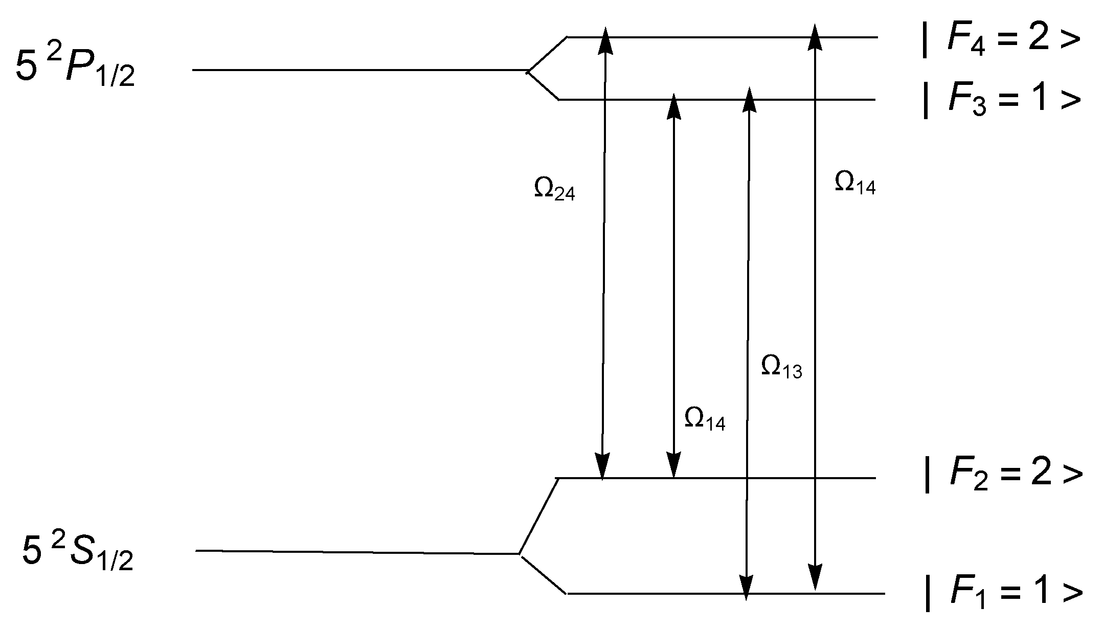
2. Theoretical Description

This paper presents quadrupole coherent excitation of ${}^{87}Rb$ vapor taking into account hyperfine structure of the $D_1$ line, i.e., $5{}^2{S}_{1/2}-5{}^2{P}_{1/2}$. The lower hyperfine (hf) levels are presented as $|1\rangle =|5{}^2{S}_{1/2},F=1\rangle$, and $|2\rangle =|5{}^2{S}_{1/2},F=2\rangle$, while the upper hf levels are described by $|3\rangle =|5{}^2{P}_{1/2},F=1\rangle$ and $|4\rangle =|5{}^2{P}_{1/2},F=2\rangle$, where F denotes the total angular momentum quantum number. These four bare states form the standard configuration for double V or double $\mathsf{\Lambda }$ electromagnetically induced transparency (EIT). The Maxwell fields connect the dipole allowed transitions. The fields with Rabi frequencies ${\mathsf{\Omega }}_{13}$ and ${\mathsf{\Omega }}_{14}$ connect the optical transitions $1\leftrightarrow 3$ and $1\leftrightarrow 4$, respectively. In addition, the fields with Rabi frequencies ${\mathsf{\Omega }}_{23}$, and ${\mathsf{\Omega }}_{24}$ connect the optical transitions $2\leftrightarrow 3$ and $2\leftrightarrow 4$, respectively. Figure 1 shows the energy level diagram for the $D_1$ line including hyperfine structure associated with the coupling fields.

The state of the dressed atom is described by Liouville–von Neumann type equation for the reduced density matrix [4,8]. Let $(z,t)$ represent space-time coordinates in the laboratory frame. c is the light speed. The dimensionless retarded time in a frame moving with pulse is denoted by $\tau =\gamma (t-z/c)$, where $\gamma$ is the spontaneous decay rate of the excited atomic state $P_{1/2}$. The dimensionless space variable is given as $\zeta ={\alpha }^{{}^{\prime }}(z+ct)$ and ${\alpha }^{{}^{\prime }}$ is the absorption coefficient of one of the pulses at $z=0$. The atom field coupling v is defined as $v=\frac{dE}{2\sqrt{3}}$, where d is the dipole moment of the optical transition and E is the electric field amplitude. The Rabi frequency is related to atom field coupling by the relation: $\mathsf{\Omega }=\sqrt{8}v$. The relative atom field coupling becomes: $\mathrm{v}=v/\gamma$. As far as the density matrix is concerned, we have 28 density matrix components (dmc) ${\rho }_{\alpha \beta }^{\left(Fm\right)}$ associated with the $D_1$ line taking into account the hf structure. $\alpha$ and $\beta$ take values from 1 to 4, F is the tensor rank representing the total angular momentum, and m is the magnetic quantum number. There are four components with zero rank ${\rho }_{\alpha \alpha }^{\left(00\right)}$ representing the populations of the hyperfine levels which satisfy the normalization condition $\sqrt{3}{\rho }_{11}^{\left(00\right)}+\sqrt{5}{\rho }_{22}^{\left(00\right)}+\sqrt{3}{\rho }_{33}^{\left(00\right)}+\sqrt{5}{\rho }_{44}^{\left(00\right)}=1$. Together with eight components with rank one representing the optical coherence such as ${\rho }_{\alpha \beta }^{\left(1m\right)}$, with $\alpha \ne \beta$. In addition, there are eight components with quadrupole-order. These are the Raman coherence ${\rho }_{43}^{\left(2m\right)}$, ${\rho }_{21}^{\left(2m\right)}$ for upper and lower hf levels, respectively. There are four components for the alignment of hf levels such as ${\rho }_{\alpha \alpha }^{\left(2m\right)}$, $\alpha =1,...,4$. The correlations between upper and lower hf levels are described by six matrix elements of octupole-order, such as ${\rho }_{\alpha \beta }^{\left(3m\right)}$ with $\alpha \ne \beta$. Finally, we have two components with hexadecapole-order as ${\rho }_{\alpha \alpha }^{\left(4m\right)}$ and $\alpha =2$ and 4. In this paper, we assume that the excitation is made by short pulses of time duration $T_p$ such that $\gamma T_p=0.1$. This ensures that the hf splitting is resolved. The time evolution of the dmc is presented in [4]. In the slowly varying approximation, the reduced-Maxwell field equations can be written as:

$$\begin{array}{c}\partial {\mathrm{v}}_{13}(\zeta ,\tau )/\partial \zeta =-{\rho }_{13}^{\left(10\right)}(\zeta ,\tau ),\partial {\mathrm{v}}_{23}(\zeta ,\tau )/\partial \zeta ={\rho }_{14}^{\left(10\right)}(\zeta ,\tau ),\hfill \\ \partial {\mathrm{v}}_{14}(\zeta ,\tau )/\partial \zeta =-{\rho }_{23}^{\left(10\right)}(\zeta ,\tau ),\partial {\mathrm{v}}_{24}(\zeta ,\tau )/\partial \zeta ={\rho }_{24}^{\left(10\right)}(\zeta ,\tau ).\hfill \end{array}$$

(1)

Initially, we assume that all atoms are at the first hyperfine level, i.e. $n_1(z=0,t=0)=\sqrt{3}{\rho }_{11}^{\left(00\right)}=1$. The radiation fields at entrance point $z=0$ are pulsed in the form $t^2$ Gaussian as $v\left(t\right)=64\sqrt{2\pi }/27v_0{(t/T_p)}^{2}exp(-8/9\pi {(t/T_p)}^2)$. The parameter $v_0$ represents the mean pulse amplitude. These pulses have the same mean field amplitude and the same duration. Finally, we have chosen that initially all the excitation pulses have the same area ${\theta }_0=7.8\pi$. The pulses are resonant to their respective dipole-allowed transitions in order to have a well defined area [9].

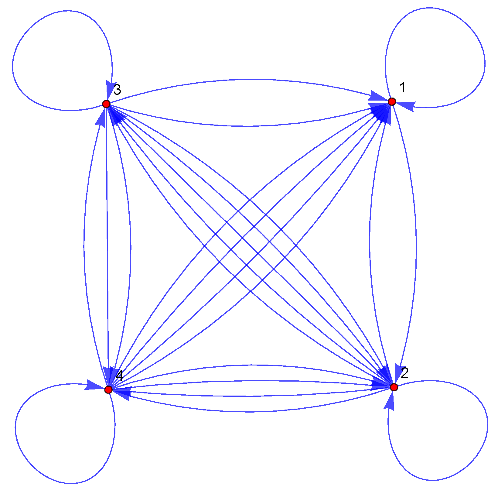
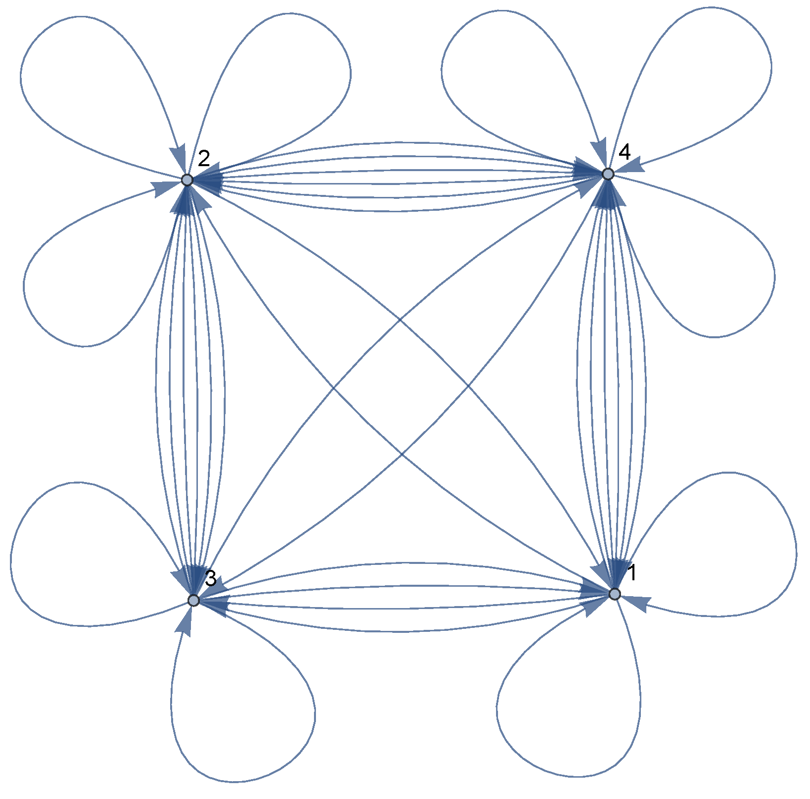
3. Graph Description

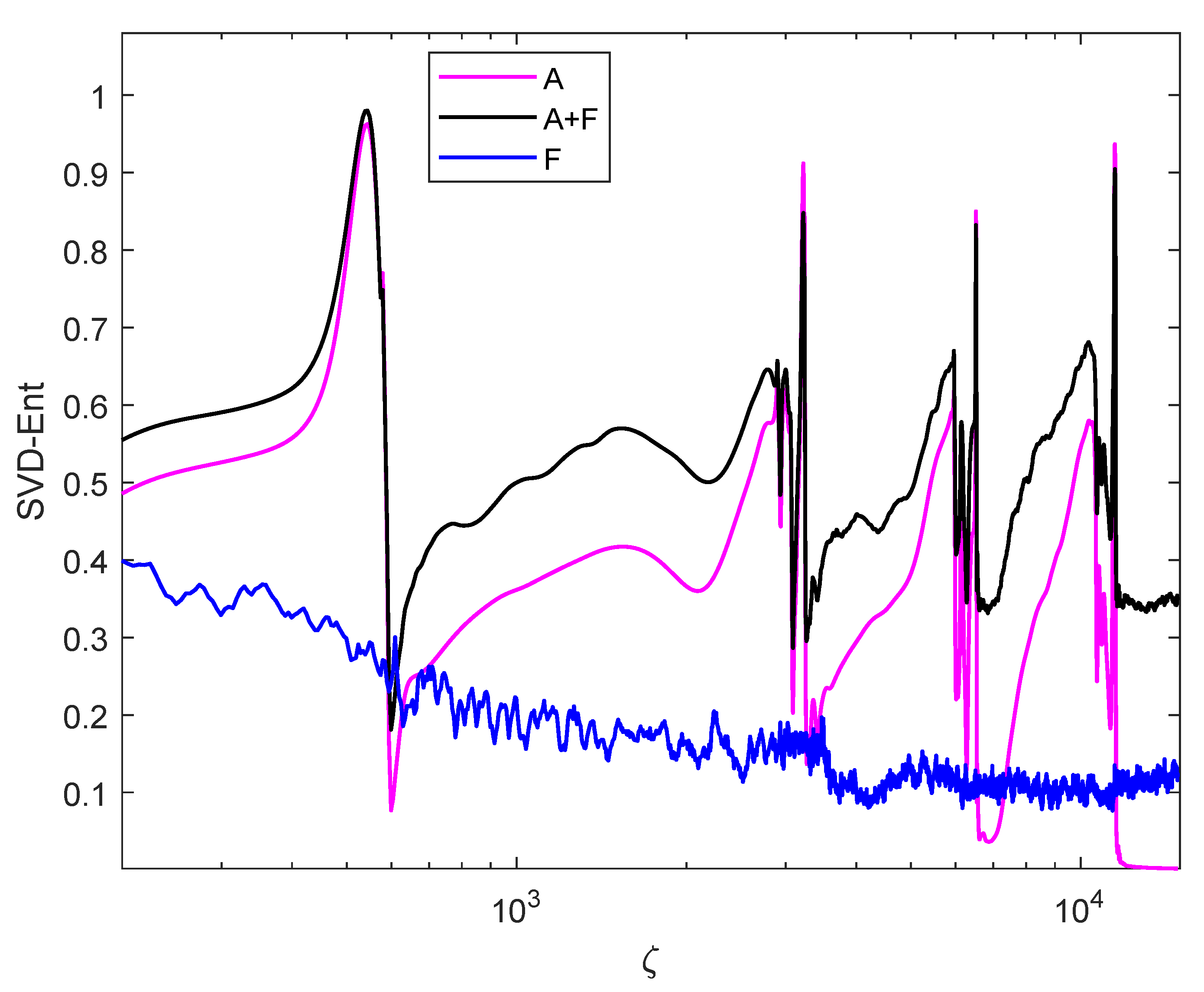
Let us present a graph-model which corresponds to hf structure, as illustrated in Figure 1. To do so, we have to introduce the connectivity matrix describing such multilevel structure. We use the term transition matrix instead of connectivity matrix to indicate that connections are dynamic implying time dependence as well as space dependence. The transition matrix $M(t;z)$ represents atomic as well as field contributions. We write its argument in terms of $(t;z)$. The semicolon indicates that we first solve Liouville–von Neumann equation in time at fixed space point [4]. In the next step, we solve the reduced-Maxwell field equations in space at fixed times. Rabi frequencies ${\mathsf{\Omega }}_{\alpha \beta }$ where $\alpha \ne \beta$ facilitate the field links in the graph-model. The atomic contributions to the transition matrix are written in the form ${\rho }_{\alpha \beta }^{\left(Fm\right)}$ and $\alpha \ne \beta$. The rank F satisfies the relation $\mid F_{\alpha }-F_{\beta }\mid \le \mathrm{F}\le F_{\alpha }+F_{\beta }$.

To begin with, we consider the case when links on the graph are represented by dmc of first and second rank tensors.

The graph for double $\mathsf{\Lambda }$ configuration consists of four vertices. The vertices of lower hf levels are labeled as $\left|1\right.〉\rangle =|F_1=1\rangle \langle F_1=1|\mathrm{and}\left|2\right.〉\rangle =|F_2=2\rangle \langle F_2=2|$, while the vertices of the upper hf levels are denoted by: $\left|3\right.〉\rangle =|F_3=1\rangle \langle F_3=1|$ and $\left|4\right.〉\rangle =|F_4=2\rangle \langle F_4=2|$. The transition matrix connects vertices through coherence of the first rank ${\rho }_{\alpha \beta ;\alpha \ne \beta }^{\left(10\right)}$ as well as the Raman tensors ${\rho }_{12}^{\left(20\right)}$ and ${\rho }_{34}^{\left(20\right)}$, which are tensors of the second rank. Furthermore, the atom-field couplings $v_{\alpha \beta ;\alpha \ne \beta }$ are also considered as links between vertices. Self-looping is represented by atomic populations ${\rho }_{\alpha \alpha }^{\left(00\right)}$ and $\alpha =1,2,3,\mathrm{and}4$. The resulting transition matrix as a graph-model corresponding to hf structure illustrated in Figure 1 is represented by:

$$M_1(t;z)=\left(\begin{array}{ccccccc}{\rho }_{11}^{\left(00\right)}& {\rho }_{11}^{\left(20\right)}& {\rho }_{12}^{\left(2m\right)}& {\rho }_{23}^{\left(1m\right)}& {\rho }_{34}^{\left(2m\right)}& {\rho }_{41}^{\left(1m\right)}& v_{41}\\ {\rho }_{21}^{\left(2m\right)}& {\rho }_{12}^{\left(20\right)}& {\rho }_{22}^{\left(00\right)}& {\rho }_{23}^{\left(1m\right)}& v_{23}& {\rho }_{34}^{\left(2m\right)}& v_{42}\\ {\rho }_{31}^{\left(1m\right)}& v_{31}& {\rho }_{32}^{\left(1m\right)}& v_{32}& {\rho }_{33}^{\left(00\right)}& {\rho }_{34}^{\left(2m\right)}& {\rho }_{43}^{\left(2m\right)}\\ {\rho }_{41}^{\left(1m\right)}& v_{41}& {\rho }_{12}^{\left(2m\right)}& {\rho }_{23}^{\left(1m\right)}& v_{23}& {\rho }_{34}^{\left(2m\right)}& {\rho }_{44}^{\left(00\right)}\end{array}\right)$$

(2)

This description contains fields as well as tensors of first and second ranks. Figure 2 shows the graph-model based upon the transition matrix $M_1(t;z)$.

Let us consider a sub matrix from the matrix $M_1(t;z)$ that contains the connections as the atomic coherence and self-looping as:

$$M_2(t;z)=\left(\begin{array}{ccccc}{\rho }_{11}^{\left(00\right)}& {\rho }_{12}^{\left(2m\right)}& {\rho }_{23}^{\left(1m\right)}& {\rho }_{34}^{\left(2m\right)}& {\rho }_{41}^{\left(1m\right)}\\ {\rho }_{21}^{\left(2m\right)}& {\rho }_{22}^{\left(00\right)}& {\rho }_{23}^{\left(1m\right)}& {\rho }_{34}^{\left(2m\right)}& {\rho }_{42}^{\left(1m\right)}\\ {\rho }_{31}^{\left(1m\right)}& {\rho }_{12}^{\left(2m\right)}& {\rho }_{23}^{\left(10\right)}& {\rho }_{34}^{\left(2m\right)}& {\rho }_{43}^{\left(2m\right)}\\ {\rho }_{41}^{\left(1m\right)}& {\rho }_{21}^{\left(2m\right)}& {\rho }_{13}^{\left(1m\right)}& {\rho }_{34}^{\left(20\right)}& {\rho }_{44}^{\left(40\right)}\end{array}\right)$$

(3)

We can define another matrix for the field connections only as:

$$M_3(t;z)=\left(\begin{array}{cc}{v}_{13}\left(t\right)& v_{32}\left(t\right)\\ v_{24}\left(t\right)& v_{41}\left(t\right)\end{array}\right)$$

(4)

Let us write the transition matrix as composed from the coherence.

$$M_4(t;z)=\left(\begin{array}{cccc}{\rho }_{12}^{\left(2m\right)}& {\rho }_{23}^{\left(1m\right)}& {\rho }_{34}^{\left(2m\right)}& {\rho }_{14}^{\left(1m\right)}\\ {\rho }_{12}^{\left(2m\right)}& {\rho }_{13}^{\left(1m\right)}& {\rho }_{34}^{\left(2m\right)}& {\rho }_{24}^{\left(1m\right)}\\ {\rho }_{13}^{\left(1m\right)}& {\rho }_{12}^{\left(2m\right)}& {\rho }_{24}^{\left(1m\right)}& {\rho }_{23}^{\left(1m\right)}\\ {\rho }_{14}^{\left(1m\right)}& {\rho }_{12}^{\left(2m\right)}& {\rho }_{23}^{\left(1m\right)}& {\rho }_{34}^{\left(2m\right)}\end{array}\right)$$

(5)

We write atomic contributions to the transition matrix in terms of the density matrix components from the zeroth rank to the fourth rank as:

$$M_5(t;z)=\left(\begin{array}{ccccccc}{\rho }_{11}^{\left(00\right)}& {\rho }_{13}^{\left(1m\right)}& {\rho }_{23}^{\left(1m\right)}& {\rho }_{12}^{\left(2m\right)}& {\rho }_{11}^{\left(20\right)}& {\rho }_{24}^{\left(3m\right)}& {\rho }_{14}^{\left(3m\right)}\\ {\rho }_{22}^{\left(00\right)}& {\rho }_{31}^{\left(1m\right)}& {\rho }_{32}^{\left(1m\right)}& {\rho }_{21}^{\left(2m\right)}& {\rho }_{22}^{\left(20\right)}& {\rho }_{42}^{\left(3m\right)}& {\rho }_{41}^{\left(3m\right)}\\ {\rho }_{33}^{\left(00\right)}& {\rho }_{14}^{\left(1m\right)}& {\rho }_{24}^{\left(1m\right)}& {\rho }_{34}^{\left(2m\right)}& {\rho }_{33}^{\left(20\right)}& {\rho }_{23}^{\left(3m\right)}& {\rho }_{22}^{\left(40\right)}\\ {\rho }_{44}^{\left(00\right)}& {\rho }_{14}^{\left(1m\right)}& {\rho }_{42}^{\left(1m\right)}& {\rho }_{43}^{\left(2m\right)}& {\rho }_{44}^{\left(20\right)}& {\rho }_{32}^{\left(3m\right)}& {\rho }_{44}^{\left(40\right)}\end{array}\right)$$

(6)

We take the magnetic quantum number $m=0$ for linearly polarized light propagation. Furthermore, we consider the full transition matrix as composed from the atomic as well as the field contributions as

$$M_6(t;z)=M_6^a(t;z)+M_6^b(t;z),$$

(7)

where

$$M_6^a(t;z)=\left(\begin{array}{ccccccc}{\rho }_{11}^{\left(00\right)}& {\rho }_{13}^{\left(1m\right)}& {\rho }_{14}^{\left(1m\right)}& {\rho }_{23}^{\left(1m\right)}& {\rho }_{24}^{\left(1m\right)}& {\rho }_{11}^{\left(20\right)}& {\rho }_{12}^{\left(2m\right)}\\ {\rho }_{22}^{\left(00\right)}& v_{13}& v_{14}& v_{23}& v_{24}& {\rho }_{22}^{\left(20\right)}& {\rho }_{21}^{\left(2m\right)}\\ {\rho }_{33}^{\left(00\right)}& {\rho }_{31}^{\left(1m\right)}& {\rho }_{41}^{\left(1m\right)}& {\rho }_{32}^{\left(1m\right)}& {\rho }_{42}^{\left(1m\right)}& {\rho }_{33}^{\left(20\right)}& {\rho }_{34}^{\left(2m\right)}\\ {\rho }_{44}^{\left(00\right)}& v_{31}& v_{41}& v_{32}& v_{42}& {\rho }_{44}^{\left(20\right)}& {\rho }_{43}^{\left(2m\right)}\end{array}\right)$$

(8)

and

$$M_6^b(t;z)=\left(\begin{array}{cc}{\rho }_{24}^{\left(3m\right)}& {\rho }_{14}^{\left(3m\right)}\\ {\rho }_{42}^{\left(3m\right)}& {\rho }_{41}^{\left(3m\right)}\\ {\rho }_{23}^{\left(3m\right)}& {\rho }_{22}^{\left(40\right)}\\ {\rho }_{32}^{\left(3m\right)}& {\rho }_{44}^{\left(40\right)}\end{array}\right)$$

(9)

Figure 3 presents the network associated with the transition matrix $M_6(t;z)$. It contains a full description of the atomic dmc as well as the components of the radiation field transitions. The nodes are labeled from 1 to 4. Nodes 1 and 3 are associated with two components of self-looping, the population of the hf levels, and the second rank tensors describing the alignment of hf levels. Nodes 2 and 4 are associated with three components of self-looping, the population of the hf levels, and the second rank tensors describing the alignment of hf levels, as well as the hexadecapole components with forth rank tensors. The diagonals in the figure represent Raman coherence, which describes tensor alignment with second-order tensors. The off-diagonal links represent coherence of the first- and third-order tensors as well as the transition fields.

4. Graph-Entropy

In this section, we provide mathematical formalism for graph-entropy. We introduce the transition matrix $M(t;z)$ associated with a model graph representing the hf structure. There are different views of $M(t;z)$ depending upon the ranks of density matrix included to construct the links and vertices. The graph-entropy which we aim to introduce is not for static configuration. However, it is dynamic, in the sense that the transition matrix depends implicitly on time. The state of the transition matrix is determined by time evolution governed by linear Liouville–von Neumann-type equation for the density matrix. Moreover, the transition matrix depends implicitly on time and space as well. This dependence is governed by space-time evolution of reduced Maxwell’s field equations. Some of transition matrices are square and others are triangular. Therefore, we prefer to calculate eigenvalues through the Singular Value Decomposition (SVD) technique, even though the matrix is a square matrix. The positiveness of eigenvalues simplify our formalism for obtaining probabilities.

In the following, we aim to describe the procedure to obtain graph-entropy. Let us note that our transition matrix is not in general symmetric. Thus, $M_{\alpha \beta }\ne M_{\beta \alpha }$. This symmetry absence due to our arrangement of dmc in $M(t;z)$ rows and columns. The sequence of density matrix elements in every arrangement is not unique. We present some transition matrices. It is to be noted that $M_1(t;z)$ contains coherence tensors of the first and second rank as well as dipole fields as links between graph vertices. We also have tensors of the second rank representing tensor alignments. Figure 2 presents a graph -model based upon the transition matrix $M_1(t;z)$. The transition matrix $M_2(t;z)$ contains coherence tensors and tensors of the fourth rank. The transition matrix $M_3(t;z)$ contains only fields as links, while the transition matrix $M_4(t;z)$ contains dmc of the first rank and third rank coherence.

Thus far, we have constructed different representatives for the transition matrix. We attempt to compare entropy obtained from: (a) the matrix $M_6(t;z)$, which contains full description of the atomic as well as the field components; (b) the matrix $M_5(t;z)$, which contains the atomic components only; and (c) the matrix $M_3(t;z)$, which describes the radiation fields. The eigenvalues are obtained at space-time points through propagation of the pulses. Let us calculate the eigenvalues $\lambda (t;z)$ for each transition matrix. Then, we define the probability function over eigenvalues as:

$$P_M\left(\lambda (t;z)\right)=\frac{\lambda (t;z)}{{\sum }_{\lambda }\lambda (t;z)}$$

(10)

Space-time dependent von Neumann entropy for each class of transition matrices can be written as

$$H_M(t;z)=-\sum _{\lambda }{P}_M\left(\lambda (t;z)\right){log}_2{P}_M\left(\lambda (t;z)\right).$$

(11)

Finally, we integrate space-time-dependent von Neumann entropy over time to obtain residual von Neumann entropy as:

$$S_M\left(z\right)={\int }_T{H}_M(t;z)dt.$$

(12)

where T denotes the range of times. The finial time used is taken as $\gamma t=10$.

One may aware about the number of configurations associated with the transition matrix $M(t;z)$ in order to have a valid or right way of connections between nodes of the graph. As an example, nodes 1 and 2 are only connected by second rank coherence tensors, not with other rank tensors. In fact, we do not take into account the influence of permutation entropy on our constrained transition matrix $M(t;z)$. However, differences due different arrangement of $M(t;z)$ elements are presented. We show in Figure 4 SVD-entropy as the residual von Neumann entropy for different classes of the transition matrix $M(t;z)$. By residual, we mean integrated over time. The black line represents SVD-entropy for full matrix of information about the system depicted in Figure 1. It contains the atomic as well as the field contributions. The magenta line represents SVD-entropy associated with the atomic contributions only, while the blue line represents the field contribution. The SVD-entropy for the case A+F shows that it is greater than SVD-entropy for atoms only. Both SVD-entropy lines show multiple transitions in the course of propagation. These transitions are due to interference effects between eigenvalues. For big distances, the atomic contribution to SVD-entropy diminishes, where the field contribution lasts longer. Therefore, SVD-entropy for A+F remains finite at big distances. Figure 5 presents the results when we do some rearrangement of elements in $M_6(t;z)$ matrix, where we move the field components to the last two columns in Equation (Section 3). The difference in SVD-entropy for the two transition matrix is small for big distances where the atomic contribution to entropy is small. Thus, we conclude that SVD-entropy is not unique and depends on the arrangement chosen to represent the transition matrix. However, in this case, we attempt mainly to reveal the system’s behavior showing the locations of non-linearity that are exposed by peaks downwards or upwards. In fact, these transition are due to interference effects among different ranks of the density matrix [8]. Figure 4 and Figure 5 show the spikes with maximum-entropy and minimum-entropy. We compare the behavior of space-dependent entropy in Figure 4 and Figure 5 with the space-dependent behavior for the area of the pulses and its energies obtained in [9]. The initial areas are the same in both cases with the same shapes as well as pulse durations. Unfortunately, our program takes around one month to produce new results for comparison. In comparison, we observe that, within these spikes of Figure 4 and Figure 5, one can find area stabilization. In addition, maximum-entropy and minimum-entropy signify pulse area transitions nearby from $2n\pi$ to nearby $2(n-1)\pi$, where n, here, is an integer, $n=4,3,2$ and 1.

5. Conclusions

The goal of our paper is to detect by entropy means other formations of radiation transitions without appealing to SIT or EIT concepts. We show that space-dependent von Neumann entropy, through SVD spectrum of eigenvalues, reveals space-dependent transitions for entropy due to different classes of transition matrices. We compare the space behavior of our previous results on area development and energy attenuation with those presented here, for space-entropy [9]. We conclude that space-entropy points out the area transitions from nearby $2n\pi$ to nearby $(2n-1)\pi$ for the field $v_{14}\left(t\right)$. In addition, space-entropy points out the abrupt changes in energy. We use the word “nearly” because the area theorem does not hold beyond the two-level atom approximation. In conclusion, we introduce a graph-model for the excitation of multilevel atoms. The proposed technique describes transition matrix representing connections in dynamic graph-model. The space-time dependence of von Neumann entropy is obtained. Residual entropy is defined as integral of von Neumann entropy over time. We show that residual entropy exposes transitions in the course of propagation. These transitions are devoted to interference effects among eigenvalues. Maximum as well as minimum entropy signify critical upper and lower bounds for pulse stabilization, respectively. In between these limits, the entropy increases towards maximum entropy. The maximum entropy points out transitions from nearby $2n\pi$ to nearby $(2n-1)\pi$ in area, where n is an integer. Figure 4 and Figure 5 clearly expose four peaks. The positions of entropy transitions correspond to area transitions from $8\pi \to 6\pi \to 4\pi \to 2\pi$, and eventually to $0\pi$ value. One can associate the difference $\Delta S\left(z\right)$ to information content about the system at space points. Threshold entropy values are critical entropy. Beyond critical entropy, pulse breakup, and soliton formation may occur. We consider full basis to generate the Liouville difference space. This enables us to consider third- and forth-order dmc as links and self-looping in the graph-model, respectively. Our numerical results for third- and forth-order dmc show that it also points out radiation transitions. However, it is not presented due to the lack of space in the paper. It is to be noted that these components are rarely or not used in the literature of pulsed light propagation. Its importance lies on the fact that it results in small and new peaks that give fine structure to space-entropy. Low rank tensor description of residual entropy is, in our opinion, misleading.

References

1. McCall, S.L.; Hahn, F.L. Self-induced transparency by pulsed coherent light. Phys. Rev. Lett. 1967, 18. [Google Scholar] [CrossRef]
2. Slusher, R.E.; Gibbs, H.M. Self-Induced Transparency in Atomic Rubidium. Phys. Rev. A 1972, 5, 1634. [Google Scholar] [CrossRef]
3. Boller, K.J.; Imamoglu, A.; Harris, S.E. Observation of Electromagnetically Induced Transparency. Phys. Rev. Lett. 1991, 66, 2593–2596. [Google Scholar] [CrossRef] [PubMed]
4. Alhasan, A.M. Entropy Associated with Local Stabilization of the Pulse Area in Multilevel Atomic Media. Act. Phys. Pol. A 2018, 133, 5. [Google Scholar] [CrossRef]
5. Alhasan, A.M. Advanced soliton-train generation through drive field enhancement and multiple light storage effect in cold rubidium atoms. Eur. Phys. J. Spec. Top. 2007, 144, 277–282. [Google Scholar] [CrossRef]
6. Sparavigna, A.C. Entropy in Image Analysis. Entropy 2019, 21, 502. [Google Scholar] [CrossRef] [PubMed]
7. Gandi, V. Brain-Computer Interfacing for Assistive Robotics: Electroencephalograms, Recurrent Quantum Neural Networks, and User-Centric Graphical Interfaces; Academic Press, Elsevier Inc.: Amsterdam, The Netherlands, 2015. [Google Scholar] [CrossRef]
8. Alhasan, A.M. Entropy Associated with Information Storage and Its Retrieval. Entropy 2015, 17, 5920–5937. [Google Scholar] [CrossRef]
9. Alhasan, A.M. Short pulses propagation in multilevel atomic media. AIP Conf. Proc. 2018, 1976, 020005. [Google Scholar] [CrossRef]
Figure 1. Energy level diagram of the D 1 transition in 87 R b atom including hyperfine structure.
Proceedings 46 00009 g001
Figure 2. Graph-model based upon the transition matrix M 1 ( t ; z ) and corresponding to energy level diagram for the D 1 transition in 87 R b atom including hyperfine structure, as depicted in Figure 1.
Proceedings 46 00009 g002
Figure 3. Graph-model based upon the transition matrix M 6 ( t ; z ) , which includes full details of the atomic components of the density matrix as well as the transition field contributions.
Proceedings 46 00009 g003
Figure 4. Space-dependent SVD-entropy as the residual von Neumann entropy for different classes of the transition matrix M ( t ; z ) .
Proceedings 46 00009 g004
Figure 5. Space-dependent SVD-entropy as the residual von Neumann entropy for different classes of the transition matrix as M 6 ( t ; z ) and its modified version. We replace the atomic components in the last two columns of Equation (Section 3) by the field components.
Proceedings 46 00009 g005
Publisher’s Note: MDPI stays neutral with regard to jurisdictional claims in published maps and institutional affiliations.