Published: 14 November 2019
1. Introduction
Inertial Navigation System (INS) is a system that uses Inertial Measurements Unit (IMU) sensors to calculate the orientation, velocity and position of a platform using the combination of accelerometers and gyroscopes of the IMU. The typical low-cost IMU based on Micro-Electro-Mechanical-System (MEMS) technology contains 3-axis orthogonal gyroscopes and 3-axis orthogonal accelerometers on the same silicon die [
1].
IMUs are used in a variety of applications but in particular for navigation. Since the IMUs measurements are not accurate and have significant errors that causes the navigation solution to drift over time [
2]. That is why in most cases, in addition to the INS, a larger navigation system that contains additional external accurate measurements units (e.g., GPS or compass) is used. When there are some constrains that prevent the usage of external measurement (e.g., GPS in urban environments), the INS is the main unit in the navigation system calculation, leading to inaccuracy in the navigation solution.
One of the approaches to circumvent a rapid solution drift is to use a multi IMU (MIMU) architecture [
3]. The motivation to use of multiple low-cost IMUs is to improve performance of several navigation related issues in a scope of a simple low-cost solution. Theoretically, the usage of a large number of IMUs should enable the reduction of noise and by that reducing the system’s errors [
3,
4]. Another advantage of using a large number of IMUs, is the option to continue receiving data from the system even when one of the sensors malfunctions for some reason, which is impossible do to when using only one IMUs system.
As in the MIMU architecture, a gyro-free (GF) INS has multiple accelerometers, but no gyroscopes [
5]. A GFINS consists of at least six distributed accelerometers capable of obtaining linear and angular acceleration and thereby capable of functioning as a conventional INS. Most of the research in the gyro-free is focused on seeking optimal configurations [
6]. A practical GF kinematic equation of motion and corresponding error-state models, fitting any accelerometer configuration was derived [
7]. Recently, a state-of-the-art literature review of GFINS and a control theoretic point of view was provided in [
8].
In this research, a feasibility study of MIMU consisting of 32 IMUs was conducted. Different MIMU configurations were examined and the one with the smallest error metric was chosen for the further experiments. To that end, a software tool to parse the data and analyze them including IMU calibration, solving equations of motion and filtering abilities was derived. Additionally, a dedicated hardware architecture was designed. Using the MIMU software and hardware we focus on sensor calibration differences between a single IMU and a 32 based MIMU. Results show that the latter is preferred in terms of accuracy and time to converge.
This rest of the paper is organized as follows:
Section 2 discusses the theoretical background while
Section 3 presents the experiment structure–software and hardware.
Section 4 presents the experiments and the results of the research subjects of the MIMU system.
Section 5 gives the conclusions and the suggestions for further research.
2. Problem Formulation-Theoretical Background
A single IMU has 6 sensors, when each sensor has measurement errors. The major types of errors are bias error, white noise error and drift error. The bias error is a constant systematic error that is differ for each sensor. This type of error can be reduced by calibrating the data of each sensor. The second error, white noise error, is a random error. It is a statistical error with unknown size that is different for each sensor, and different for each sample. The third error, drift error, is an error that accumulates in the direction of the sensor movement [
4].
In theory, a system with a large amount of the same sensors (e.g., MIMU), has a smaller statistical error than a single sensor system. According to the Central limit theorem, when the number of sensors in the system is N, and N approaches infinity, the expected value of the error is 0 (a system without white noise).
In practice, when N is finite, the error’s size will be divided by
. Indeed, the standard deviation of the error will be divided by
. We can see it by the definition of the standard deviation:
where
is the random variables vector of the full system (with N IMUs components) in the sample
k.
is the random variables vector of IMU number
i in the system, in the sample
k. We assume that
equals to
, it means that the random variables are independent and identically distributed (IID).
is the standard deviations vector in the sample
k, and
N is the number of IMU components in the MIMU system. It is important to note that the variables are vectored (length of 6), when each component in the vector represents a different sensor in the IMU.
The linear acceleration
a is defined as in [
1]:
where
f is the acceleration vector (with three coordinates) measured by the IMU’s sensors and
g is the local gravity acceleration vector.
The position, velocity and Euler’s angles of the platform can be calculated according to Equations (3)–(5), assuming that the earth turn rate can be neglected:
where
p is the position in meters and
v is the velocity,
is a 3 × 3 transformation matrix between the body and navigation frames,
is the specific force vector and g is the gravity. The addition vector
in (5) is based on (2).
is the angular velocity vector expressed in its skew-symmetric
where
is the angular velocity around i axis. Solving (3)–(5) gives the navigation solution for low-cost sensors.
By using the transform matrix for time t, we can calculate Euler’s angles [
2]:
3. Hardware and Software Tools
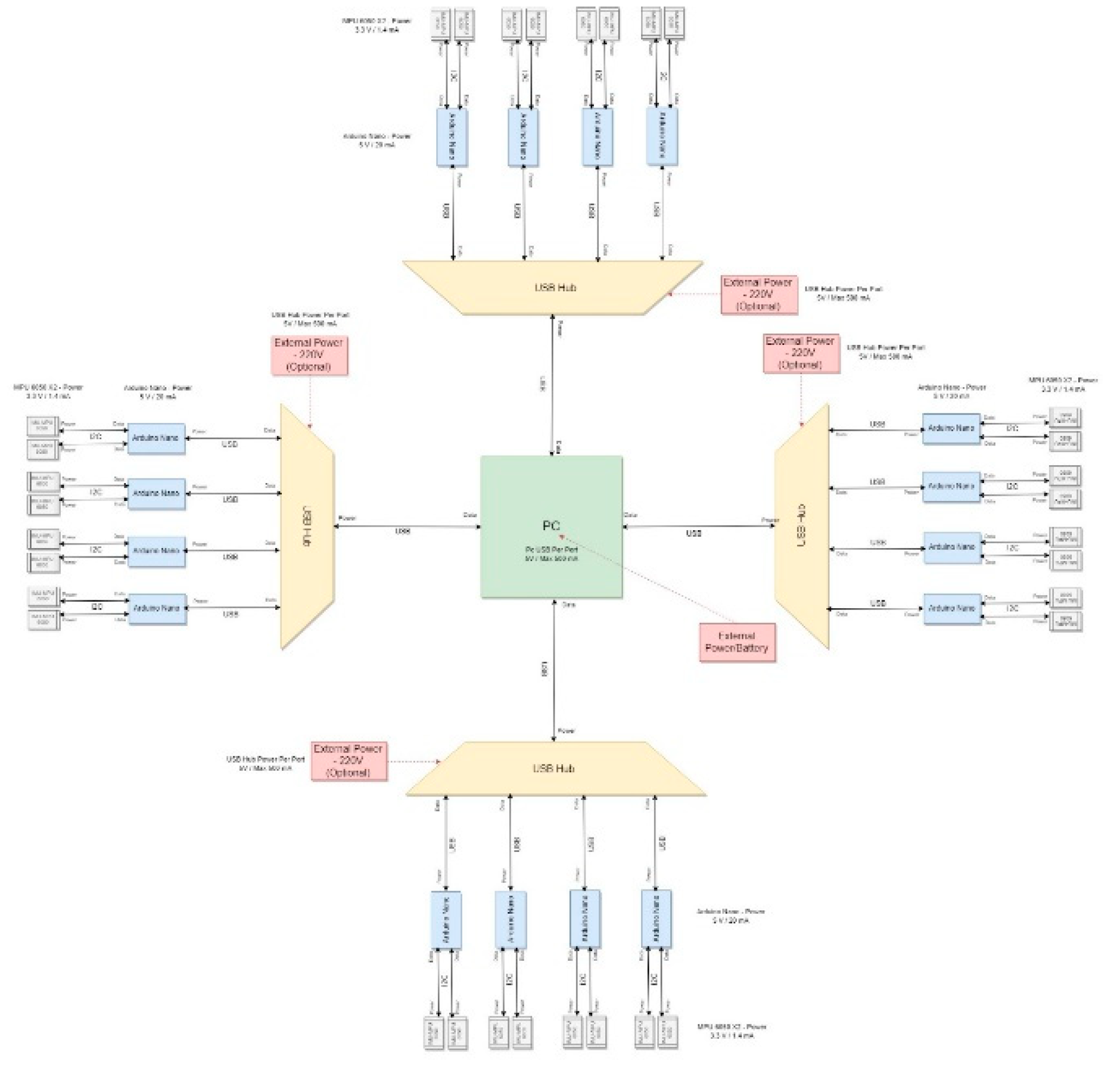
The MIMU system that was built for the research was based on MPU-6050 IMU. Every two MPU6050 sensors were connected to one Arduino Nano controller by the I2C protocol. The Arduino redirects the results from the IMUs to a PC (accelerometers and gyroscopes data), at a rate sample of 100 Hz. The MIMU system contained 32 IMU components controlled by 16 Arduino controllers. 32 IMU components were chosen due to hardware and cost considerations. Each IMU’s price was about 1
$ therefore the 32 IMU components price was about 32
$. The system can be easily expanded thanks to its modularity. The MIMU system scheme is illustrated in
Figure 1:
The Arduino controller program code was implemented to receive the MIMU components data. Those sensor results were exported to a CSV file that included the measurements of the accelerometers and gyroscopes. Afterwards we used a dedicated tool to analyze the data and receive position, velocity and Euler’s angles of the MIMU system. The main functions of the tool are:
Alignment of the samples—usually the begging and the end of the sampling time are different between the Arduinos in the MIMU system. Therefore, the tool cuts the edges of the data so that all sensor results will be at the same timing.
Calibration of the samples—for each metric of each IMU component, the tool calculates the average of the sampling results from the beginning until a specific time (calibration time), when the system is at rest. Afterwards, for each metric, the tool subtracts the calculated average value from the metric results.
Main SW tool—a dedicated tool to analyze the data of all IMUs and averaging their results. This tool uses Low Pass filter as part of the analyze implemented with FFT algorithm. Moreover, the tool also uses Tuckey’s Fences algorithm to remove outliers. Finally, the tool averages all the components result to one MIMU’s system results.
Solving equations of motion–the SW tool also solves the equations of motion according to the formulas listed in the theoretical
Section 2. For the given input, which contains angular velocity and linear acceleration, the tool calculates the linear velocity and the position of the system all in the navigation axis system using transition matrix. Furthermore, Euler angles are also calculated using the transition matrix.
4. Experiments and Results
The experiment made were focused on examining the effect of MIMU system on the calibration performance. After finding the optimal configurations (e.g., filter configurations), the systems sensors were measured for 5 min. This experiment was repeated 3 times in stationary conditions (3 different sets of measurements).
First, we examined the position errors of each system. As mentioned in
Section 3, during the process we solved the equations of motion. The IMU measurements were plugged in (3)–(5) to calculate the position. Since the system was stationary, Euler’s angles, velocity and position are fixed. We used those solutions as the baseline that corresponds to lack of calibration. Afterwards we also calculated the position with calibrated sensors by solving again the equations of motion. During the calibration, we calculated each sensor’s average value for a period of time. The average value approached the bias error which was removed as part of the process. In the
Table 1, we can see the results for the 32 components MIMU system and 1 IMU system positions, with calibration for 10 s and without calibration (baseline):
Our main research question: for stationary platform MIMU system containing 32 IMU components with allowable calibration time of 10 s, how much time is needed to calibrate 1 IMU system, and receive the same position error as the MIMU system?
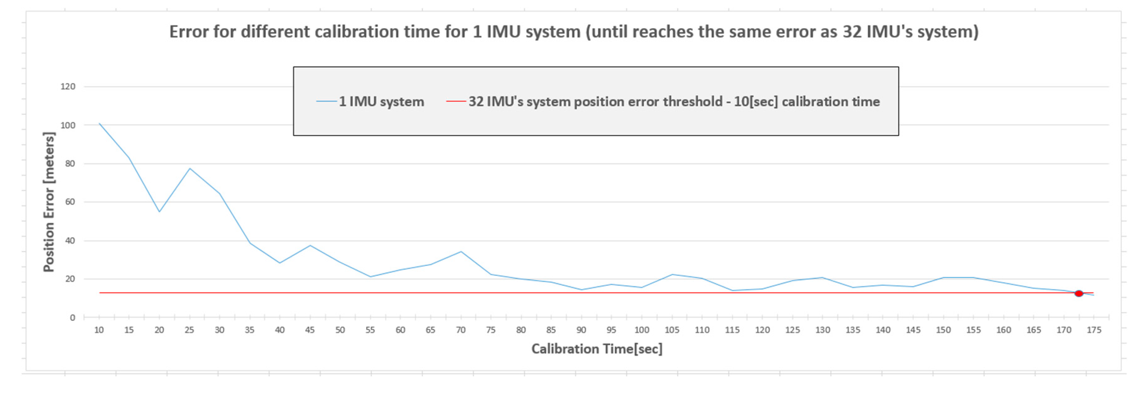
Next, the 32 components MIMU system position error was measured during 10 s of calibration. Afterward, 1 IMU system was examined in iterations. In each iteration 5 s were added to the calibration time, until the 1 IMU system had the same position error as the 32 components MIMU system. The results depending on calibration time are presented in
Figure 2:
We can see that there is a trend of reduce in the position error as the calibration time of the 1 IMU system is increasing. However, the error reduction is not monotonous. Furthermore, the position error of the 1 IMU system is smaller than the 32 components MIMU system, only after 175 s of calibration. (when the 32 components MIMU’s system calibration time is 10 s).
5. Discussion and Conclusions
In this paper, a 32 based MIMU architecture was designed and used for field experiments. Those were focused on the benefit of using MIMU for calibration of inertial sensors. Results show that a single IMU system requires about 175 s of calibration to obtain the same performance as the 32 based MIMU system that was calibrated for 10 s. This result show that a MIMU obtains better performance using the same calibration time. In addition, the time to reach the same performance was reduced by a factor of 17. We could also see that the MIMU’s system errors are smaller than the 1 IMU’s system errors. Indeed, the position error was divided by the factor of 8.11 when using the MIMU system. Theoretically, the errors were expected to be divided by (1).
To achieve a better view on the MIMU’s system advantages we are continuing our research with more experiments that will answer more questions. (1) Should the order of solving the equations of motion be before or after the averaging and filtering process? (2) What is the influence of the different IMUs locations on the MIMU system platform configurations? (3) What is the influence of the number of components on the MIMU’s system errors?


