Acoustic Bragg Peak Localization in Proton Therapy Treatment: Simulation Studies ^†

Abstract

A full chain simulation of the acoustic hadron therapy monitoring for brain tumors is presented in this work. For the study, a proton beam of 100 MeV was considered. In the first stage, Geant4 was used to simulate the energy deposition and to study the behavior of the Bragg peak. The energy deposition in the medium produced local heating that can be considered instantaneous with respect to the hydrodynamic time scale producing a sound pressure wave. The resulting thermoacoustic signal was subsequently obtained by solving the thermoacoustic equation. The acoustic propagation was simulated by the Finite Element Method (FEM) in the brain and the skull, where a set of piezoelectric sensors were placed. Lastly, the final received signals in the sensors were processed in order to reconstruct the position of the thermal source and, thus, to determine the feasibility and accuracy of acoustic beam monitoring in hadron therapy.

1. Introduction

The use of heavy particles as protons in the treatment against solid tumors in areas not accessible with standard photon radiation has been increasing in recent decades [1]. This is shown in the number of new accelerators in new centers of proton therapy [2]. The main advantage of protons over photons is the dose distribution, minimizing the damage to tissue out of the region near the Bragg peak region. The location of the Bragg peak profile depends mainly on the initial energy of the beam and its width. This deposition is particularly important in clinical conditions with a total energy deposit, such as melanoma of the eye or tumors in brain tissue, among others, where the possibility of damage to nearby tissue increases due to the size of the tumor tissue. Although monitoring and control systems are carried out before and after each radiation session, different alternatives for the monitoring process have been proposed based on physical processes produced in the irradiated medium such as prompt-gammas, charged particles, $\mathsf{\beta }\mathsf{þ}$-emitter, and PET-imaging [3]. This article proposes an alternative method based on the pressure produced by the proton beam, the amplitude of which was evaluated from a set of piezoelectric sensors. In particular, it is based on simulated studies of the absorbed dose distribution for a set of energies from the Monte Carlo methods. Thus, the thermoacoustic model calculates the pressure received at a point in space that will be one of the input parameters for the Finite Element Method (FEM) that solves the behavior of the piezoelectric effect in a piezoelectric (PZT) material as the set of sensors for brain tumor applications.

2. Monte Carlo Simulation

In order to calculate the energy deposited in the water due to the Bragg peak, the Monte Carlo methods were applied using the Geant4 hadron therapy simulation package. The model features a 100 MeV monoenergetic proton beam using the Electromagnetic Quark–Gluon String model with Binary Cascade for primary protons (QGSP BIC EMY) as Physics List [4]. The absorbent material was G4Water with a density of 1003 $\mathrm{kg}/{\mathrm{m}}^3$ and a number of simulations of about ${10}^6$ histories. The detector volume consisted of a solid G4Box with a voxel size of 1 mm. To evaluate the boundary conditions of bone tissue, the Anthropomorphic model was used within the Geant4 libraries. The models were simulated in the volume of water including the bone structure. Generally, in medical physics applications, the results of Geant4 are evaluated in dose deposit per unit area, however, in this study, the energy of the beam deposited in the tissue was evaluated. Thus, the behavior of the Bragg peak was used in its energy part in the thermoacoustic model described in the following section.

3. Thermoacoustic Model

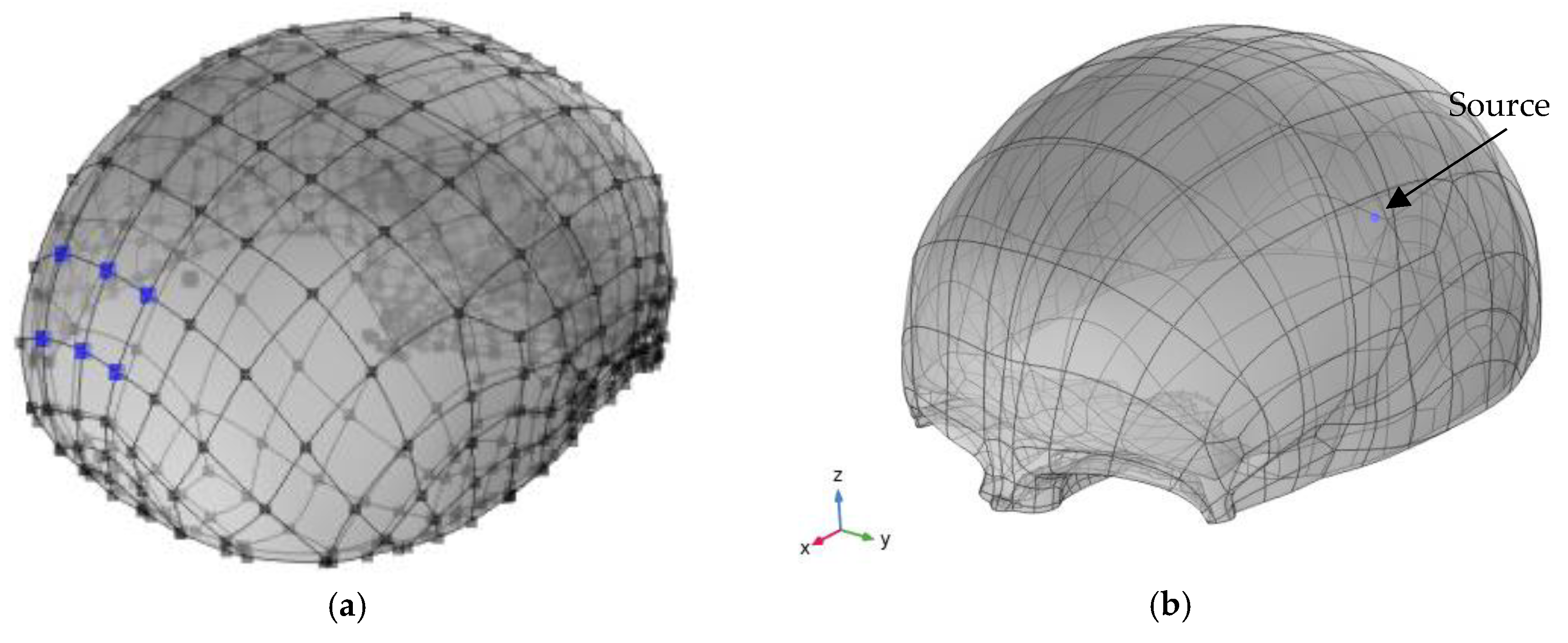
According to the Thermoacoustic model [5], the deposition of energy from particles that pass through a liquid produces local heating in the medium that can be considered instantaneous with respect to the hydrodynamic time scale. Due to the temperature change, the medium either expands or contracts according to its coefficient of volumetric expansion $\alpha$. The accelerated movement of the heated medium forms a pressure pulse that propagates through the fluid. The model is described in Equation (1), with the particular solution given in Equation (2).

$${\overline{\nabla }}^{2}p\left(\overrightarrow{r},t\right)=-\frac{1}{c_s^2}·\frac{{\partial }^{2}p\left(\overrightarrow{r},t\right)}{\partial t^2}=-\frac{\alpha }{C_p}·\frac{{\partial }^2ϵ\left(\overrightarrow{r},t\right)}{\partial t^2}$$

(1)

$$p\left(\overrightarrow{r},t\right)=\frac{1}{4\pi }\frac{\alpha }{C_p}{{\displaystyle \int }}_V^{}\frac{d{V}^{\prime }}{\left|\overrightarrow{r}-{\overrightarrow{r}}^{\prime }\right|}·\frac{{\partial }^2}{\partial t^2}ϵ\left({\overrightarrow{r}}^{\prime },t-\frac{\left|\overrightarrow{r}-{\overrightarrow{r}}^{\prime }\right|}{c_s}\right)$$

(2)

where $p(\overrightarrow{r},t)$ is the pressure at a snapshot in time $t$, and spatial position $\overrightarrow{r}$, $c_s$ represents the speed of sound in the middle; $C_p$ is the specific heat; $ϵ(\overrightarrow{r},t)$ is the energy density deposited in the medium; and $\alpha$ is the coefficient of thermal expansion. When a pulse of protons radiates in a homogeneous volume, it corresponds to a pressure source proportional to the energy deposition $ϵ(\overrightarrow{r},t)$. Each differential volume element of the irradiated source pressure emits a micro bipolar pressure wave. The pressure measured in the sensor is the sum of the micro-pressure waves emitted by each differential element of the volume. Due to the constant speed of sound throughout the medium, from the perspective of the sensor, the pressure that arrives after a certain time t is related to the pressure waves emitted in a common radius r. As shown in Equation (1), the derivative of these pressure waves translates a bipolar behavior that is eventually the signal received by the sensor.

4. FEM Simulation

To solve the problem of propagation of the pressure calculated at a certain distance from the Bragg peak, the FEM model was used for acoustic-structure iteration, which combined the Pressure Acoustics, Transient, and Solid Mechanics interfaces to connect the acoustics pressure variations in the fluid domain with structural deformation in the solid domain. In essence, the default sound pressure function models harmonic sound waves in the water domain using Equation (3) for sound pressure.

$$\frac{1}{{\rho }_0{c}_s^2}\frac{{ð}^{2}p}{ðt^2}+\nabla ·\left(-\frac{1}{\rho }\left(\nabla \mathrm{p}-q_d\right)\right)=Q_m$$

(3)

where $p$ is the pressure, and ${\rho }_0$ represents the density. $Q_m$ is the monopole domain source that corresponds to a mass source on the right-hand side of the continuity equation. The dipole domain source $q_d$ corresponds to a domain force source on the right-hand side of the momentum equation. The combination ${\rho }_0{c}_s^2$ is called the adiabatic bulk modulus, commonly denoted $Q_m$. The bulk modulus is equal to one over the adiabatic compressibility coefficient $\beta =1/K_s=1/{\rho }_0{c}_s^2$ [6]. The pressure generated by the thermoacoustic model is distributed in a sphere within the skull corresponding to the range of the Bragg peak deposition. Figure 1 shows the geometric model implemented in COMSOL Multiphysics and the positions of the sensors. The pressure value propagated to a spherical volume of 2 mm in diameter, which corresponded to the Bragg peak for 100 MeV, as shown in Figure 2b.

5. Localization Method

For the reconstruction of the position of the Bragg Peak, a system of nonlinear equations of the form $F\left(X\right)=0$, was solved using Newton’s method [7]. Consider a system of $m$ equations and $n$ unknowns:

$$f_m\left(x_1,x_2,x_3,\dots ,x_n\right)=0.$$

(4)

This system can be written in vector form as $f\left(x\right)=0$, where $f$ is a vector of $m$ dimensions, and $x$ is a vector of $n$ dimensions. To solve this system of equations, we have to find a vector $x$ such that the function $f\left(x\right)$ equals the null vector. If we call $\eta$ to the solution of the system and $x_r$ to an approximation of it, we can develop $f$ in Taylor series around this approximation as:

$$f\left(x\right)=f\left(x_r\right)+\nabla f\left(x_r\right)·\left(x-x_r\right)+\dots .$$

(5)

Since $f\left(\eta \right)=0$, then we get, as an approximation, the following:

$$0\approx f\left(x_r\right)+\nabla f\left(x_r\right)·\left(\eta -x_r\right),$$

(6)

defining the vector $x_{r+1}$ as this approximation, which is closer to the root than $x_r$. We can continue with the iterative method to obtain approximations closer and closer to the solution. To write the iterative method, the term $\nabla f\left(x_r\right)$ is replaced by the Jacobian of the function $f$, that is:

$$J\left(x_r\right)=\left[\begin{array}{cccc}\frac{\partial f_1}{\partial x_1}& \frac{\partial f_1}{\partial x_2}& \dots & \frac{\partial f_1}{\partial x_n}\\ \frac{\partial f_2}{\partial x_1}& \frac{\partial f_2}{\partial x_2}& \dots & \frac{\partial f_2}{\partial x_n}\\ ⋮& ⋮& & ⋮\\ \frac{\partial f_m}{\partial x_1}& \frac{\partial f_m}{\partial x_2}& \dots & \frac{\partial f_m}{\partial x_n}\end{array}\right]$$

(7)

which is a $n\times m$ matrix. Then, it is possible to obtain a new value of $x_{r+1}$ by solving the following relationship:

$$J(x_r)\left(x_{r+1}-x_r\right)=f\left(x_r\right).$$

(8)

Then, iteratively, we can approximate the $x_{r+1}$ to $\eta$ more and more until a solution error $\left|x_r-x_{r+1}\right|$ previously fixed is reached. This method has been used in different experiments of acoustic source localization [7] and compared with algorithms for solving systems of nonlinear equations.

6. Results

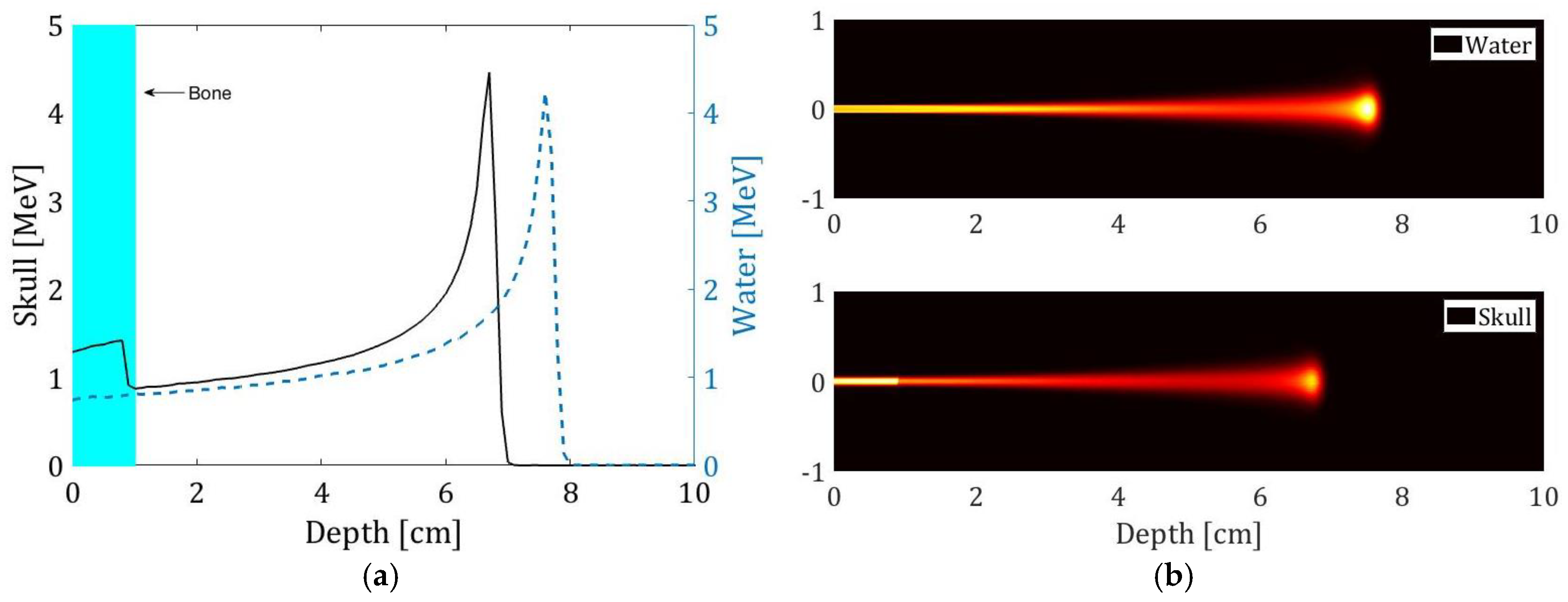
6.1. Energy Deposition

As a result of the interaction of protons with matter following the behavior of the Bragg peak, it is possible to determine the energy deposited in the medium for a 100 MeV proton beam. For this, the deposition in the middle was evaluated directly and with a 1 cm bone layer that simulates the skull following the geometric models of the Geant4 libraries. Thus, Figure 2 shows the Bragg profile as a function of the range in water, with the bone layer described and the distribution of this energy in a plane.

Figure 2 shows the range in water for 100 MeV with and without the skull material.

Figure 2. Energy deposition for a proton beam of 100 MeV with Gauss profile ($\sigma$ = 1 mm) and ${10}^6$ protons. (a) Interaction with the water phantom and with a 1 cm bone layer. (b) Deposition in a plane for 100 MeV; the upper figure shows the phantom water, and the lower one shows the interaction with a layer of bone; the vertical and horizontal units are centimeters.

Figure 2. Energy deposition for a proton beam of 100 MeV with Gauss profile ($\sigma$ = 1 mm) and ${10}^6$ protons. (a) Interaction with the water phantom and with a 1 cm bone layer. (b) Deposition in a plane for 100 MeV; the upper figure shows the phantom water, and the lower one shows the interaction with a layer of bone; the vertical and horizontal units are centimeters.

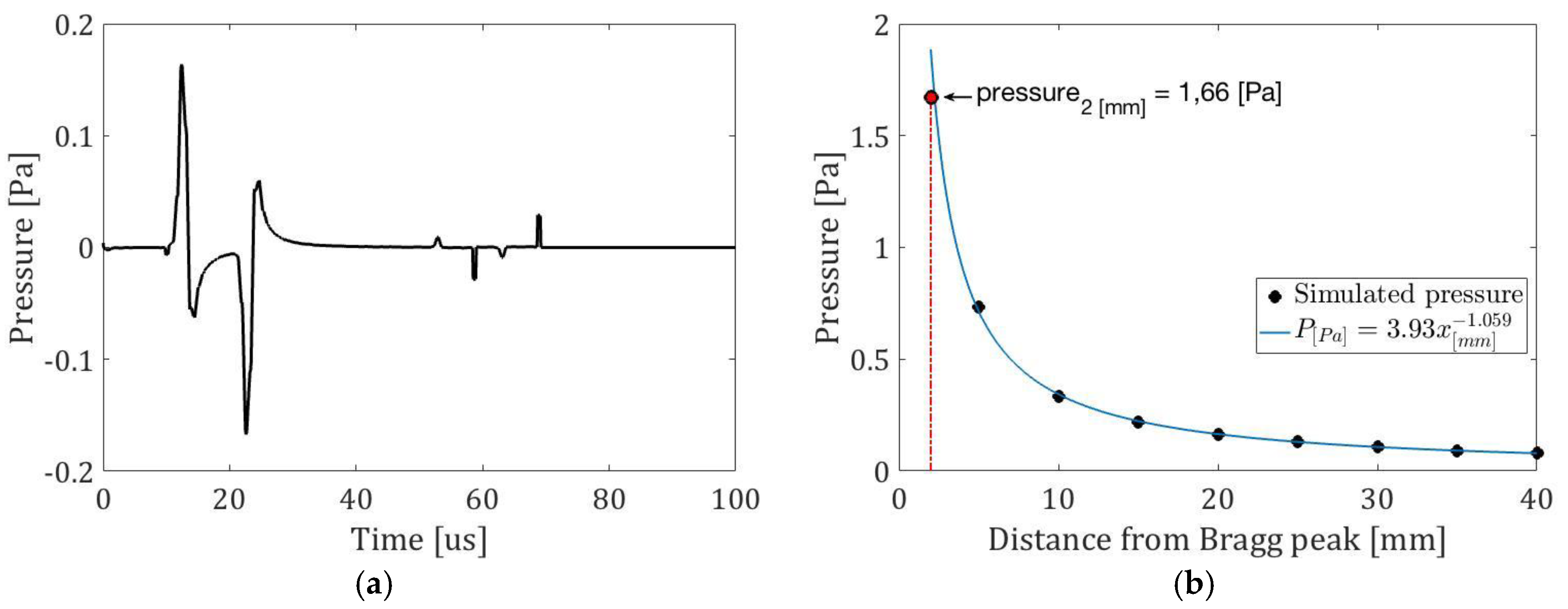
6.2. Thermoacoustic Signal

Because most of the energy was deposited in a volume that had a depth of approximately 2 mm, it was necessary to propagate the pressure from the simulation of different points in the space on the beam emission axis. For this, the pressure received simulated by a 5 mm to 40 mm sensor in 5 mm steps was simulated. For this, the expression $Pp=\frac{P_o}{d}·e^{-\alpha d}$ was used where $P_o$ is a known reference pressure, $d$ the distance between the source and the sensor, and $\alpha$ the water absorption coefficient. With these, Figure 3 shows the pressure signal received by a sensor 20 mm from the Bragg peak, the maximum simulated pressure values for different distances and a setting that establishes a pressure of 1.66 Pa at a distance of 2 mm.

Once the pressure behavior was simulated and established over time, the pressure value at a distance of 2 mm was set in the FEM model for wave propagation at a volume that corresponds to the peak maximum of Bragg shown in Figure 2b.

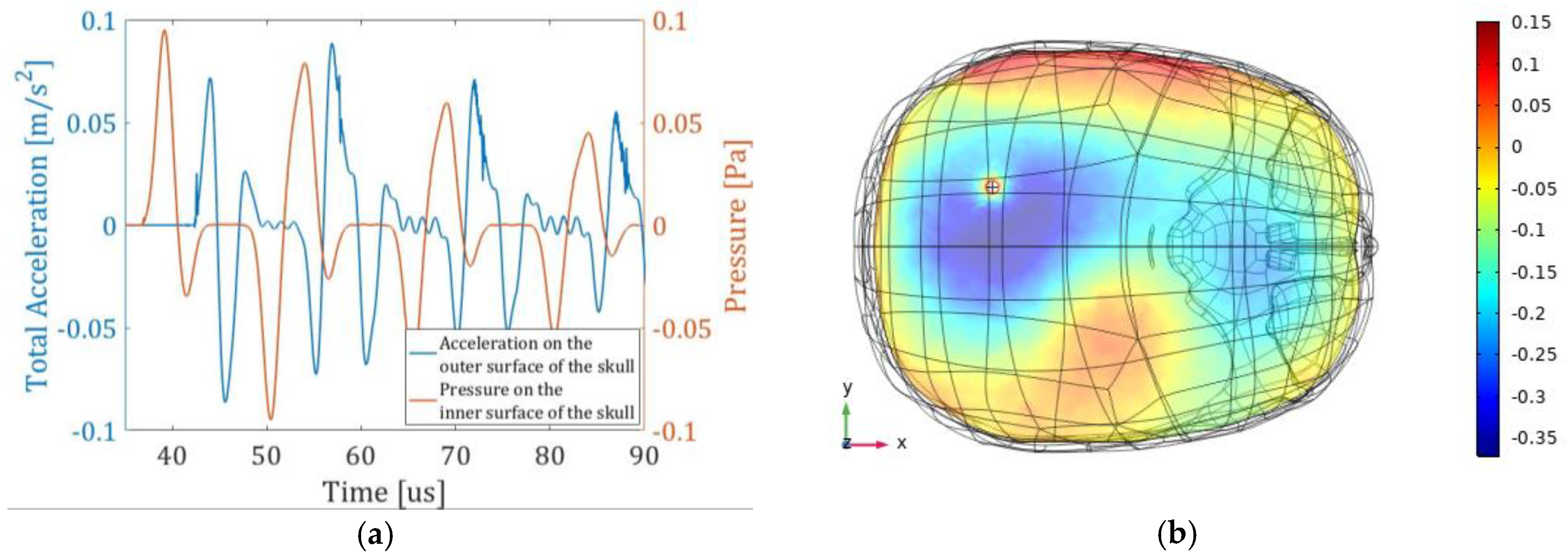
6.3. Acoustic Propagation

Once the acoustic pressure was calculated using the thermoacoustic model and obtaining the pressure propagated to a source whose volume coincides with the energy deposition, the propagation in the brain was performed using the FEM model. For this, a uniform density was taken in the region inside the skull with a value of 1003 $\mathrm{kg}/{\mathrm{m}}^3$ that corresponded to the density of the water since the brain tissue and the cerebrospinal fluid have a similar density [9]. Figure 4 shows an image of the propagation in a horizontal plane in the instant of time $t=53 \mathsf{\mu }\mathrm{s}$. In addition, the pressure signal received on the bone inside the skull and the acceleration on the outside surface of the skull are shown.

The received signal is in terms of the acceleration on the surface of the skull. This signal can be converted to pressure to have a voltage reference due to the Receiving Voltage Response (RVR) of the sensor attached to an adaptation layer. This signal is evaluated in time and correlated with the signal emitted by the source to obtain the time differences of arrival among the sensors (TDOA) which are referenced to one of the sensors. The signal received by the sensors corresponds to an acceleration analysis that delivers the FEM method obtained in one of the outputs in the solid mechanic module. Therefore, each of these signals was evaluated to get the arrival times from the source.

6.4. Acoustic Localization

In the first approach, the signals arrival times were obtained by cross-correlation between the emitted signal (Figure 3a) and the set of received signals. Thus, it was possible to determine the TDOA and solve the system of equations for the $6$ sensor locations tested.

Table 1. Estimated position of the Bragg peak energy deposition.

	Sensor [mm]						Source Position [mm]	Reconstructed Position [mm]
	1	2	3	4	5	6
X	−111.7	−11.1	−10.9	−10.1	−10.1	−100.0	−70.00	−69.20
Y	1.1	13.8	29.8	1.0	15.6	33.5	20.00	20.81
Z	172.2	172.1	171.5	174.0	174.1	173.4	171.90	173.30

shows the positioning of the sensors and the results of the reconstructed position by the location algorithm for energy deposition. It can be seen that there was a deviation between the reconstructed position and the simulated source of about 1.8 mm. However, in a closer approach, this reconstructed position was recalculated by correcting the different sound speed velocity by the skull with respect to the water. The results are also shown in Table 1, noting that the last deviation reduced to 1.0 mm.

The spatial reference for the sensors was given by the software (COMSOL), whereby the position of the source within the skull was known.

7. Conclusions

Studies were conducted on the deposition of energy in brain tissue through simulations with the Monte Carlo methods for the energy of 100 MeV. It was possible to determine the pressure at a point in space by discretizing the thermoacoustic model and propagating the pressure to a size similar to the Bragg peak. Therefore, through sensors located on the surface of the skull, the position of the source was reconstructed from the moment of detection by the different sensors, while also considering the corrections in time due to the change of impedance among the propagation media. The position of the source was solved with few iterations, using a robust resolution method for nonlinear equations. Therefore, this technique can be considered as a good alternative for monitoring the location of the Bragg peak in the treatment of hadron therapy.

References

1. De Ruysscher, D.; Lodge, M.M.; Jones, B.; Brada, M.; Munro, A.; Jefferson, T.; Pijls-Johannesma, M. Charged particles in radiotherapy: A 5-year update of a systematic review. Radiother. Oncol. 2012, 103, 5–7. [Google Scholar] [CrossRef] [PubMed]
2. Database, C.M. International Agency for Research on Cancer. Available online: http://www-dep.iarc.fr/WHOdb/WHOdb.htm (accessed on 18 February 2019).
3. Kraan, A.C.; Battistoni, G.; Belcari, N.; Camarlinghi, N.; Ciocca, M.; Ferrari, A.; Ferretti, S.; Mairani, A.; Molinelli, S.; Pullia, M.; Sala, P. Online monitoring for proton therapy: A real-time procedure using a planar PET system. Nucl. Instrum. Methods Phys. Res. 2015, 786, 120–126. [Google Scholar] [CrossRef]
4. Aso, T.; Kimura, A.; Kameoka, S.; Murakami, K.; Sasaki, T.; Yamashita, T. GEANT4 based simulation framework for particle therapy system. In Proceedings of the IEEE Nuclear Science Symposium Conference Record, Honolulu, HI, USA, 26 October–3 November 2007. [Google Scholar]
5. Sulak, L.; Armstrong, T.; Baranger, H.; Bregman, M.; Levi, M.; Mael, D.; Strait, J.; Bowen, T.; Pifer, A.E.; Polakos, P.A.; et al. Experimental studies of the acoustic signature of proton beams traversing fluid media. Nucl. Instrum. Methods Phys. Res. 1979, 161, 203–217. [Google Scholar] [CrossRef]
6. A. M. U. Guide. Available online: https://doc.comsol.com/5.4/doc/com.comsol.help.aco/AcousticsModuleUsersGuide.pdf (accessed on 2 October 2019).
7. Otero, J.; Felis, I.; Ardid, M.; Herrero, A. Acoustic localization of bragg peak proton beams for hadrontherapy monitoring. Sensors 2019, 19, 1971. [Google Scholar] [CrossRef] [PubMed]
8. Otero, J.; Ardid, M.; Felis, I.; Herrero, A. Acoustic location of Bragg peak for hadrontherapy monitoring. In Proceedings of the 5th International Electronic Conference on Sensors and Applications, ecsa-5.sciforum.net, 15–30 November 2018. [Google Scholar]
9. Barber, T.; Brockway, J.; Higgins, L. The density of tissues in and about the head. Acta Neurol. Scand. 1970, 46, 85–92. [Google Scholar] [CrossRef] [PubMed]
10. Sauer, T. Resolución de Ecuaciones; Análisis numérico; Pearson: London, UK, 2013; pp. 24–71. [Google Scholar]
11. Askaryan, G.A. Hydrodynamic radiation from the tracks of ionizing particles in stable liquids. Sov. J. At. Energy 1957, 3, 921–923. [Google Scholar] [CrossRef]
Figure 1. (a) Position of the sensors where the acceleration produced by the pressure inside the skull was evaluated. (b) Simulated volume and pressure source.
Proceedings 42 00071 g001
Figure 3. (a) Pressure received 20 mm from the Bragg peak on the proton beam emission axis. (b) Simulated pressure in terms of distance.
Proceedings 42 00071 g003
Figure 4. (a) Left axis, signal received on one of the sensors [m/s2] and right axis, pressure on the surface of the skull [Pa]. (b) Signal acoustic propagation in the X, Y plane (units in Pa).
Proceedings 42 00071 g004