Measurement of Environmental Efficiency in the Countries of the European Union with the Enhanced Data Envelopment Analysis Method (DEA) during the Period 2005–2012 ^†

Abstract

In recent years there has been growing interest in measuring the environmental efficiency of the different territories, countries and/or nations. This has led to the development of different methods applied to the evaluation of environmental efficiency such as the Data Envelopment Analysis (DEA) method. This method, supported by different studies, allows measuring relative environmental efficiency and is consolidated as a very reliable method to measure the effectiveness of environmental policies in a specific geographical area. The objective of our study is the calculation of the environmental efficiency of the 28 member countries of the European Union (EU) through the DEA method. We will collect the data regarding the last years in which there are reliable comparative data in all. We will study in reference to them, the results of the environmental policies applied in the different countries, in order to make comparisons between countries and classify them according to their environmental efficiency. Using this, two variants of calculation within the DEA method to compare in a contrasted way the results of environmental efficiency for the 28 countries of the European Union (EU) analyzed and propose possible solutions for improvement. Contributing in this work as main novelty the application of a new variant of the DEA Method, which we will call Improved Analysis Method (MAN) and that aims to agglutinate and assess more objectively, the results of the two DEA methods applied. The results show that there are 14 of the 28 countries that have a high relative environmental efficiency. However, we also find countries with very low environmental efficiency that should improve in the coming years. Coinciding precisely in this last group with countries recently admitted to the EU and where environmental policies have not yet been applied effectively and with positive results.

1. Introduction

The progressive increase of the population, especially in large cities, the depletion of natural resources, the generation of waste and its impact, is having direct consequences on the pollution of the natural environment, causing natural disasters, associated with climate change [1]. All this requires a change on a global scale defining sustainable environmental policies. The rational and sustainable use of natural and energy resources is key to solving this problem. The concept of sustainable development that implies “meeting the needs of the present generation but without compromising the needs of future generations”, now makes more sense than ever. [2].

The II Earth Summit of Rio de Janeiro in 1992, [3], the Kyoto Protocol for the reduction of greenhouse gas emissions [4] until reaching the Paris Agreement in 2015 where the main objective was defined as “strengthening the global response to the threat of climate change, in the context of sustainable development and efforts to eradicate poverty“ (UNFCCC, 2015) [5]. They have provoked an evolution of the concept of sustainable development oriented towards energy efficiency or eco-efficiency.

Eco-efficiency is defined as an attempt to provide goods and services at a competitive price, satisfying human needs and quality of life, by progressively reducing the environmental impact and the intensity of the use of resources throughout the life cycle, up to level compatible with the estimated capacity that the Planet can support [6].

Likewise, the countries of the European Union have established as strategic objectives the “green growth” that implies the development of integrated policies that promote a sustainable environmental framework. (European Union, 2014), protect nature, favor sustainable development based on sustainable economic growth and the protection of the environment. In addition to the H2020 objective (20% reduction of greenhouse gas emissions, 20% of renewable energy, 20% of the improvement of environmental efficiency to achieve these objectives before 2020) [7].

Measuring eco-efficiency is not easy and depends on many factors. However, environmental efficiency data can be obtained using the DEA (Data Envelopment Analysis) method [8].

The DEA method [9], is a method used to calculate the relative efficiency of different units that are called DMUs (decision making units, “decision making units”). For this, they are based on the existence of certain input variables (inputs) that give rise to certain output variables (outputs). Both inputs and outputs are common in the different decision-making units and are assigned certain weights.

Charnes et al. in 1978 they proposed a method to calculate technical efficiency by solving a problem of nonlinear programming. Considering that we have n DMUs denoted as j = (1, 2, …, n) and for each DMU we have m inputs xij (i = 1, 2, …, m) and s outputs yrj (r = 1, 2, …, s), this problem of linear programming can be expressed in the following way [10]:

$$\begin{gathered} {\mathrm{e}}_0=\mathrm{m}\text{á}\mathrm{x} {\sum }_r{u}_r{y}_{ro}/{\sum }_i{v}_i{x}_{io} \\ \mathrm{s}.\mathrm{t}. {\sum }_r{u}_r{y}_{rj}-{\sum }_i{v}_i{x}_{ij}\le 0 \\ {u}_{r,}{v}_i\ge \epsilon \end{gathered}$$

(1)

Being $x_{io}$ the inputs, $y_{ro}$ the outputs, j the set of decision-making units, r the number of outputs, i the number of inputs and $u_r$, and $v_i$ the weights assigned to the outputs and to the inputs, respectively, and $\epsilon$ is a parameter to force the variables to be positive. This method is called CCR by the first letter of the names of its designers [9] and is also known as the CRS (constant retuns to scale) method [10].

However, this problem of non-linear programming can be translated into linear programming in the following way [10]:

$$\begin{gathered} {\mathrm{e}}_0=\max {\sum }_r{\mu }_r{y}_{ro} \\ \mathrm{s}.\mathrm{t}. {\sum }_i{v}_i{x}_{io}=1 \\ {\sum }_r{\mu }_r{y}_{rj}-{\sum }_i{v}_i{x}_{ij}\le 0 \\ {\mu }_{r,}{v}_i\ge \epsilon \end{gathered}$$

(2)

where ${\mu }_r$ = t$u_r$ y $v_i$ = t$v_i$, being t = $({\sum _i{v}_i{x}_{io})}^{-1}$.

After the development of the CRS model, others emerged as:

• RSV (variable returns to scale) [13].
• the additive method [12].
• measures based on slacks-based measures [14].
• the Russell measure (The Russel measure) [15,16,17].
• and other non-radial models, such as RAM (range adjusted measure) [18].

The DEA method has numerous applications for calculating efficiency and since its development has been widely used, becoming more important in recent years. This method can be used in different fields (such as engineering, industry, economics) [19]. It can also be used to calculate environmental efficiency [20,21]. In the DEA-based method for the calculation of environmental efficiency, the output variables or outputs are to be divided into desirable outputs (which we want to be high, for example, income per capita) and undesirable outputs (which suits us that are as low as possible to achieve greater efficiency, for example, contaminants).

The objective of our study is to calculate the environmental efficiency of the 28 member countries of the European Union through the DEA method during the years in which reliable comparative results have been obtained in all the countries analyzed. To be able to study progress in environmental efficiency in different countries and to make comparisons between countries and classify them according to their environmental efficiency. Likewise, different solutions or alternatives will be proposed to improve the situation in the different countries based on the results obtained. We will also use two calculation options within the DEA method to compare the results obtained. Contributing in this work as a novelty an Improved Analysis Method (MAN) that aims to use the results of the two previous methods to improve the final classification in a more objective way.

2. Methodology

In our case study, we used the 28 countries of the European Union as decision-making units. The data of the inputs and outputs to calculate environmental efficiency were taken from 2005 to 2012 because there were no more recent published data from some of the countries, which did not allow us to do a closer study.

The selected inputs have been the production of electricity from coal, petroleum and nuclear origin (all these data expressed in percentages of the total electricity produced in each country), the annual industrial production index (expressed as a percentage) calculated as the average of the twelve indices of monthly industrial production and the volume of vehicles (understood as the number of vehicles that work with fossil fuels in use in each one of the countries). These inputs are shown in Table 1.

In terms of outputs are divided into desirable outputs that are those that will contribute to that country has greater efficiency and the undesirable outputs that are what detract from efficiency in that country. As desirable outputs, GDP and per capita income were taken and, as undesirable outputs, the emissions of CO₂ (carbon dioxide) and CH₄ (methane). The output ratio is shown in Table 1.

Table 1. List of inputs, desirable outputs and undesirable outputs selected for our study.

Inputs	Outputs Desirable	Outputs Undesirable
Production of Electricity from Coal	PIB Gross Domestic Product (GDP)	CO2
Production of Electricity from Petroleum	Rent per Capita	CH4
Production of Electricity of Nuclear Origin
Industrial Production Index
Volume of Vehicles

Table 1. List of inputs, desirable outputs and undesirable outputs selected for our study.

Inputs	Outputs Desirable	Outputs Undesirable
Production of Electricity from Coal	PIB Gross Domestic Product (GDP)	CO2
Production of Electricity from Petroleum	Rent per Capita	CH4
Production of Electricity of Nuclear Origin
Industrial Production Index
Volume of Vehicles

Taking previous studies as an example, on the one hand, CO₂ emissions were selected as undesirable outputs [8] and CH₄ [22], because they are greenhouse gases that have a large incidence on climate change and higher values of these indicators reduce environmental efficiency. On the other hand, the Gross Domestic Product (GDP) [23] and per capita income [24] were taken as desirable outputs. Both are economic indicators and that account for the economic situation of a country. Therefore, they will have greater environmental efficiency when these values are higher and lower those of emissions, since it would mean that the economic activities carried out are efficient and obtain more benefits but with fewer emissions. As for the inputs that can lead to both positive and negative outputs are the generation of electricity from coal and oil, the generation of electricity from nuclear sources [25], the volume of vehicles and industrial production [26]. The larger these inputs are, the greater will also be the outputs. However, a balance has to be found because, although it is important that GDP and per capita income (our desirable outputs) are high, emissions (our undesirable outputs) should be as low as possible in order to be eco-efficient.

Data on GDP, per capita income, industrial production index, vehicle volume, CO₂ emissions were obtained from the National Statistics Institute of Spain (INE) [27], the National Statistics Institute of Germany (Statistisches Bundesamt) [28], the National Institute of Statistics Statistics of France (INSEE) [29], the European Statistical Office (Eurostat, the Statistical Office of the European Communities) [30], the IMF [31], the World Bank [32], the World Trade Organization [33], the European Central Bank [34], the Bank of Spain [35], the Institute National Statistical Office of Italy (Istat, L’Istituto nazionale di statistica) [36] and the Central Bank of England (Bank of England) [37], while data on the production of electricity from petroleum, coal, nuclear origin and CH₄ emissions extracted from the World Bank’s online database [32].

Once these data were obtained, a statistical study was carried out (taking data from all countries and for all years together) by calculating the mean, maximum, minimum and standard deviation in order to have greater precision in the final evaluation process. The values obtained are shown in

Table 2. Statistical study of inputs and outputs for 28 countries of the EU, 2005–2012. Source: self-made.

	Indicator	Unity	Maximum	Mínimum	Average	Typical Deviation
Inputs	Generation of Electricity from Coal	%	95,709	0	26,918	25,028
	Generation of Electricity from Petroleum	%	100	0,016	10,005	25,127
	Generation of Electricity from Nuclear Energy	%	79,512	0	18,924	23,105
	Industrial Production Index	%	22,842	−23,442	1085	7421
	Traffic Volume	Vehículos	49,742,000	252,000	9,805,492,103	1,362,752,668
Outputs Deseables	PIB (GDP)	Millones de €	2,758,260	5142	454236,517	688,213,992
	Rent per Cápita	€	83,100	3100	23768,5803	15,550,584
Outputs Indeseables	CO2 Emissions	Kts	844,435	2432	142,200,227	190,781,005
	CH4 Emissions	Kt de Equivalente de CO2	837,569	1,409,427	18,849,737	22,216,665

.

Once the statistical study was carried out for all the countries as a whole, the environmental efficiency was calculated for each of the different countries in the years of study. To calculate the efficiency, the two DEA method options [8] were used to compare the two methods in the same way as in the aforementioned article. The theoretical description of both methods is shown below.

2.1. Method 1

We assume that there are k = 1, 2, 3, …, 28 DMUs (Decision Making Units) that correspond to the 28 countries of the European Union. For each of the DMUk we will have N inputs xk = (x1k, x2k, …, xNk), M desirable outputs yk = (y1k, y2k, yMk) and J undesirable outputs uk = (u1k, u2k, … uJk). With all these data we proceed to operate with them in the following way [38]:

$$\begin{gathered} \mathit{EEI}=\min \lambda \\ \mathrm{s}.\mathrm{t}. {\sum }_{k=1}^k{z}_k{x}_{nk}\le x_n, n=1, 2, \dots , \mathrm{N} \\ {\sum }_{k=1}^k{z}_k{y}_{mk}\ge y_m, m=1, 2, \dots , \mathrm{M} \\ {\sum }_{k=1}^k{z}_k{u}_{jk}=\lambda u_{j,} j=1, 2, \dots , \mathrm{J} \\ {z}_k\ge 0, k=1, 2, \dots , \mathrm{K} \end{gathered}$$

(3)

Being EEI the environmental efficiency (Environmental Efficiency Index); K, the number of DMUs; N, the number of inputs; x, the inputs; y, the desirable outputs; M, the number of desirable outputs; z, the undesirable outputs; and j, the number of undesirable outputs.In this way, EEI would be obtained for each of the DMUs. DMUs that have higher EEI will have greater environmental efficiency.

To carry out these calculations, the Solver tool of the Excel program was used, taking as an example an example collected in chapter 2 of W.D. Cook and Joe Zhu, Data Envelopment Analysis: Modeling Operational Processes and Measuring Productivity [11] but modified to meet our needs, since the example that was taken as a model did not include undesirable outputs and it was also necessary to change the restrictions to fit the model shown in Equation 3.

Once the efficiency results were obtained in the different years, the average of the different countries was calculated. Subsequently, the data obtained was analyzed.

2.2. Method 2

In the method we have used so far (Method 1) it is considered that all undesirable inputs have the same importance. However, there are other methods in which undesirable inputs are given different importance. One of these methods is that proposed by Zhou et al. in 2017 [8] (which from now on we will call Method 2) in which different weights are assigned to the undesirable inputs according to their importance and which is described as follows:

$$\begin{gathered} {\mathit{EEI}}_2= \min {\sum }_{j=1}^J{w}_j{\mathsf{\lambda }}_j \\ \mathrm{s}.\mathrm{t}. {\sum }_{k=1}^K{z}_k{\mathrm{x}}_{nk}\le {\mathrm{x}}_n, n=1,2,\dots ,N \\ {\sum }_{k=1}^K{z}_k{\mathrm{y}}_{mk}\ge y_m, m=1,2,\dots ,\mathrm{M} \\ {\sum }_{k=1}^K{z}_k{u}_{jk}\le {\mathsf{\lambda }}_j{\mathrm{u}}_j, j=1,2,\dots ,\mathrm{J} \\ {z}_k\ge 0, {\mathsf{\lambda }}_j\le 1, k=1,2,\dots ,\mathrm{K}, j=1,2,\dots ,\mathrm{J} \end{gathered}$$

(4)

where $w_j(j=\mathrm{1,2},\dots ,J)$ they are the weights that are given to the undesirable inputs.

Using the Excel Solver tool again [11], we obtained the new efficiency values for the 28 countries in these 8 years and proceeded to their interpretation.

3. Results

3.1. Method 1

Once Method 1 was applied to measure environmental efficiency, environmental efficiency data were obtained for the 28 countries of the European Union during the years from 2005 to 2012. [39]. These results are shown in

Table 3. Environmental efficiency data for the 28 countries of the European Union during the 2005–2012 period obtained with the DEA Method 1. Source: own calculations.

	2005	2006	2007	2008	2009	2010	2011	2012
Germany	1	1	1	1	1	1	1	1
Austria	1	1	1	1	1	1	1	1
Belgium	1	1	0.91974	0.90943	1	1	0.91808	0.9181
Bulgaria	0.19318	0.19312	0.18073	0.19388	0.25535	1	0.19434	0.58077
Cyprus	1	1	1	1	1	1	1	1
Croatia	0.55502	0.57879	0.51608	0.54401	0.55786	1	1	1
Denmark	1	1	1	1	1	1	1	1
Slovakia	1	0.34476	0.3937	0.44765	0.4817	0.49112	0.45281	0.43873
Slovenia	0.64194	0.62028	0.6022	0.57549	0.69106	1	0.80081	0.6149
Spain	0.78143	0.78112	0.77369	0.84181	1	1	0.81044	1
Estonia	0.63667	0.68943	0.53955	0.57273	1	0.5902	0.56159	1
Finland	1	0.56014	0.57224	0.61133	0.69907	1	0.58454	0.55831
France	1	1	1	1	1	1	1	1
Greece	1	1	1	1	1	1	1	0.54241
Hungary	0.39984	0.38055	0.40296	0.42662	0.49486	0.39354	0.36761	0.34726
Ireland	1	1	1	1	1	1	1	1
Italy	1	1	1	1	1	1	1	1
Latvia	1	1	1	1	1	1	1	1
Lithuania	1	1	0.63402	1	1	1	1	1
Luxembourg	1	1	1	1	1	1	1	1
Malt	1	1	1	1	1	1	1	1
Netherlands	1	1	1	1	1	1	1	1
Poland	1	1	1	1	1	1	1	1
Portugal	0.59589	1	1	1	0.70056	1	1	1
UK	1	1	1	1	1	1	1	1
Czech Republic	0.28101	0.29438	0.30624	0.3564	0.35152	0.38802	0.33825	0.3137
Romania	1	0.20547	0.22566	0.23233	0.30254	1	0.23183	0.22111
Sweden	1	1	1	1	1	1	1	1

. It must be taken into account that the results obtained are relative environmental efficiency, which means that if there are countries that have 100% efficiency does not mean that their environmental efficiency is perfect, but are the most efficient among the countries we are studying.

Subsequently, we proceeded to calculate the average of the values of environmental efficiency for each of the 28 countries during the 8 years of study (2005–2012). The results are shown in

Table 4. Average environmental efficiency data for the 28 countries in the period 2005–2012 obtained with the DEA Method 1. Source: own calculations.

	Method 1
Germany	1
Austria	1
Belgium	0.95817
Bulgaria	0.34892
Cyprus	1
Croatia	0.71897
Denmark	1
Slovakia	0.50631
Slovenia	0.69333
Spain	0.87356
Estonia	0.69877
Finland	0.6982
France	1
Greece	0.9428
Hungary	0.40165
Ireland	1
Italy	1
Latvia	1
Lithuania	0.95425
Luxembourg	1
Malt	1
Netherlands	1
Poland	1
Portugal	0.91205
UK	1
Czech Republic	0.32869
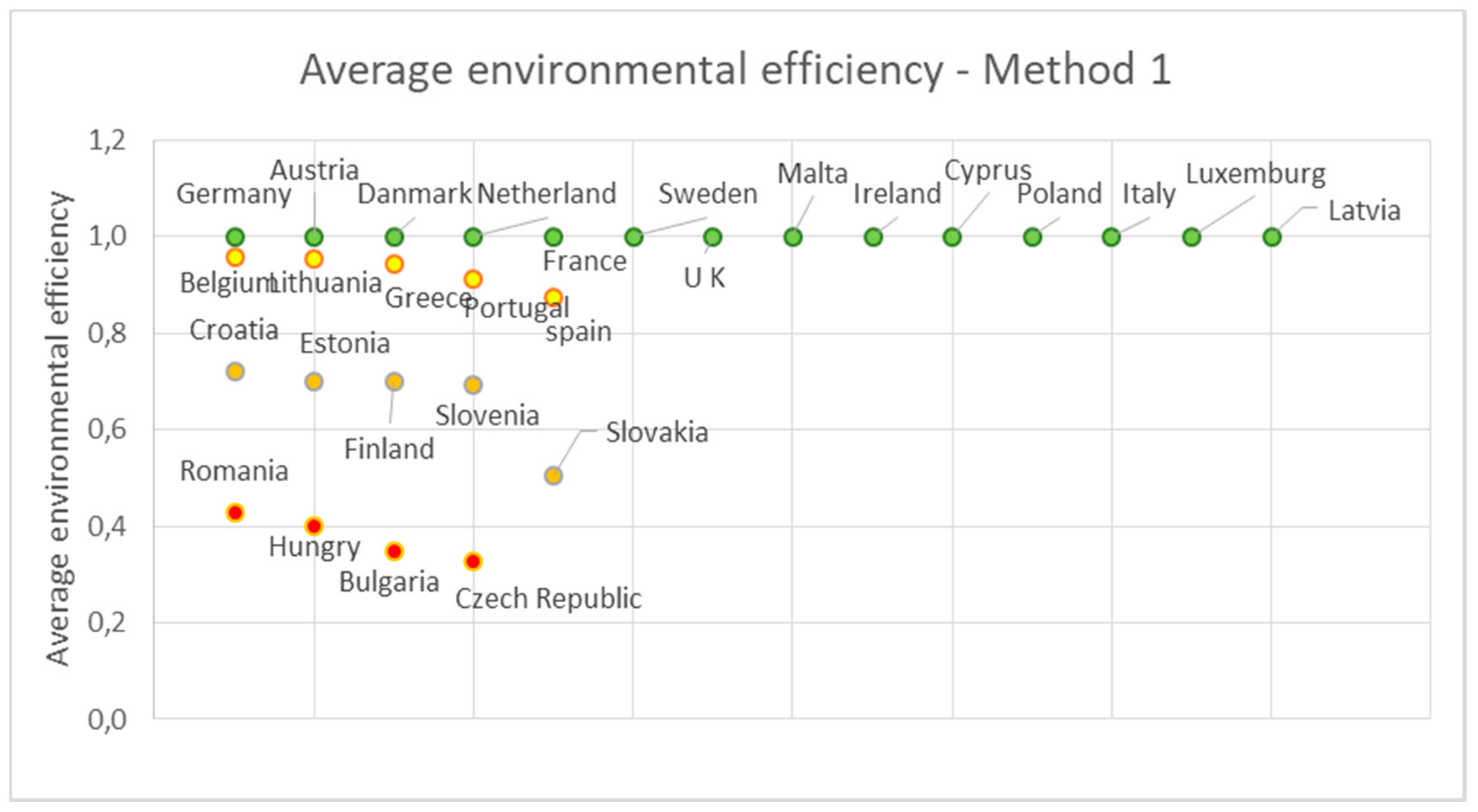
Romania	0.42737
Sweden	1

.

3.2. Method 2

Once the Method 1 is applied and the data obtained for this method is obtained, the environmental efficiencies are calculated, using Method 2 in this case for the later comparison of the two methods. Method 2 differs from 1 in that undesirable inputs are given different weight. In our case, we give a value of 1 to CO₂ and a value of 35 to CH₄ because CH₄ contributes 35 times more than CO₂ in global warming [40]. The efficiency results with Method 2 can be found in

Table 5. Environmental efficiency values for the 28 countries (2005–2012) obtained with Method 2. Source: own calculations.

Method 2	2005	2006	2007	2008	2009	2010	2011	2012
Germany	1	1	1	1	1	1	1	1
Austria	1	1	1	1	1	1	1	1
Belgium	0.98893	0.95715	0.8916	0.87118	0.94409	0.88882	0.8871	0.88412
Bulgaria	0.08567	0.08791	0.09166	0.09607	0.16249	1	0.10569	0.10154
Cyprus	0.91388	1	0.92983	0.97352	1	1	1	1
Croatia	0.27692	0.26546	0.26547	0.28589	0.29653	1	1	0.38745
Denmark	1	1	1	1	1	1	1	1
Slovakia	1	0.33362	0.38596	0.44111	0.47296	0.49098	0.44371	0.42889
Slovenia	0.36179	0.36746	0.38247	0.39883	0.57175	1	0.43572	0.42127
Spain	0.74073	0.70968	0.71636	0.70626	1	1	0.64551	1
Estonia	0.48067	0.48782	0.49582	0.50994	1	0.53298	0.54701	0.51749
Finland	1	0.5064	0.49674	0.50087	0.68142	1	0.54721	0.51542
France	1	1	1	1	1	1	1	1
Greece	1	1	0.68915	0.7002	0.70334	1	1	0.52688
Hungary	0.34526	0.3281	0.35654	0.37236	0.49103	0.35305	0.34391	0.32601
Ireland	0.43603	1	1	0.41988	0.39115	0.37938	1	0.35505
Italy	1	1	1	1	1	1	1	1
Latvia	0.3715	0.36776	0.37698	0.3866	1	1	1	1
Lithuania	0.22283	0.2231	0.22836	0.22883	0.25729	1	0.25265	0.24597
Luxembourg	1	1	1	1	1	1	1	1
Malt	1	1	1	1	1	1	1	1
Netherlands	1	1	1	1	1	1	1	1
Poland	1	1	1	1	0.12434	0.13739	0.13727	1
Portugal	0.34108	1	0.42332	0.34787	0.36575	0.54239	0.47781	1
UK	1	1	1	1	1	1	1	1
Czech Republic	0.26539	0.27826	0.29203	0.33118	0.33438	0.37275	0.32031	0.2987
Romania	1	1	0.12978	0.14137	0.13375	0.18142	0.12784	0.1234
Sweden	1	1	1	1	1	1	1	1

.

The values of average environmental efficiency of each of the countries were also obtained with the data obtained with Method 2. The results are shown in

Table 6. Average environmental efficiency data for the 28 countries in the period 2005–2012 obtained with the DEA Method 2. Source: own calculations.

	Méthod 2
Germany	1
Austria	1
Belgium	0.91412
Bulgaria	0.21638
Cyprus	0.97715
Croatia	0.47221
Denmark	1
Slovakia	0.49965
Slovenia	0.49241
Spain	0.81481
Estonia	0.57147
Finland	0.65601
France	1
Greece	0.82744
Hungary	0.36453
Ireland	0.62268
Italy	1
Letonia	0.68785
Lituania	0.33238
Luxemburgo	1
Malta	1
Países Bajos	1
Polonia	0.67487
Portugal	0.56228
Reino Unido	1
República Checa	0.31162
Rumanía	0.35469
Suecia	1

.

4. Discussion of Results

4.1. Statistical Study of Inputs and Outputs Data

Once the data of the statistical analysis was obtained, which was done with all the input and output data for the 28 countries and in the selected years jointly, the results of the analysis were analyzed [41].

• As for the generation of electricity from coal, the maximum value is reached in Estonia in the year 2007 while the lowest value is repeated in different countries for several years, as for example in Malta, Cyprus, Latvia and Luxembourg during the years 2005 and 2006, among others.
• For the generation of electricity from oil, the highest value is reached in Malta for several years, for example, in 2005 or in 2008. The lowest value is reached in Latvia in 2012.
• In the generation of electricity from nuclear energy, we have that the highest value is reached in 2011 in France. As for the minimum value, this is reached on several occasions in several countries although they are often repeated. For example, this value is achieved in Austria, Cyprus, Croatia, Denmark, Estonia, Greece, Ireland, Italy, Latvia, Luxembourg, Malta, Poland and Portugal in 2007 and 2008, among others.
• The maximum value of the industrial production index is given in 2010 in Estonia. However, the lowest value was also reached in Estonia in 2009.
• Regarding the volume of vehicles, the maximum value is found in Germany in 2006 and the lowest value in Malta in the year 2005.
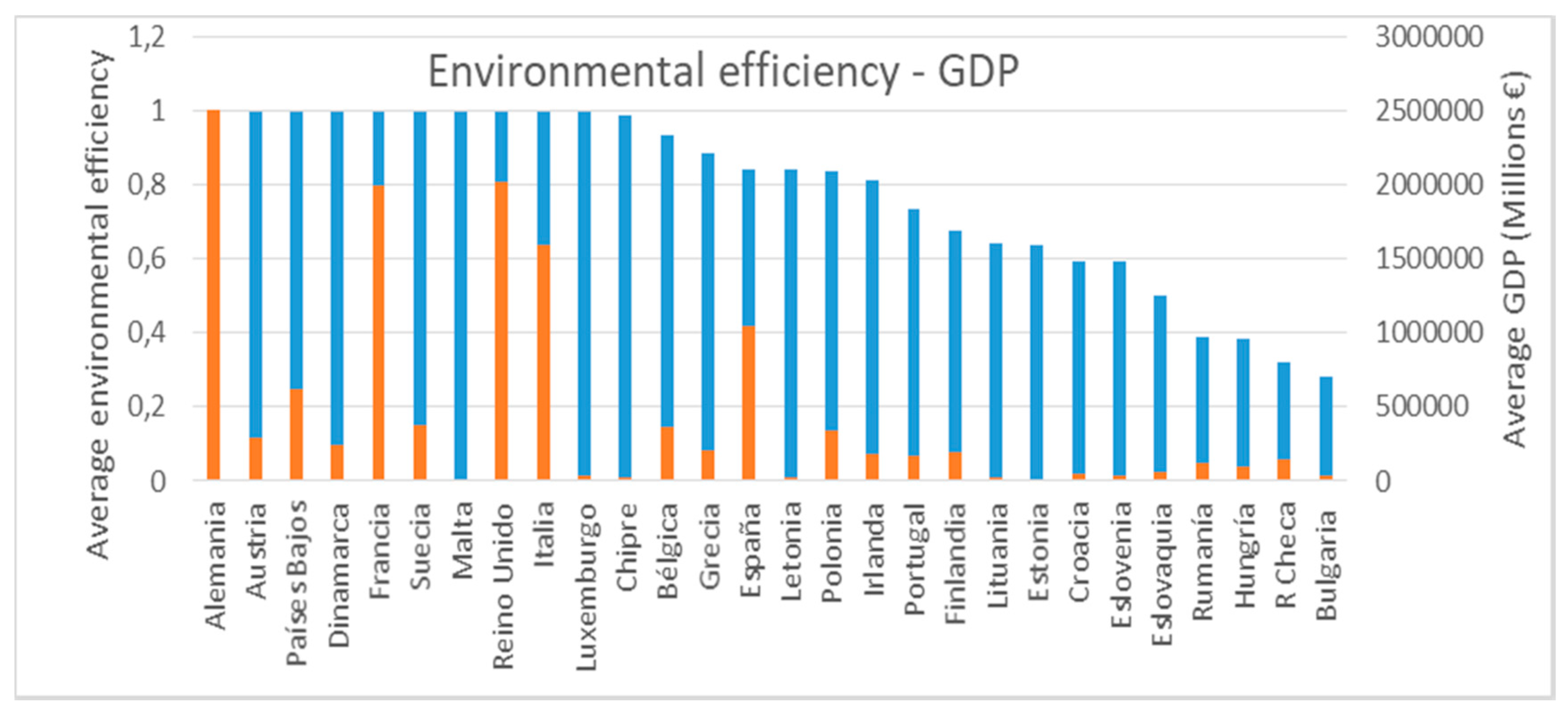
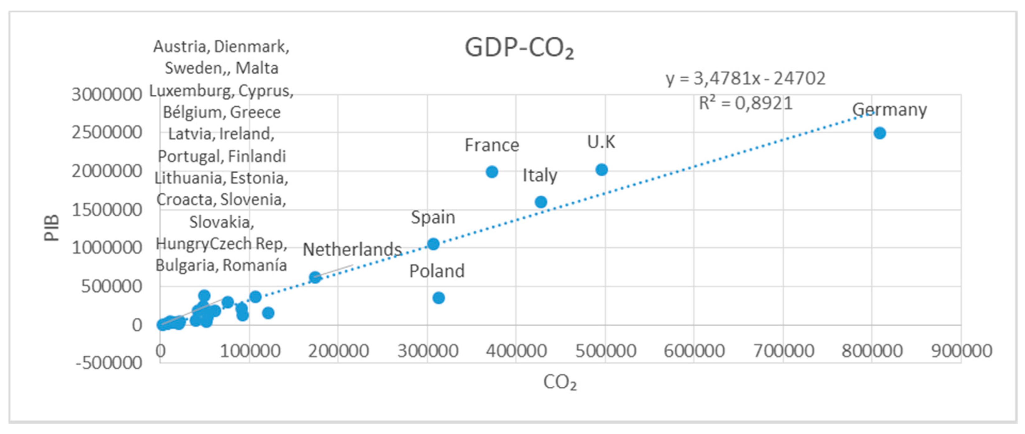
• For GDP, the highest value is reached in 2012 in Germany. The lowest value is reached in Malta in the year 2005.
• In per capita income, the highest value is reached in Luxembourg in 2011 while the lowest value is reached in 2005 in Bulgaria.
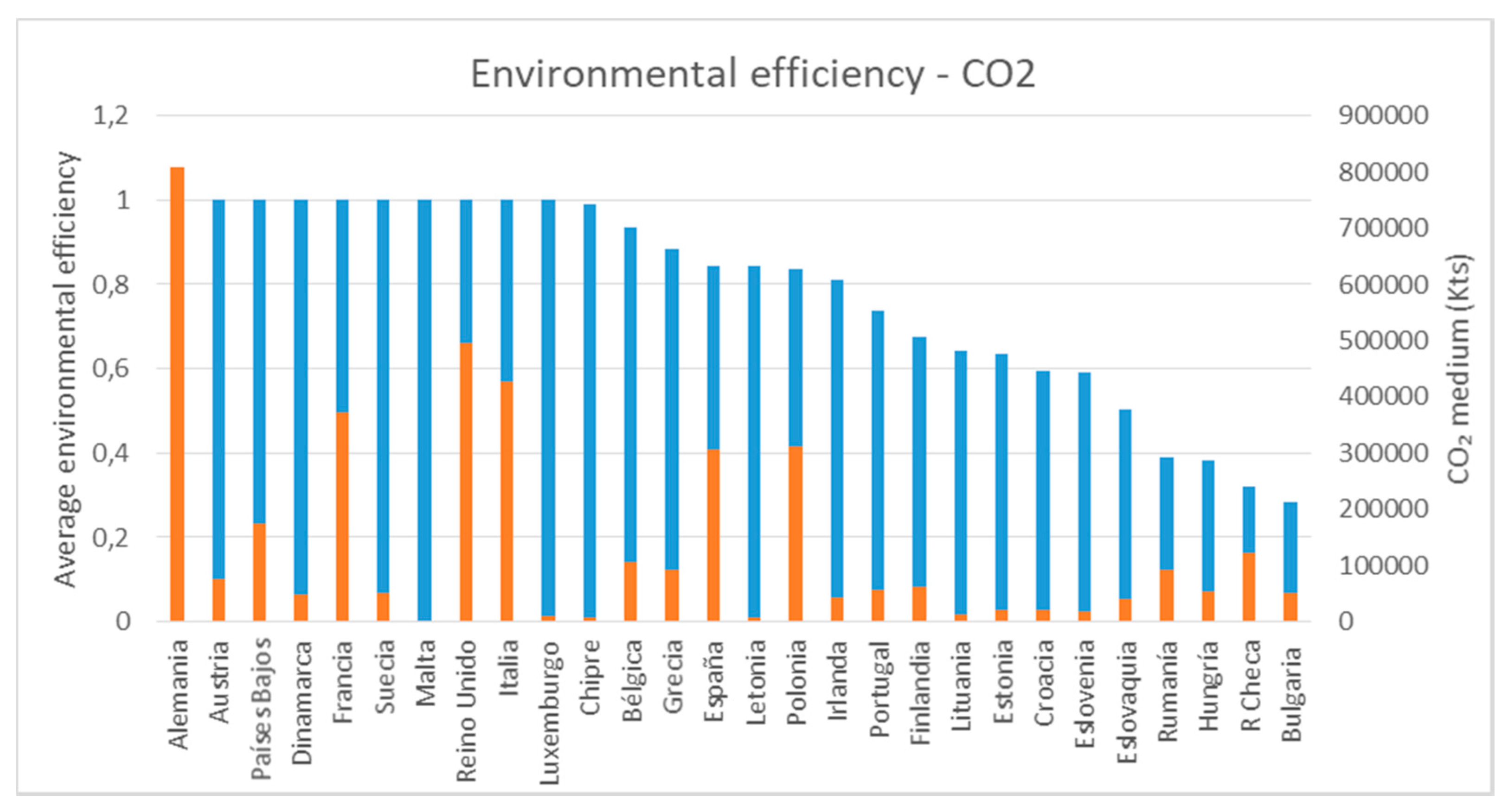
• In carbon dioxide emissions, the highest value is found in 2006 in Germany and the lowest value in Luxembourg in 2012.
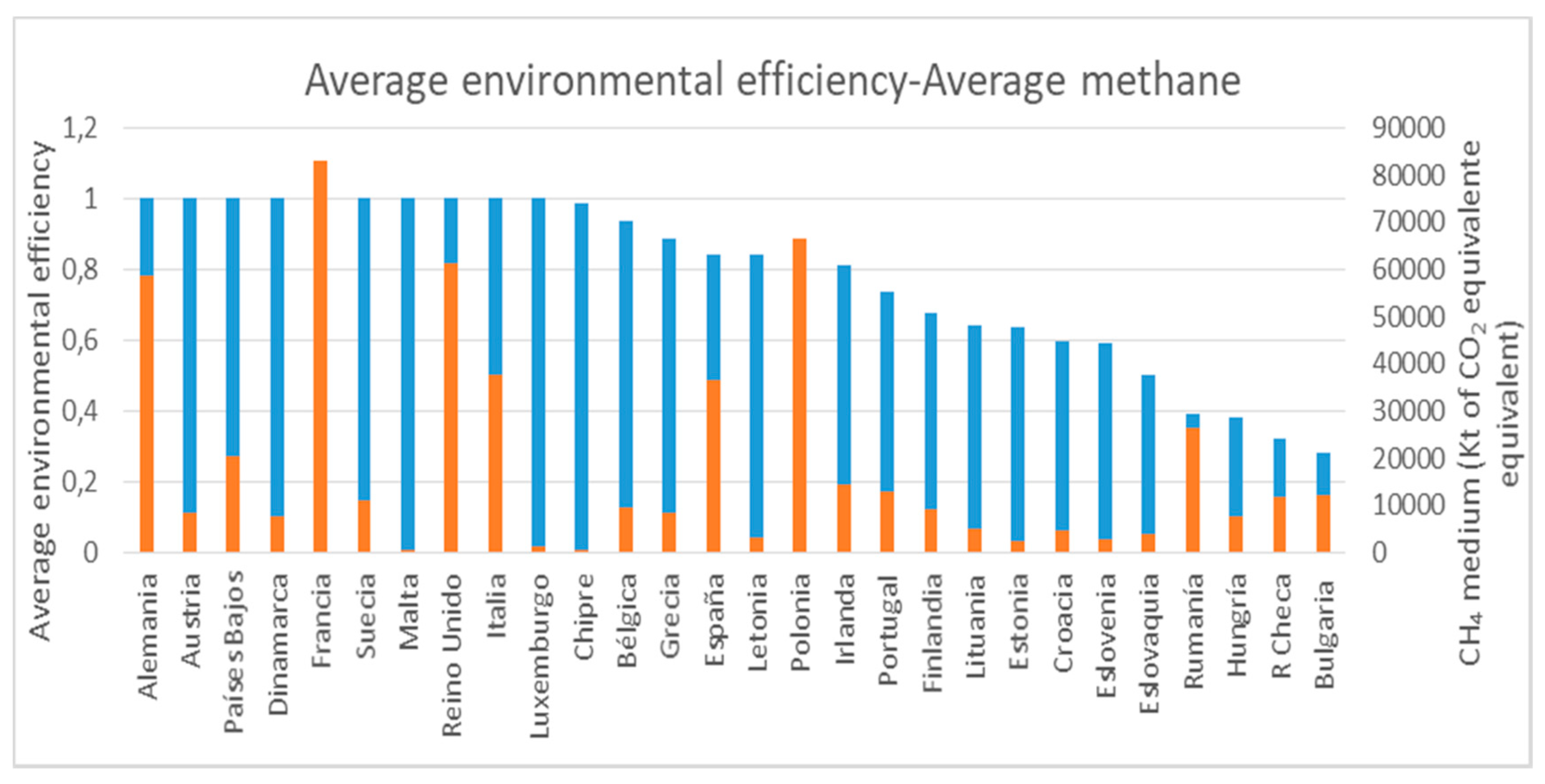
• For methane emissions, the highest value was reached in 2010 in France. However, the lowest value was reached in Luxembourg in 2012.

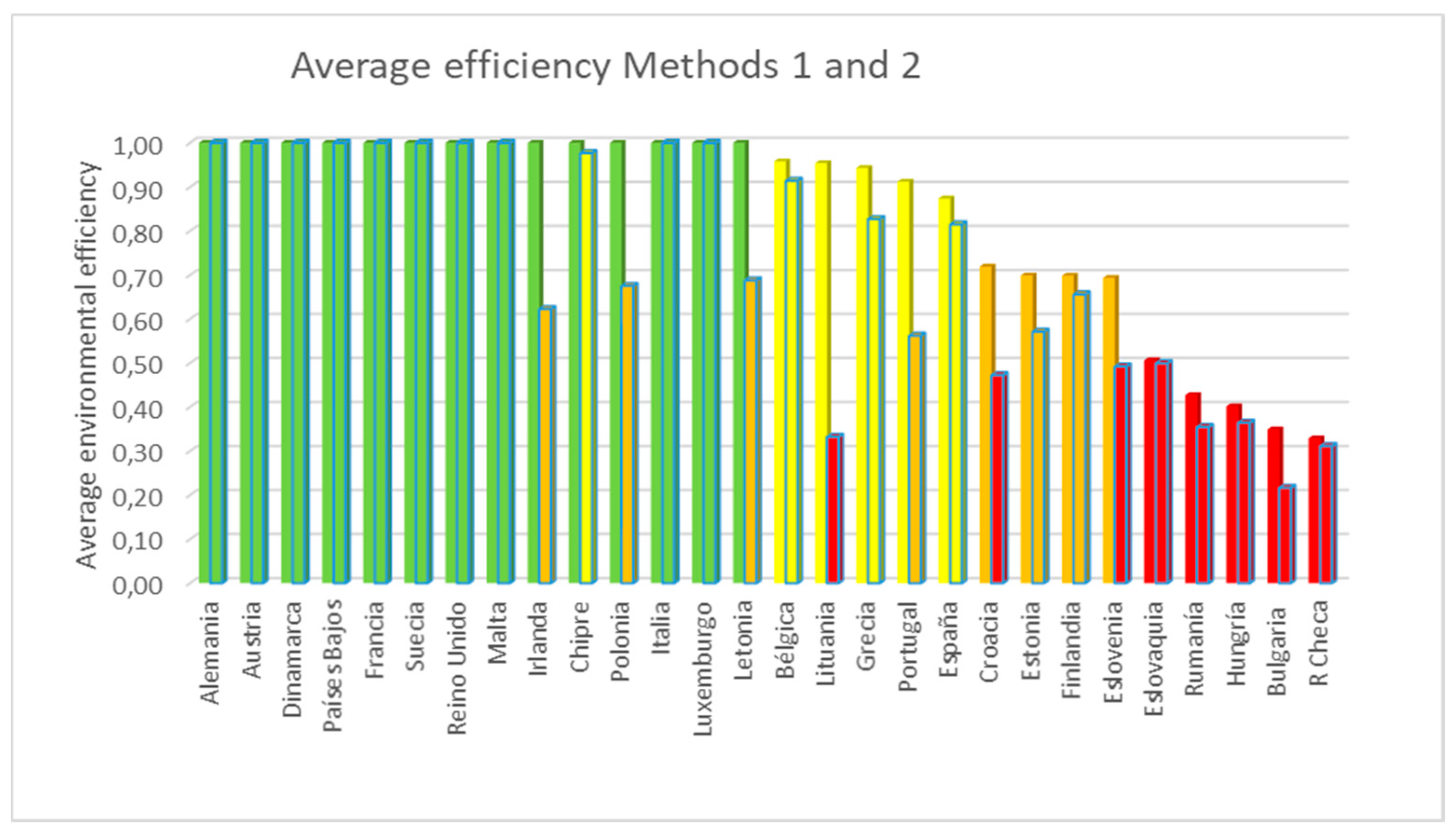
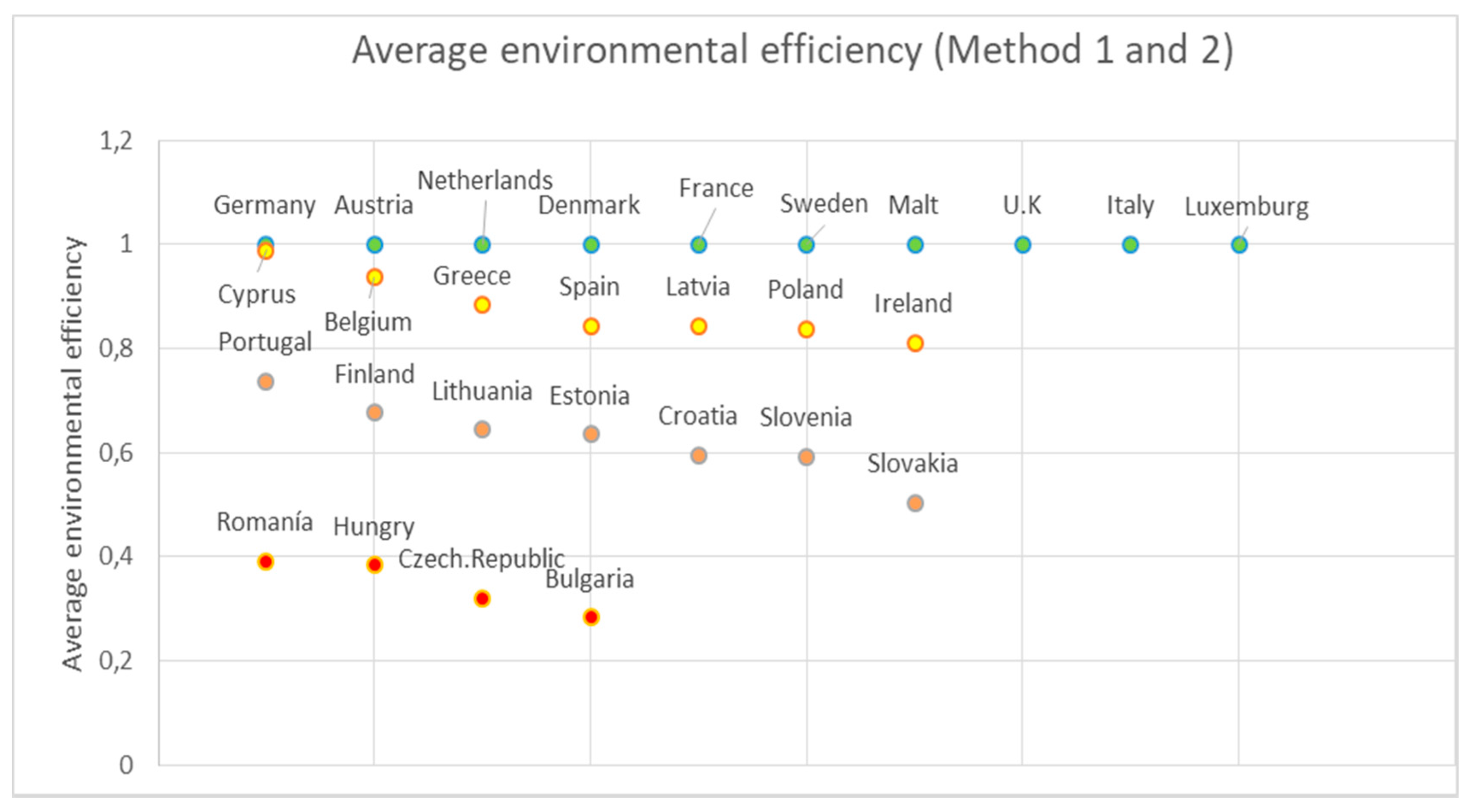
4.2. Comparison between Method 1 and Method 2

Once we have the relative environmental efficiency data obtained by each of the two methods, we compare the results obtained. The data is shown in

Table 7. Comparison of environmental efficiencies with Method 1 and with Method 2 for the 28 countries in the period 2005–2008. Source: self made.

	2005		2006		2007		2008
	Method 1	Method 2	Method 1	Method 2	Method 1	Method 2	Method 1	Method 2
Germany	1	1	1	1	1	1	1	1
Austria	1	1	1	1	1	1	1	1
Belgium	1	0.98893	1	0.95715	0.91974	0.8916	0.90943	0.87118
Bulgaria	0.19318	0.08567	0.19312	0.08791	0.18073	0.09166	0.19388	0.09607
Cyprus	1	0.91388	1	1	1	0.92983	1	0.97352
Croatia	0.55502	0.27692	0.57879	0.26546	0.51608	0.26547	0.54401	0.28589
Denmark	1	1	1	1	1	1	1	1
Slovakia	1	1	0.34476	0.33362	0.3937	0.38596	0.44765	0.44111
Slovenia	0.64194	0.36179	0.62028	0.36746	0.6022	0.38247	0.57549	0.39883
Spain	0.78143	0.74073	0.78112	0.70968	0.77369	0.71636	0.84181	0.70626
Estonia	0.63667	0.48067	0.68943	0.48782	0.53955	0.49582	0.57273	0.50994
Finland	1	1	0.56014	0.5064	0.57224	0.49674	0.61133	0.50087
France	1	1	1	1	1	1	1	1
Greece	1	1	1	1	1	0.68915	1	0.7002
Hungary	0.39984	0.34526	0.38055	0.3281	0.40296	0.35654	0.42662	0.37236
Ireland	1	0.43603	1	1	1	1	1	0.41988
Italy	1	1	1	1	1	1	1	1
Latvia	1	0.3715	1	0.36776	1	0.37698	1	0.3866
Lithuania	1	0.22283	1	0.2231	0.63402	0.22836	1	0.22883
Luxembourg	1	1	1	1	1	1	1	1
Malt	1	1	1	1	1	1	1	1
Netherlands	1	1	1	1	1	1	1	1
Poland	1	1	1	1	1	1	1	1
Portugal	0.59589	0.34108	1	1	1	0.42332	1	0.34787
UK	1	1	1	1	1	1	1	1
Czech Republic	0.28101	0.26539	0.29438	0.27826	0.30624	0.29203	0.3564	0.33118
Romania	1	1	0.20547	1	0.22566	0.12978	0.23233	0.14137
Sweden	1	1	1	1	1	1	1	1

and

Table 8. Comparison of environmental efficiencies with Method 1 and with Method 2 for the 28 countries in the 2009–2012 period. Source: self made.

	2009		2010		2011		2012
	Method 1	Method 2	Method 1	Method 2	Method 1	Method 2	Method 1	Method 2
Germany	1	1	1	1	1	1	1	1
Austria	1	1	1	1	1	1	1	1
Belgium	1	0.94409	1	0.88882	0.91808	0.8871	0.90943	0.88412
Bulgaria	0.25535	0.16249	1	1	0.19434	0.10569	0.19388	0.10154
Cyprus	1	1	1	1	1	1	1	1
Croatia	0.55786	0.29653	1	1	1	1	0.54401	0.38745
Denmark	1	1	1	1	1	1	1	1
Slovakia	0.4817	0.47296	0.49112	0.49098	0.45281	0.44371	0.44765	0.42889
Slovenia	0.69106	0.57175	1	1	0.80081	0.43572	0.57549	0.42127
Spain	1	1	1	1	0.81044	0.64551	0.84181	1
Estonia	1	1	0.5902	0.53298	0.56159	0.54701	0.57273	0.51749
Finland	0.69907	0.68142	1	1	0.58454	0.54721	0.61133	0.51542
France	1	1	1	1	1	1	1	1
Greece	1	0.70334	1	1	1	1	1	0.52688
Hungary	0.49486	0.49103	0.39354	0.35305	0.36761	0.34391	0.42662	0.32601
Ireland	1	0.39115	1	0.37938	1	1	1	0.35505
Italy	1	1	1	1	1	1	1	1
Latvia	1	1	1	1	1	1	1	1
Lithuania	1	0.25729	1	1	1	0.25265	1	0.24597
Luxembourg	1	1	1	1	1	1	1	1
Malt	1	1	1	1	1	1	1	1
Netherlands	1	1	1	1	1	1	1	1
Poland	1	0.12434	1	0.13739	1	0.13727	1	1
Portugal	0.70056	0.36575	1	0.54239	1	0.47781	1	1
UK	1	1	1	1	1	1	1	1
Czech Republic	0.35152	0.33438	0.38802	0.37275	0.33825	0.32031	0.3564	0.2987
Romania	0.30254	0.13375	1	0.18142	0.23183	0.12784	0.23233	0.1234
Sweden	1	1	1	1	1	1	1	1

.

As a general rule, with Method 2, efficiency values tend to be lower than in Method 1, since by giving greater weight to methane emissions, countries that had high methane emissions but low CO₂ emissions have less efficiency by giving more importance to methane emissions, in some cases leading to much lower efficiency (for example, in the case of Ireland where its efficiency for 2005 in Method 1 is 1 and in Method 2 it is of 0.436).

Subsequently, we proceeded to compare the average environmental efficiency values obtained for each of the methods. The results are shown in

Table 9. Values of average environmental efficiency with Method 2 and with Method 1 for the 28 countries in the period 2005–2012. Source: self made.

	Method 1	Method 2
Germany	1	1
Austria	1	1
Belgium	0.95817	0.91412
Bulgaria	0.34892	0.21638
Cyprus	1	0.97715
Croatia	0.71897	0.47221
Denmark	1	1
Slovakia	0.50631	0.49965
Slovenia	0.69333	0.49241
Spain	0.87356	0.81481
Estonia	0.69877	0.57147
Finland	0.6982	0.65601
France	1	1
Greece	0.9428	0.82744
Hungary	0.40165	0.36453
Ireland	1	0.62268
Italy	1	1
Latvia	1	0.68785
Lithuania	0.95425	0.33238
Luxembourg	1	1
Malt	1	1
Netherlands	1	1
Poland	1	0.67487
Portugal	0.91205	0.56228
UK	1	1
Czech Republic	0.32869	0.31162
Romania	0.42737	0.35469
Sweden	1	1

.

As we have seen before in the absolute values, in the average values for the different countries one can also see how the values of average environmental efficiency tend to be lower with Method 2, giving greater importance to methane than to carbon dioxide in the undesirable inputs.

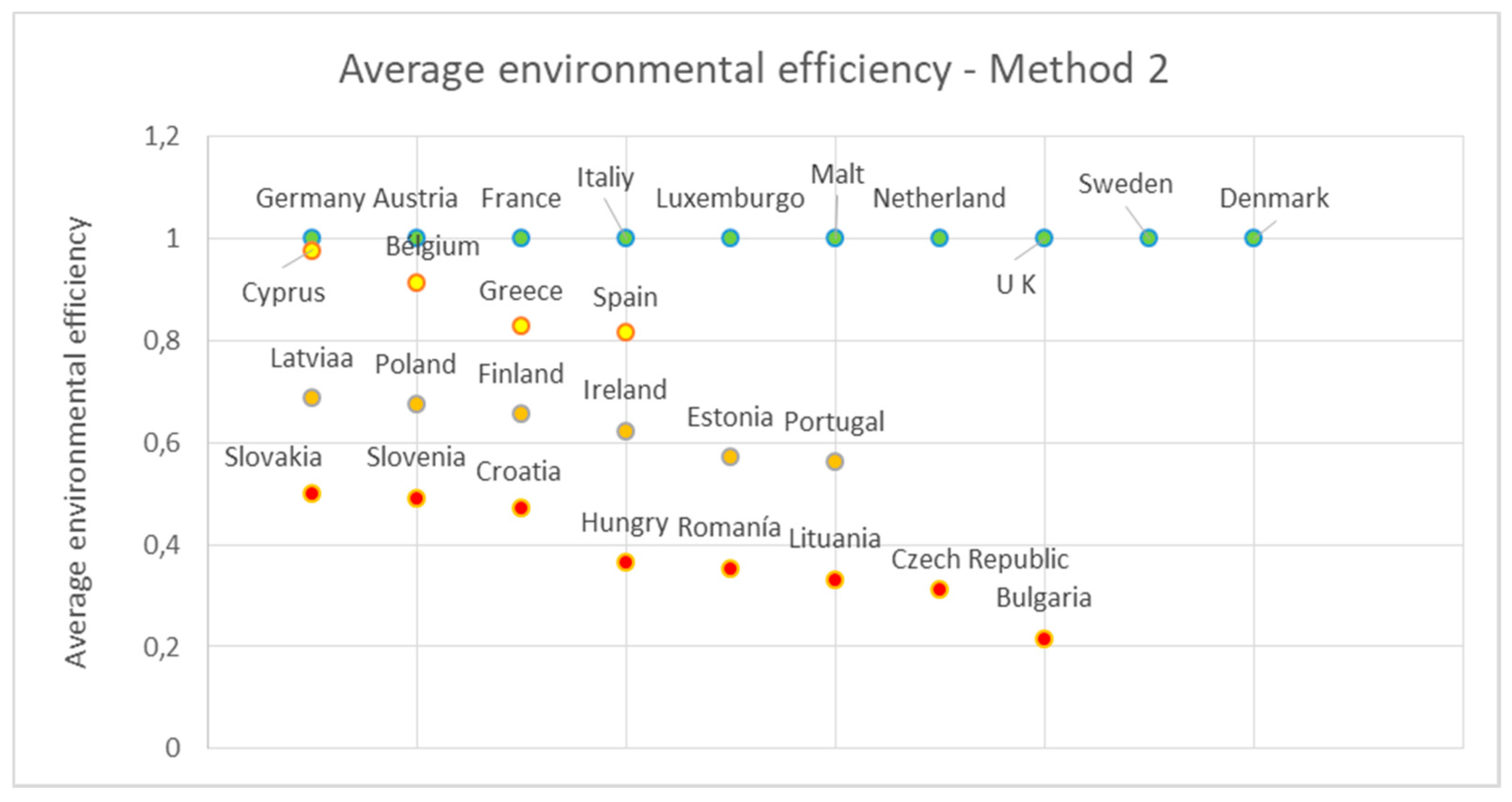
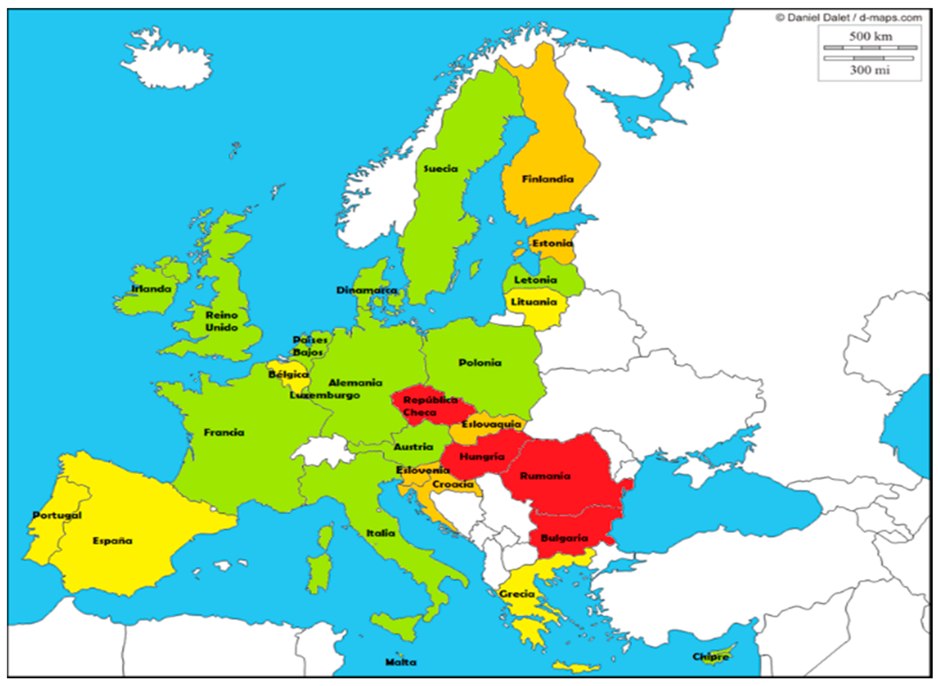
4.3. Establishment of Categories Based on Relative Environmental Efficiency Values

In view of the values of average environmental efficiency, four categories were established:

• Excellent environmental efficiency: for those countries with an average of between 0.9999 and 1 and which was represented with the green color.
• Good environmental efficiency: for those countries with an average between 0.8 and 0.9999 and that are represented by the color yellow.
• Average environmental efficiency: for those countries with an average between 0.5 and 0.79 and which are represented by the color orange.
• Improved environmental efficiency: for those countries with an average between 0 and 0.49 and which are represented by the color red.

Taking into account the average relative environmental efficiency values obtained with Method 1, the countries are divided into the categories established above. The results are shown in Figure 1.

In this way, according to the data obtained with Method 1, the 28 countries of the European Union are divided into the different categories in the following way:

• 14 countries are in the category “Excellent environmental efficiency” and are Germany, Austria, Cyprus, Denmark, France, Ireland, Italy, Latvia, Luxembourg, Malta, the Netherlands, Poland, the United Kingdom and Sweden.
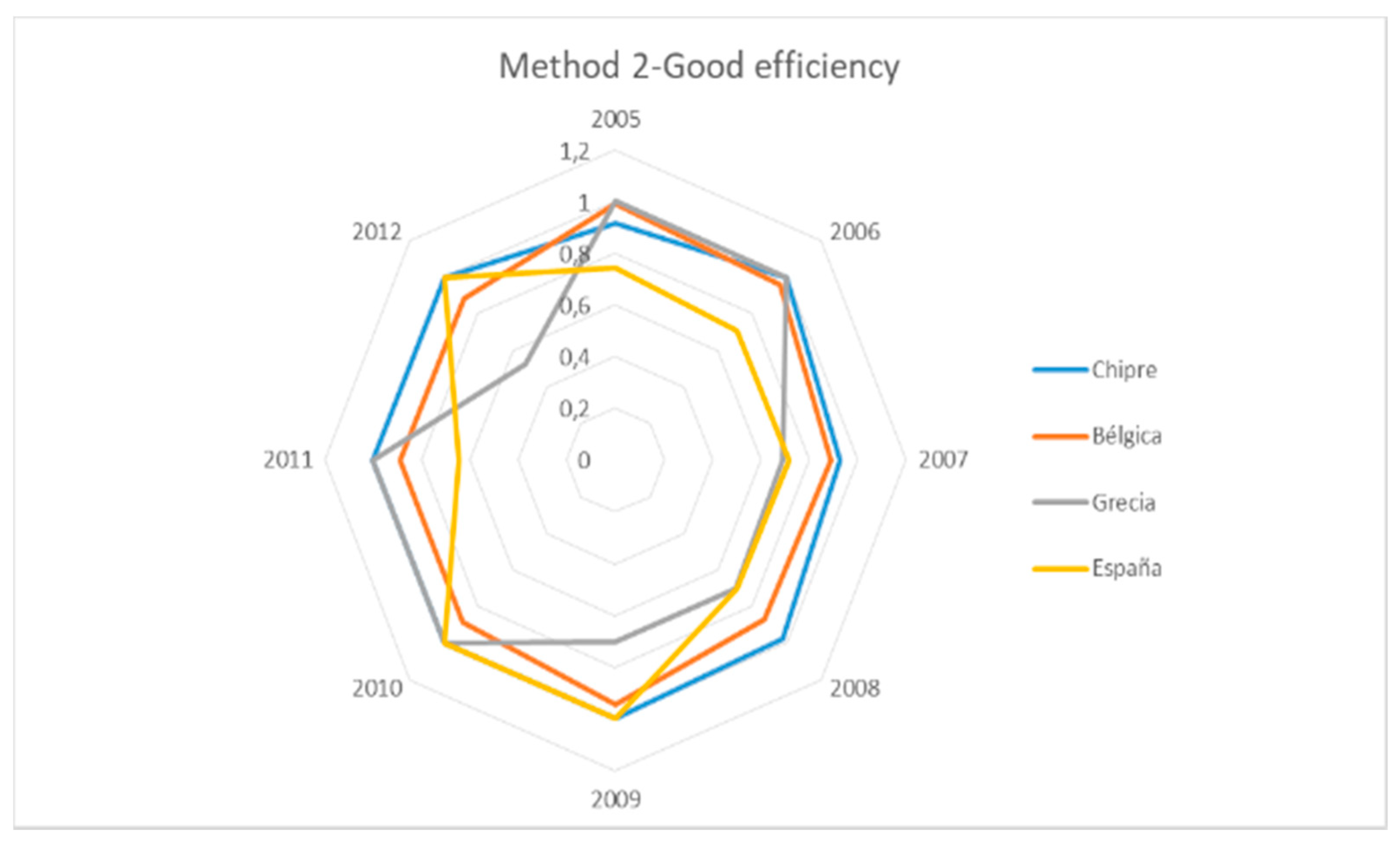
• 5 countries are in the category of “Good environmental efficiency” and are Belgium, Spain, Greece, Lithuania and Portugal.
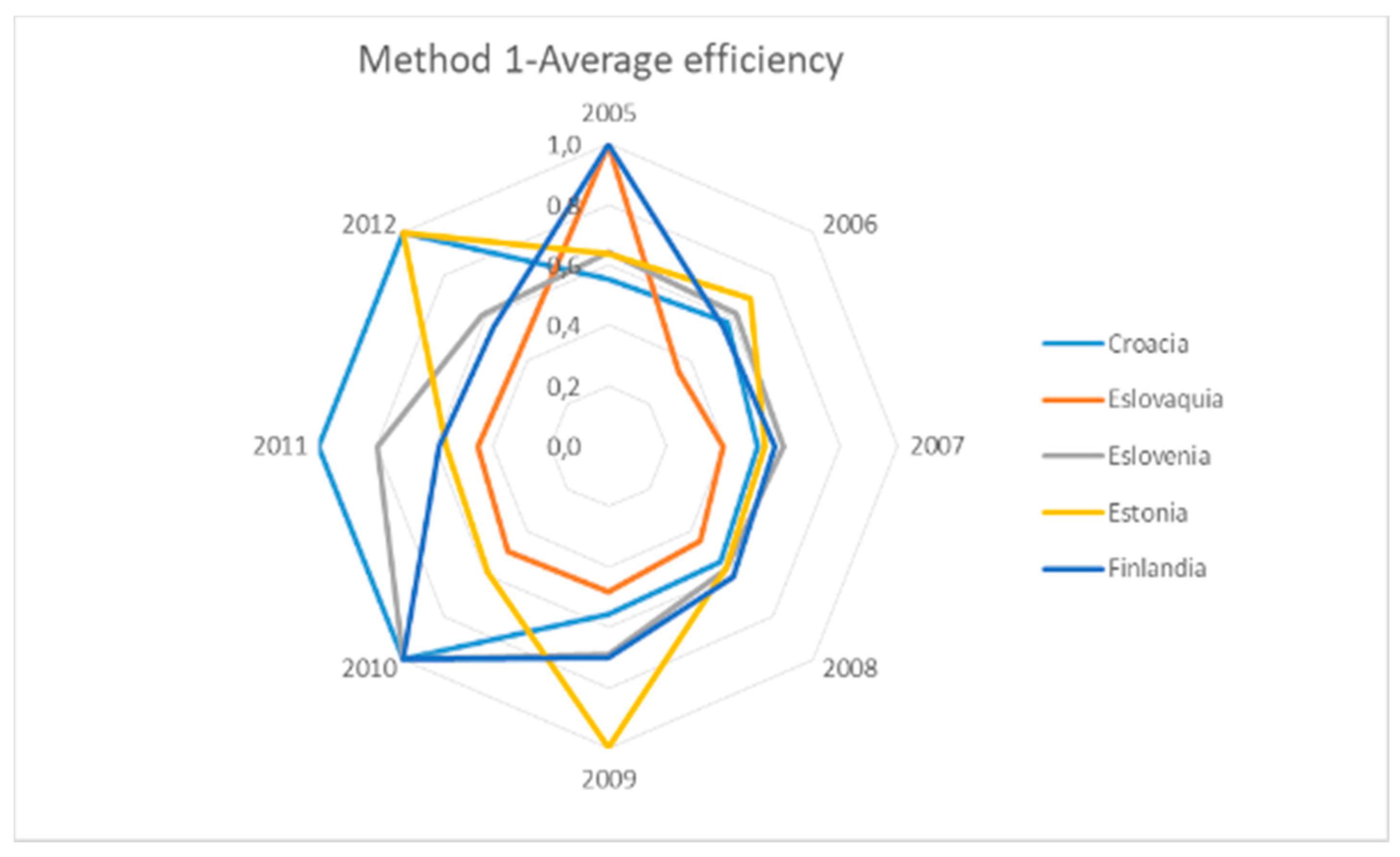
• 5 countries are in the category of “Average environmental efficiency” and are Croatia, Slovakia, Slovenia, Estonia and Finland.
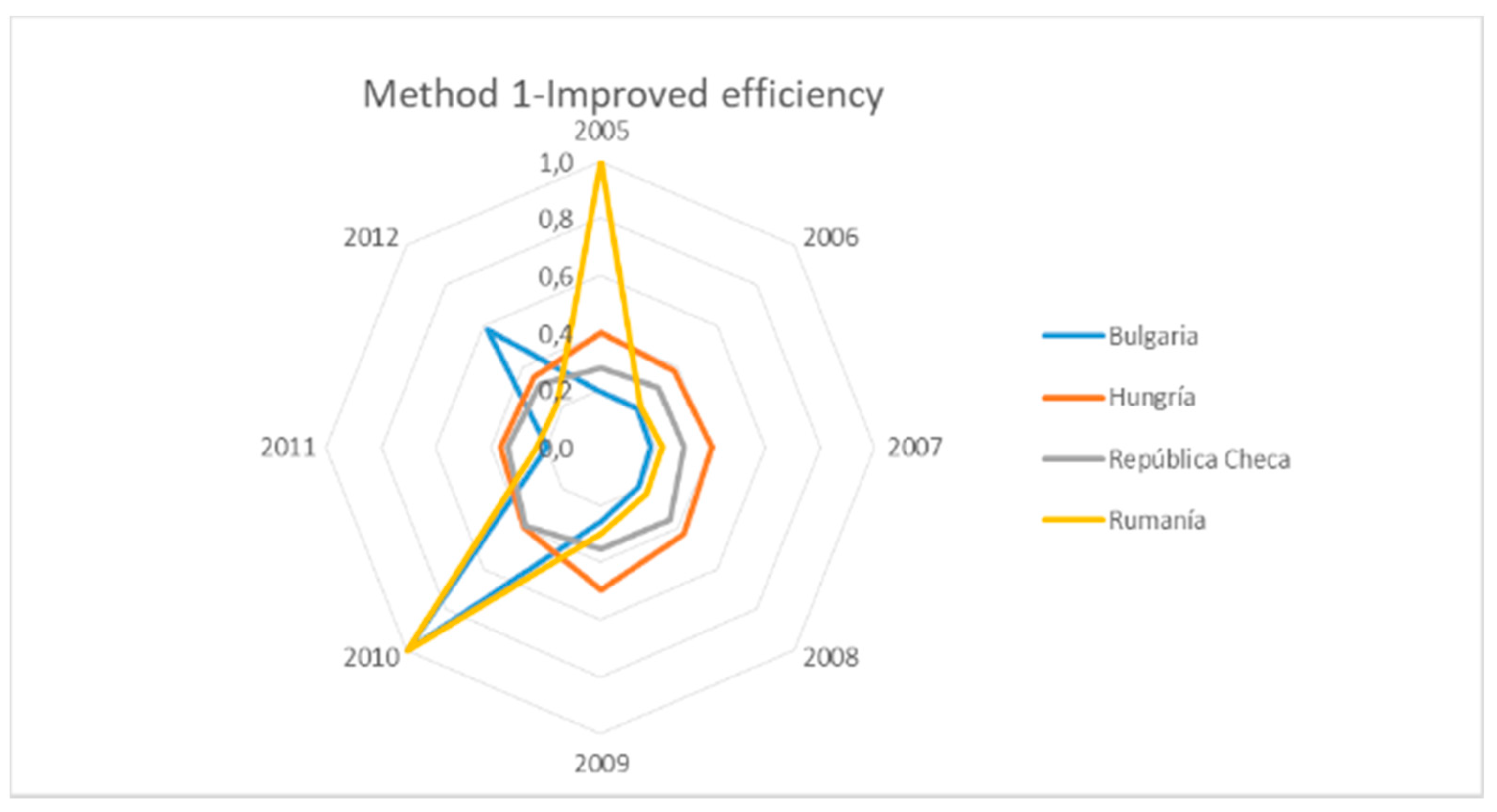
• The remaining 4 countries are in the category of “Improvable environmental efficiency” and are Bulgaria, Hungary, Czech Republic and Romania.

The countries with the highest average environmental efficiency are Germany, Denmark and Austria, while the countries with the lowest average environmental efficiency are Hungary, Bulgaria and the Czech Republic. Figure 2 shows the average environmental efficiency data for the 28 countries obtained with Method 1.

Then, the 28 countries of the European Union were classified by category, but this time according to the data obtained with Method 2. The results are shown in Figure 2.

Figure 2. Average environmental efficiency of the 28 countries obtained with the DEA 2 Method classified by categories. Source: self made.

Figure 2. Average environmental efficiency of the 28 countries obtained with the DEA 2 Method classified by categories. Source: self made.

Comparing data on average environmental efficiencies with the two methods we have countries that are in the same category for the two methods: Spain, France, Italy, Malta, Greece, Austria, Germany, Luxembourg, Belgium, the Netherlands, Denmark, United Kingdom , Sweden, Finland, Estonia, Czech Republic, Hungary, Romania and Bulgaria.

However, there are countries that do change their category:

• Cyprus goes from excellent efficiency to good efficiency.
• Ireland goes from excellent efficiency to good efficiency.
• Latvia goes from excellent efficiency to average efficiency.
• Lithuania goes from good efficiency to improvable efficiency.
• Poland goes from excellent efficiency to average efficiency.
• Slovakia goes from medium efficiency to improvable efficiency.
• Slovenia goes from medium efficiency to improvable efficiency.
• Croatia goes from medium efficiency to improved efficiency.

As we can see also, the number of countries with an efficiency very close to 1, that is, the countries with an excellent environmental efficiency, is reduced, and the number of countries with an improved environmental efficiency increases. However, in the two methods Germany and Austria remain the two countries with the highest environmental efficiency but the last positions vary since, while in Method 1 the country with the worst efficiency is the Czech Republic, in Method 2 It’s Bulgaria.

Table 10. Classification into categories based on average environmental efficiency with Methods 1 and 2 for the 28 countries in the period 2005–2012. Source: self made.

	Method 2		Method 1
Germany	1	Germany	1
Austria	1	Austria	1
France	1	Denmark	1
Italy	1	Netherland	1
Luxemburg	1	France	1
Malt	1	Sweden	1
Netherland	1	UK	1
UK	1	Malt	1
Sweden	1	Ireland	1
Denmark	1	Cyprus	1
Cyprus	0.97715	Poland	1
Bélgium	0.91412	Italy	1
Greece	0.82744	Luxemburg	1
Spain	0.81481	Latvia	1
Letonia	0.68785	Bélgiium	0.95817
Polond	0.67487	Lithuania	0.95425
Finland	0.65601	Greece	0.9428
Ireland	0.62268	Portugal	0.91205
Estonia	0.57147	Spain	0.87356
Portugal	0.56228	Croatia	0.71897
Slovakia	0.49965	Estonia	0.69877
Slovenia	0.49241	Finland	0.6982
Croatia	0.47221	Slovenia	0.69333
Hungry	0.36453	Slovakia	0.50631
Romanía	0.35469	Romanía	0.42727
Lithuania	0.33238	Hungry	0.40165
Czech Republic	0.31162	Bulgaria	0.34892
Bulgaria	0.21638	Czech Republic	0.32869

shows the countries ordered in the different categories according to their average environmental efficiency value for both Method 1 and Method 2.

In order to synthesize all this information, Figure 3 shows a comparison of the average environmental efficiencies for Method 1 and for Method 2.

To better visualize all this information, we proceeded to represent on a map of Europe the different countries with different colors depending on the category that belongs to it according to the average environmental efficiency data obtained with Method 1. This map is presented in the Figure 4.

Looking at the graphical representation of Figure 8 it can be seen that there are several trends: countries with a higher average environmental efficiency are usually found in the central zone of Europe; the countries with the worst average environmental efficiency are in the southeastern part of Europe; and finally, the countries with an average environmental efficiency of the categories of improvable and average environmental efficiency are distributed throughout the territory occupied by the countries of the European Union but are also usually found in the peripheral areas.

In the same way as for Method 1, we proceeded to elaborate the same type of map but with the average environmental efficiency data of Method 2. The data is shown in Figure 5.

The trend is similar to that of Method 1 (the countries with medium and good environmental efficiency are in the periphery and the countries with excellent environmental efficiency are in the central zone) but the number of countries with improved environmental efficiency is increasing. They are found in southeastern Europe.

Figure 5. Representation of the 28 countries with one color according to their environmental efficiency with Method 2. Source: own elaboration.

Figure 5. Representation of the 28 countries with one color according to their environmental efficiency with Method 2. Source: own elaboration.

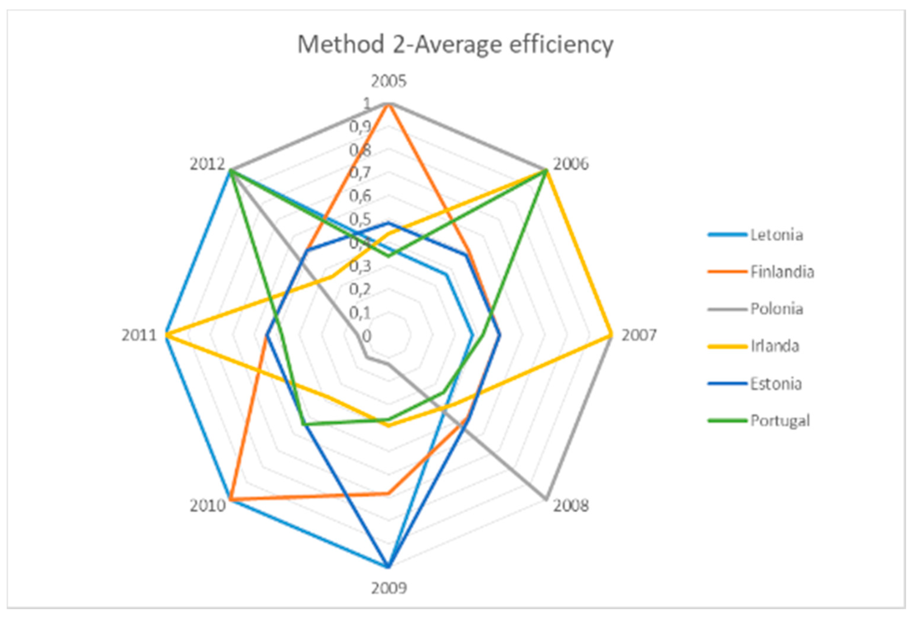
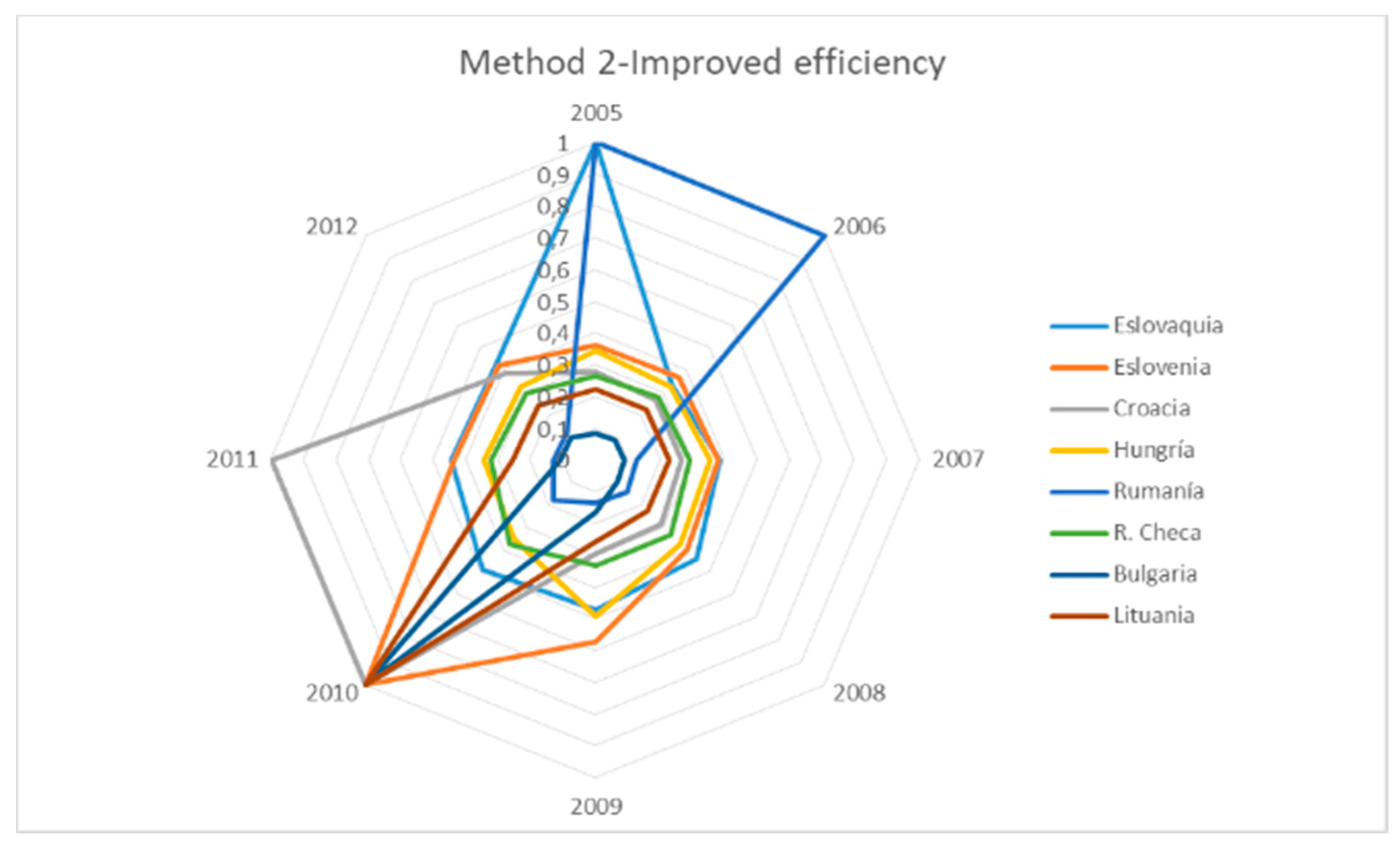
4.4. Evolution of Environmental Efficiency for Different Countries.

Germany has very high efficiency values since both GDP and per capita income remain quite high. However, the emissions also remain quite high, although they do not reach the highest levels observed in the rest of the countries. If Germany had worse economic indicators, it would have a low environmental efficiency because its emissions are not low. A solution for Germany would be to reduce its emissions. It is also observed that almost 50% of the electricity used by Germany comes from coal and that the volume of vehicles is very high. By reducing these two indicators, Germany could reduce its emissions. Another option that Germany could take would be to increase the number of electric vehicles.

• Austria maintains environmental efficiency values very close to 1 because its emissions are not as high as in other countries although the economic indicators are lower than, for example, Germany in the previous case. Despite this, it has environmental efficiency values similar to Germany because its emissions are lower since less than 20% of its electricity comes from coal and oil and its volume of vehicles is not so high. However, the situation could improve if they improve their economic indicators.
• Belgium has a very high environmental efficiency. Their emissions are not very high, which is partly due to the fact that most of the electricity they consume comes from nuclear power plants and less than 20% comes from coal and oil. The number of vehicles is high, although within our study there are countries with a greater volume of vehicles, such as Germany. Its economic indicators are not very high, but as the emissions are not either, a high environmental efficiency is maintained. A possible improvement would come if the GDP and per capita income were improved.
• Bulgaria maintains a low environmental efficiency except in the years 2010 and 2012 in which the environmental efficiency differs a lot from the trend of the other years. Bulgaria shows the lowest environmental efficiency values that have been recorded in our study. This may be due to the fact that GDP and per capita income are very low although emissions are not very high. However, the fact that economic indicators are so low is what makes environmental efficiency very low. It is also true that emissions could be reduced since there is a large volume of vehicles and almost 50% of the electricity comes from coal, although almost the entire remaining part comes from nuclear power plants. The solution for Bulgaria would be to reduce the use of coal to obtain electricity and improve economic indicators.
• Cyprus has environmental efficiency values very close to 1. This is due to the fact that GDP and per capita income are kept at medium values and that emissions are not very high. However, practically 100% of electricity comes from oil, so it would be very convenient to look for other more sustainable sources of energy, such as renewable energies, to improve their situation.
• Croatia maintains an average efficiency but from 2010 its environmental efficiency rises a lot and remains the same in the rest of the years of the study. Croatia shows these relatively low values of environmental efficiency because, although emissions are not too high, GDP and per capita income are not among the highest we find in the countries under study. The volume of vehicles is not excessively high and between the production of electricity from coal and oil do not reach 50% so to improve their situation should improve their economy and perhaps seek other sources of more renewable energy or bet on the nuclear energy that is practically absent in this country. As of 2010, the values of environmental efficiency are very close to 1. This may be due to the fact that the emission values are lower during these years as well as the production of electricity from oil.
• Denmark always shows very high values of environmental efficiency. These values are due to the fact that the emissions have acceptable values, in addition to the fact that the economic indicators are correct, although they are not as high as in Germany, which is the country that shows the best GDP and per capita income among the countries that make up our study. However, the production of electricity from coal is always higher than 34%, so maybe we should look for other sources of energy such as renewables or bet on nuclear energy that is absent in this country.
• Slovakia maintains a low environmental efficiency, except in the year 2005 in which environmental efficiency has a very different value from the trend followed. The emission values are below the average as well as the per capita income, but the GDP is well below the average, which may be the reason why its efficiency values are not too high. It shows values of electricity production from very high nuclear sources (always above 50%) and much higher than those from coal and oil, which is positive from the point of view of reducing emissions. However, to improve its efficiency it should improve its GDP. In addition, environmental measures could be taken such as increasing the number of electric cars, switching to renewable energies, among other measures.
• Slovenia has a greater environmental efficiency in the years 2010 and 2011 However, in the remaining years, environmental efficiency remains at medium values. In 2010 and 2011 the values of the economic indicators are slightly higher than in the rest of the years, this may be the reason why the environmental efficiency is greater in these years, while the CO₂ emissions are also reduced a bit. with respect to previous years. The emission values remain below the average but also the values of the economic indicators, which means that the environmental efficiency is not higher. To improve the situation, it would be necessary to improve its economy. The production of electricity from coal and nuclear sources have similar values around 30%, so the search for other energy sources to try to reduce the use of coal could also be advantageous.
• Spain has a medium-high environmental efficiency but there are three years in which the environmental efficiency is higher and close to 1. Spain has a GDP above the average while in per capita income barely exceeds the average and in most of the cases does not even reach the average. In the emissions, the average values are exceeded. This is what makes the environmental efficiency values are not higher. In the years 2009, 2010 and 2012, the values of carbon dioxide emissions are slightly lower than in the rest of years, which may be the reason why the efficiencies are higher in those years. The solution for Spain would be to improve its per capita income and reduce emissions.
• Estonia maintains an environmental efficiency in average values but there are two years whose values of environmental efficiency go out of the followed trend and they are the year 2009 and the year 2012. Estonia has a GDP and a per capita income well below the average although, despite the fact that 90% of its electricity comes from coal, the emissions are below the average. To achieve greater efficiency, Estonia should improve its economy and bet on other sources of energy to reduce the use of coal, such as renewable energy or perhaps develop nuclear energy that is not exploited in this country.
• Finland has a high environmental efficiency in the years 2005 and 2010. In the rest of the years there are average values of efficiency. The GDP is below the average as well as the emissions but the per capita income does exceed the average. The fact that GDP is relatively low is what can make efficiency no higher. A possible solution for Finland would be to increase its GDP to have greater environmental efficiency in addition to adopting environmental measures that reduce the impact, such as renewable energy.
• France always has a very high environmental efficiency and with few variations, always being very close to 1. The emissions of carbon dioxide and methane are well above the average as well as per capita income and GDP. Although the emissions are relatively high, the GDP is also very high, which makes it have a good efficiency. France should reduce its emissions by reducing the number of vehicles (which is much higher than the average) since it hardly uses coal when most of its electricity comes from nuclear power plants (around 70%).
• In the case of Greece, the values of environmental efficiency are very high for all years except for the last one in which the environmental efficiency decreases a lot. The GDP is below the average as well as the income per capita, but the efficiency is high because the emissions are not high and are well below the average but could be improved if it were achieved to increase the GDP and the rent per capita. The generation of electricity from coal exceeds 50% and if the oil is added already exceeds 70% so that Greece should look for other sources of energy such as renewables. In 2012, the values of economic indicators are lower, which is possibly the reason why efficiency is much lower in that year.
• Hungary shows quite low environmental efficiency values. Unlike many countries, it does not show anomalous environmental efficiency values that go out of the trend that is followed in the rest of years. In Hungary, the economic indicators are below the average which means that, although the emissions are below the average, the values of environmental efficiency are at quite low values. The situation could improve if the country’s economy improved.
• Ireland, like other countries, shows very high values of environmental efficiency that hardly change. In Ireland, GDP is below the average, as opposed to income per capita, but emissions are also below the average, which is what makes their efficiency very high. For the situation to be optimal, Ireland should increase its GDP. Other environmental measures could also be taken to further improve the situation.
• In Italy, the situation is contrary to Ireland. Both countries have a very high environmental efficiency in all years, but while in Ireland it is due to low emissions, in Italy it is because GDP and per capita income are well above the average, but emissions also exceed the average. The advisable thing for Italy would be that they reduced their emissions since the volume of vehicles is very high (in fact it is very above the average).
• In the case of Latvia, efficiency remains very high and without fluctuations in the years of the study. A very positive issue is that very little energy comes from coal and oil or from nuclear sources in Latvia, so perhaps part of their electricity comes from renewable sources, which is very convenient for high environmental efficiency. GDP and per capita income are below the average but emissions are quite low, which makes efficiency high. However, for the situation to be optimal, GDP and per capita income should be increased.
• Lithuania has very high environmental efficiency values. However, in 2007, the value of environmental efficiency is very different from the others and much lower. For emissions, Lithuania shows low values (below the average) which is what possibly makes its efficiency high despite the fact that GDP and per capita income are also low and do not exceed the average. For this reason, Lithuania should improve its economy. In Lithuania little coal and oil are used to obtain electricity, so nuclear energy or renewable sources are mostly used, which is good for high environmental efficiency.
• Luxembourg always shows a very high efficiency. This is because the emissions are quite low and well below the average and also the per capita income is also above the average, but not the GDP. Energy in Luxembourg comes from coal, oil and nuclear sources, so we assume that renewable energies are well developed in this country. The situation could be even better if GDP could be increased.
• Malta maintains a high environmental efficiency during the eight years of study. It has GDP and per capita income values well below the average. However, the emissions are well below the average and are very low, which is what makes their efficiency high. On the other hand, 100% of the energy comes from oil, so to improve its situation one could opt for renewable energies, in addition to improving GDP and per capita income.
• The Netherlands has high and constant environmental efficiency values. Both GDP and per capita income are above average, as are carbon dioxide emissions, although methane emissions are quite low, which means that, together with the good situation of economic indicators, environmental efficiency be high The electricity consumed in Luxembourg does not come from coal, oil or nuclear sources so it can come from renewable sources, which would be very convenient to have a high environmental efficiency. Luxembourg should reduce its CO₂ emissions to make the situation even better.
• Poland presents high environmental efficiency values. The GDP and per capita income values are below the average and CO₂ emissions slightly exceed the average. However, it has methane emission values below the average, which is what can make its efficiency high. On the other hand, 90% of its electricity comes from coal, so it would be necessary to reduce this figure, perhaps with the change to renewable sources of energy. It would also be necessary to reduce CO₂ emissions and increase GDP and per capita income.
• Portugal maintains a high environmental efficiency for all the years of the study except for two years, in 2005 and 2009. Its GDP and per capita income are always below the average and methane emissions are above the average. However, it does present a high efficiency because carbon dioxide emissions are very low and well below the average. Among the electricity that comes from oil and coal, they exceed 50% of the total electricity generation, so it would be advisable to invest in renewable energies, reduce methane emissions and improve GDP and per capita income.
• The United Kingdom shows very high values of environmental efficiency. Its GDP and per capita income values are above the average, in addition to its GDP is quite high, this is what makes its efficiency is high since the emissions are quite high and are above the average, so it would be advisable to reduce these emissions, for example, by reducing the volume of vehicles that is quite high in this country or, better still, replacing conventional vehicles with electric or hybrid vehicles.
• The Czech Republic shows low efficiency values and there is no data other than the trend followed. These values are due to the fact that GDP and per capita income are below the average, although emissions are slightly lower than the average, so it would be better to improve GDP and per capita income and reduce emissions. 60% of the energy comes from coal, so it would also be convenient to increase the energy coming from renewable sources.
• Romania maintains its low environmental efficiency values. However, there are two years in which the environmental efficiency is very different, in 2005 and 2010. In Romania, GDP and per capita income are well below the average and methane emissions are above the average. average, which means that, although carbon dioxide emissions are below the average, environmental efficiency is low. To improve their environmental efficiency, GDP and per capita income should be improved, in addition to reducing methane emissions.
• In the case of Sweden, environmental efficiency is always high. GDP does not exceed the average, although income per capita does, and carbon dioxide and methane emissions are quite low and do not exceed the average. This is what makes its environmental efficiency high but could still be improved if GDP were increased. There is also the fact that there is hardly any electricity produced from oil and coal, which is favorable for high environmental efficiency.
• The variations in the values of environmental efficiency exposed previously are shown in Figure 6, Figure 7, Figure 8 and Figure 9 in which the environmental efficiency values for each country have been represented during the 8 years of the study but grouped in the categories established above.

Figure 6. Variation in environmental efficiency in the years 2005–2012 with the DEA Method 1 and for Method 2 for the 14 countries in the category “Excellent environmental efficiency”. Source: self made.

Figure 6. Variation in environmental efficiency in the years 2005–2012 with the DEA Method 1 and for Method 2 for the 14 countries in the category “Excellent environmental efficiency”. Source: self made.

Figure 7. Variation in environmental efficiency in the years 2005–2012 with the DEA Method 1 and for Method 2 for the 14 countries in the category “Good environmental efficiency”. Source: self made.

Figure 7. Variation in environmental efficiency in the years 2005–2012 with the DEA Method 1 and for Method 2 for the 14 countries in the category “Good environmental efficiency”. Source: self made.

Figure 8. Variation in environmental efficiency in the years 2005–2012 with the DEA Method 1 and for Method 2 for the 14 countries in the category “Average environmental efficiency”. Source: self made.

Figure 8. Variation in environmental efficiency in the years 2005–2012 with the DEA Method 1 and for Method 2 for the 14 countries in the category “Average environmental efficiency”. Source: self made.

Figure 9. Variation in environmental efficiency in the years 2005–2012 with the DEA Method 1 and for Method 2 for the 14 countries in the category “Improved environmental efficiency”. Source: self made.

Figure 9. Variation in environmental efficiency in the years 2005–2012 with the DEA Method 1 and for Method 2 for the 14 countries in the category “Improved environmental efficiency”. Source: self made.

4.5. Temporal Evolution of Average Environmental Efficiency

Regarding the evolution of environmental efficiency for the 8 years of study, (2005–2012, the last years for which data are available for all countries) there are certain countries in which environmental efficiency remains fairly constant and high varying between 0.999999 and 1. These countries usually coincide with the countries that we have included in the category of “excellent environmental efficiency” [42,43].

• There are countries that also maintain a very high environmental efficiency in the 8 years but lower than the countries with excellent environmental efficiency. This would be the case of Belgium, which maintains a high environmental efficiency with slight variations.
• There are countries that follow a trend and their values of environmental efficiency fluctuate little in the eight years of the study. This would be the case, for example, of Hungary and the Czech Republic.
• We also find countries that follow a trend except in some years in which the values of environmental efficiency go out of the trend followed and are much higher than in the remaining years, even reaching an efficiency of 100%. This occurs in countries such as Bulgaria, Spain and Romania, among others (perhaps because they are countries with a more unstable economy and which are more sensitive to changes in the global economic situation) and usually also occur in specific years such as 2005 or 2011 but it is in 2010 that the largest amount of anomalous data is concentrated for the different countries with a large number of them with an efficiency close to 1 when in the remaining years they have a much lower efficiency [44].
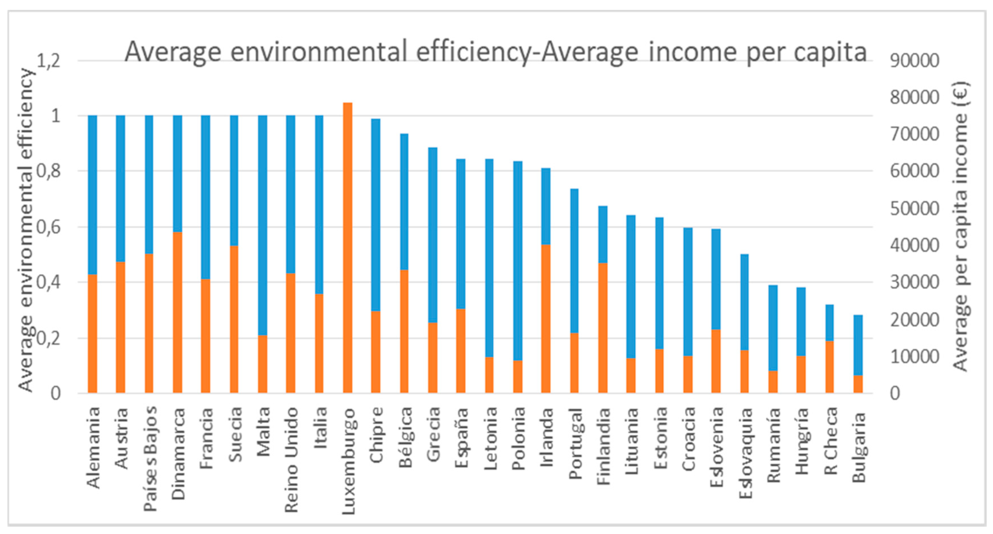
• Subsequently, we obtain the average environmental efficiency data for each of the years of the study, making the average of the environmental efficiency values of all the countries, for both Method 1 and Method 2 and then make the average between Method 1 and Method 2 to analyze the global situation in the Euro Zone. Based on the results obtained for the mean of Methods 1 and 2, it can be seen that in the eight years in which we have done the study, the values of environmental efficiency are quite high, with values that fluctuate between 0.73605 the year in which the average environmental efficiency was lower than it was in 2007 and 0.87039 the year with the highest average environmental efficiency that was 2010. This is due to the fact that in 2010 many countries show a very high environmental efficiency and higher than in the rest of the years due to the fact that in that year the emissions are somewhat lower. We have also obtained an average efficiency value for the total of the European Union from the average of the values we had obtained from the mean of Methods 1 and 2. This value is 0.7824 which is in the category of Average environmental efficiency but it is quite high. All these values are in

  Table 11. Values of average environmental efficiency for the years 2005–2012 obtained with the DEA Method 1 and for Method 2 based on the average environmental efficiency data of the 28 countries of the EU. Average of the values of Methods 1 and 2. Average environmental efficiency value for the total of the European Union. Source: self made.

  	Method 1	Méethod 2	Average	Total Average European Union
  2005	0.86017851	0.74395426	0.80206639	0.78242436
  2006	0.80886046	0.74688476	0.77787261
  2007	0.78810251	0.68400509	0.7360538
  2008	0.81113359	0.6682874	0.7397105
  2009	0.84051984	0.71179776	0.7761588
  2010	0.92367475	0.81711428	0.87039451
  2011	0.83072642	0.72399294	0.77735968
  2012	0.84054784	0.71900935	0.7797786

  [45].

4.6. Obtaining Average Values between Method 1 and Method 2

Once all these evaluations of the data were made, we proceeded to extract average data between Methods 1 and 2. These values are obtained by making the average of the average environmental efficiency values obtained with Method 1 and those obtained with Method 2. The results obtained are shown in

Table 12. Average values of Methods 1 and 2 for the average environmental efficiency of the 28 countries considered in the years 2005–2012. Source: self made.

	Method 1	Method 2	Average
Germany	1	1	1
Austria	1	1	1
Netherland	1	1	1
Denmark	1	1	1
France	1	1	1
Sweden	1	1	1
Malt	1	1	1
UK	1	1	1
Italy	1	1	1
Luxemburg	1	1	1
Cyprus	1	0.977155	0.9885775
Belgium	0.95817106	0.91412867	0.93614987
Greece	0.94280217	0.82744886	0.88512552
Espain	0.87356326	0.81481902	0.84419114
Latvia	1	0.68785791	0.84392896
Poland	1	0.67487704	0.83743852
Ireland	1	0.62268811	0.81134406
Portugal	0.91205631	0.56228108	0.7371687
Finland	0.69820809	0.65601299	0.67711054
Lithuania	0.95425344	0.33238138	0.64331741
Estonia	0.69877384	0.57147078	0.63512231
Croatia	0.71897334	0.47221884	0.59559609
Slovenia	0.69333977	0.49241602	0.5928779
Slovakia	0.50631401	0.49965621	0.50298511
Romanía	0.42737165	0.35469841	0.39103503
Hungry	0.40165806	0.36453795	0.38309801
Czech.Rep	0.32869324	0.31162983	0.32016153
Bulgaria	0.34892545	0.21638236	0.2826539

and in Figure 10.

In view of these results, the countries within the category of excellent environmental efficiency would be Germany, Austria, the Netherlands, Denmark, France, Sweden, Malta, the United Kingdom, Italy, Luxembourg; those in the category of good environmental efficiency would be Cyprus, Belgium, Greece, Spain, Latvia, Poland and Ireland; the countries with average environmental efficiency would be Portugal, Finland, Lithuania, Estonia, Croatia, Slovenia and Slovakia; the countries with improved environmental efficiency would be Romania, Hungary, the Czech Republic and Bulgaria. Germany and Austria remain the countries with the highest average relative environmental efficiency, while Bulgaria and the Czech Republic have the lowest values.

4.7. Improved Analysis Method (MAM)

One issue that is observed by analyzing the average environmental efficiency data of Methods 1 and 2 is that there are many countries that have very different characteristics, are all included in the category of excellent environmental efficiency and have all an environmental efficiency close to 1, for what perhaps the DEA Method is a good tool to divide the countries into different categories according to their relative environmental efficiency but is not able to bias the values. Thus, we have in the same category countries with very different conditions. To discriminate the data, we make the comparison between the average environmental efficiency (obtained from the average of the data of Method 1 and Method 2) of all the countries and the average GDP for the years considered in our study. The data is shown in Figure 11. Average GDP for the 28 countries in the years 2005–2012. Source: self made.

Indeed, we can verify that although there are countries that have a very similar average environmental efficiency, their real situation is not the same as they have many differences in important parameters, such as GDP. This can be seen for example in the case of Germany and Cyprus or Malta, which although have an average environmental efficiency with a value close to 1, their GDP differ greatly, being in the case of Germany much higher than those of Cyprus and Malta, among other countries. Spain, on the other hand, occupies the fifth best GDP among the countries that we are studying, however, regarding environmental efficiency, it occupies the nineteenth position, which supports this affirmation.

Figure 11. Values of average environmental efficiency obtained from the average environmental efficiency data of Method 1 and average environmental efficiency of Method 2. Source: own calculations.

Figure 11. Values of average environmental efficiency obtained from the average environmental efficiency data of Method 1 and average environmental efficiency of Method 2. Source: own calculations.

Our proposed method (MAM) is to assess the average environmental efficiency obtained with Methods 1 and 2 with respect to the desirable and undesirable outputs and establish the most precise hierarchical order within the countries of the same category.

Thus, we compare again the average environmental efficiency of each country with the average per capita income, the average CO₂ emissions and the average CH₄ emissions for the years 2005–2012 and for each country and we obtain similar results comparing the environmental efficiency with the GDP. The results are shown in Figure 12, Figure 13 and Figure 14.

Then we obtain the relation between the average GDP and the average CO₂ emissions and we see that they are positively related. The countries that show the highest values of GDP and CO₂ are Germany, France and the United Kingdom, which, although they have high CO₂ emissions, also have high GDP, which are the countries that we have obtained that have environmental efficiency. With a value of 1 they are really acting more efficiently. In an intermediate position are Spain, Italy and Poland and at the opposite extreme are the rest of the countries. In this last category may be countries that have low CO₂ emissions but then their GDP is also low and therefore have a high environmental efficiency but although the emissions are low the situation is not optimal since they have little industry and their main activity is tourism or similar so they really are less efficient than Germany, for example. The results are shown in Figure 15.

5. Conclusions

The results of our study show that there are many countries that have a high relative environmental efficiency, being these 14 countries of the 28 that are in the European Union and that were the source of our study. Within these 14 countries are the founding countries of the European Union (CEE, 1957) [39] (Germany, France, Italy, Luxembourg and the Netherlands) and others that entered a few years later (Denmark and the United Kingdom that joined in 1973) so that the reason why they have a high environmental efficiency may be that the environmental policies of the European Union are giving favorable results. However, the countries with the lowest efficiency show values of 0.19, being new countries where these environmental policies are not yet having positive results.

Most countries follow a trend in values of environmental efficiency and the data remains close and high but there are countries that have in some years values of environmental efficiency higher and different from the rest of values. These anomalous values are usually found in the years 2005, 2011, 2012, but it is in 2010 that the highest number of countries with higher than normal values are found.

The overall environmental efficiency value for the European Union as a whole would be 0.78, which is a fairly high value and which falls within the category of average environmental efficiency. However, each country can still improve its situation to increase that value.

In view of the results obtained and the values of the indicators used, three types of solutions have been proposed, with countries needing to apply several of these alternatives for environmental improvement. These alternatives would be:

• Change to more sustainable economic models (such as the Circular Economy) to try to increase its GDP and per capita income: it would be applicable to all countries in general, although in particular to Austria, Belgium, Bulgaria, Croatia, Slovakia, Slovenia, Spain , Estonia, Greece, Hungary, Ireland, Latvia, Malta, Poland, Portugal, Czech Republic, Romania and Sweden. However, it must be pointed out that this solution is complicated to apply and depends more on economic policies.
• Reduce your carbon dioxide or methane emissions or both: Germany, Bulgaria, Spain, France, Italy, the Netherlands, Poland, Portugal, the United Kingdom, the Czech Republic and Romania. This could be achieved by using energy sources that do not come from coal or petroleum or proposing changes in the energy model of these countries that make them more sustainable and environmentally efficient.
• Increase the amount of energy from renewable sources by reducing the energy dependence derived from highly polluting fossil fuels such as coal and oil: Cyprus, Croatia, Denmark, Slovenia, Estonia, Greece, Malta, Poland, Portugal and the Czech Republic.

As a general rule, the results of environmental efficiency are quite similar in the two methods used in our study, although they are usually lower in Method 2. However, we also find countries where efficiency is much lower when using Method 2 in the case that your methane emissions were very high. This shows us that if we give the same importance to CO₂ and methane, the results are greater than if we give greater importance to methane, therefore, methane emissions are an important component to reach a good environmental efficiency and should be Take measures to reduce methane emissions at the level of the European Union.

The countries that really have a very high environmental efficiency are Germany, France and the United Kingdom that are those that present high CO₂ emissions but keeping GDP and income per capita also high, these countries being the ones that most comply with the objectives of the Union European Union “to promote sustainable development based on balanced economic growth and the protection of the environment”.

In general, we observed that the DEA methods that have been used to measure eco-efficiency or environmental efficiency are quite accurate and are a good tool applied to categorize situations. However, it is necessary to improve these methods with the introduction of a more rigorous analysis through the implementation of new methods of assessment such as the one proposed (MAM) in our study and to allow hierarchical situations within each resulting category. What can leave the doors open to future studies oriented in this line.

References

- Hansen, J.; Sato, M.; Kharecha, P.; Russell, G.; Lea, D.W.; Siddall, M. Climate change and trace gases. Philos. Trans. R. Soc. Eng. Sci. 2007, 365, 1925–1954. [Google Scholar] [CrossRef] [PubMed]
- Harlem-Brundtland, G. Our Common Future. Brundtland Commission on Environment Development Report. 1987. Available online: http://www.ecominga.uqam.ca/PDF/BIBLIOGRAPHIE/GUIDE_LECTURE_1/CMMAD-Informe-Comision-Brundtland-sobre-Medio-Ambiente-Desarrollo.pdf (accessed on 1 June 2019).
- United Nations Conference on Environment and Development. Rio Declaration on Environment and Development. 1992. Available online: http://www.unesco.org/education/pdf/RIO_S.PDF (accessed on 1 June 2019).
- United Nations Framework Convention on Climate Change (UNFCCC). Kyoto Protocol. 1997. Available online: https://unfccc.int/resource/docs/convkp/kpspan.pdf (accessed on 1 June 2019).
- United Nations Framework Convention on Climate Change (UNFCCC). Adoption of the Paris Agreement. 2015. Available online: https://unfccc.int/resource/docs/2015/cop21/spa/l09s.pdf (accessed on 1 June 2019).
- World Business Council for Sustainable Development (WBCSD). Eco-Efficiency. 1992. Available online: https://www.sciencedirect.com/topics/engineering/world-business-council-for-sustainable-development (accessed on 1 June 2019).
- Unión Europea (UE). Paquete de Medidas Sobre Clima y Energía Hasta 2020. 2007. Available online: https://ec.europa.eu/clima/policies/strategies/2020_es (accessed on 1 June 2019).
- Lundgren, T.; Zhou, W.C. Firm performance and the role of environmental management. J. Environ. Manag. 2017, 203, 330–341. [Google Scholar] [CrossRef] [PubMed]
- Charnes, A.; Cooper, W.W.; Rhodes, E. Measuring the efficiency of decisión making units. Eur. J. Oper. Res. 1978, 2, 429–444. [Google Scholar] [CrossRef]
- Cook, W.D.; Seiford, L.M. Data envelopment analysis (DEA)—Thirty years on. Elsevier. Eur. J. Oper. Res. 2009, 192, 1–17. [Google Scholar] [CrossRef]
- Cook, W.D.; Zhu, J. Data Envelopment Analysis: Modeling Operational Processes and Measuring Productivity; 2008; ISBN-10: 1434830233. [Google Scholar]
- Charnes, A.; Cooper, W.W.; Golany, B.; Seiford, L.; Stutz, J. Foundations of data envelopment analysis and Pareto-Koopmans empirical production functions. J. Econ. 1985, 30, 91–107. [Google Scholar] [CrossRef]
- Banker, R.D.; Charnes, A.; Cooper, W.W. Some models for estimating technical and scale inefficiencies in data development analysis. Manag. Sci. 1984, 30, 1078–1092. [Google Scholar] [CrossRef]
- Green, R.H.; Cook, W.; Doyle, J. A note on the additive data envelopment analysis model. J. Oper. Res. Soc. 1997, 48, 446–448. [Google Scholar] [CrossRef]
- Fare, R.; Lovell, C. Measuring the technical efficiency of production. J. Econ. Theory 1978, 19, 150–162. [Google Scholar] [CrossRef]
- Fare, R.; Lovell, C. Measuring the technical efficiency of production-Reply. J. Econ. Theory 1981, 25, 453–454. [Google Scholar] [CrossRef]
- Pastor, J.T.; Ruiz, J.l.; Sirvent, I. An enhanced DEA Russel graph efficiency measure. Eur. J. Oper. Res. 1999, 115, 596–607. [Google Scholar] [CrossRef]
- Cooper, W.W.; Park, K.S.; Yu, G. IDEA and AR-IDEA: Models for dealing with imprecise data in DEA. Manag. Sci. 1999, 45, 597–607. [Google Scholar] [CrossRef]
- De Clercq, D.; Wen, Z.; Caicedo Luis Caicedo, L.; Cao, X.; Fan, F.; Xu, R.F. Application of DEA and statistical inference to model the determinants of biomethane production efficiency: A case study in south China. Appl. Energy 2017, 205, 1231–1243. [Google Scholar] [CrossRef]
- Chen, W.; Zhou, K.L.; Yang, S.L. Evaluation of China’s electric energy efficiency under environmental constraints: A DEA cross efficiency model based on game relationship. J. Clean. Prod. 2017, 164, 38–44. [Google Scholar] [CrossRef]
- Zhang, B.; Lu, D.; He, Y.; Chiu, Y.H. The efficiencies of resource-saving and environment: A case study based on Chinese cities. Energy 2018, 150, 493–507. [Google Scholar] [CrossRef]
- Lee, P.; Park, Y.J. Eco-Efficiency Evaluation Considering Environmental Stringency. Sustainability 2017, 9, 661. [Google Scholar] [CrossRef]
- Yu, S.H.; Gao, Y.; Shiue, Y.C. A Comprehensive Evaluation of Sustainable Development Ability and Pathway for Major Cities in China. Sustainability 2017, 9, 1483. [Google Scholar] [CrossRef]
- Mardani, A.; Streimikiene, D.; Balezentis, T.; Saman, M.Z.M.; Nor, K.M.; Khoshnava, S.M. Data Envelopment Analysis in Energy and Environmental Economics: An Overview of the State-of-the-Art and Recent Development Trends. Energies 2018, 11, 2002. [Google Scholar] [CrossRef]
- Wu, X.H.; Tan, L.; Guo, J.; Wang, Y.Y.; Liu, H.; Zhu, W.W. A study of allocative efficiency of PM2.5 emission rights based on a zero sum gains data envelopment model. J. Clean. Prod. 2015, 113, 1024–1031. [Google Scholar] [CrossRef]
- Feng, C.; Wang, M. Analysis of energy efficiency and energy savings potential in China’s provincial industrial sectors. J. Clean. Prod. 2017, 164, 1531–1541. [Google Scholar] [CrossRef]
- National Statistics Institute of Spain (INE). 2018. Available online: http://www.ine.es/ (accessed on 1 June 2019).
- National Statistics Institute of Germany (Statistisches Bundesamt). 2018. Available online: https://www.destatis.de/DE/Startseite.html (accessed on 1 June 2019).
- National Institute of Statistics Statistics of France (INSEE). 2018. Available online: https://www.insee.fr/fr/statistiques (accessed on 1 June 2019).
- European Statistical Office (Eurostat, the Statistical Office of the European Communities). 2018. Available online: https://ec.europa.eu/eurostat/publications/statistical-reports (accessed on 1 June 2019).
- International Monetary Fund (IMF). 2018. Available online: http://www.imf.org/en/publications (accessed on 1 June 2019).
- World Bank. 2018. Available online: https://datos.bancomundial.org/indicador (accessed on 1 June 2019).
- World Trade Organization. 2018. Available online: https://www.wto.org/english/res_e/statis_e/statis_e.htm (accessed on 1 June 2019).
- European Central Bank (ECB). 2018. Available online: https://www.ecb.europa.eu/stats/html/index.en.html (accessed on 1 June 2019).
- Bank of Spain. 2018. Available online: https://www.bde.es/bde/es/areas/estadis/ (accessed on 1 June 2019).
- Institute National Statistical Office of Italy (Istat, L’Istituto nazionale di statistica). 2018. Available online: https://www4.istat.it/it/istituto-nazionale-di-statistica (accessed on 1 June 2019).
- Central Bank of England (Bank of England). 2018. Available online: https://www.bankofengland.co.uk/news/statistics (accessed on 1 June 2019).
- Tyteca, D. Linear programming models for the measurement of environmental performance of firms-Concepts and empirical results. J. Product. Anal. 1997, 8, 183–197. [Google Scholar] [CrossRef]
- European Economic Community. Tratado Constitutivo de la Comunidad Económica Europea. 1957. Available online: https://eur-lex.europa.eu/legal-content/ES/TXT/HTML/?uri=CELEX:11957E&from=ES (accessed on 1 June 2019).
- Claver, E.; Molina, J.F.; Tari, J.J. Quality Management and Environmental Management; Editorial Pirámide: Madrid, Spain, 2011; ISBN 978-84-368-2458-2. [Google Scholar]
- Wen, M.L.; Zhang, Q.Y.; Kang, R.; Yang, Y. Some new ranking criteria in data envelopment analysis under uncertain environment. Comput. Ind. Eng. 2017, 110, 498–504. [Google Scholar] [CrossRef]
- Yang, J.; Li, X.G.; Zhou, Z.X. A Cross-efficiency data envelopment analysis (DEA) based model for measuring environmental performance. Environ. Eng. Manag. J. 2014, 13, 1139–1146. [Google Scholar]
- Zhou, P.; Poh, K.L.; Ang, B.W. Data Envelopment Analysis for Measuring Environmental Performance. In Handbook of Operations Analytics Using Data Envelopment Analysis; Springer: Boston, MA, USA, 2016; pp. 31–49. [Google Scholar]
- European Union. A Healthy and Sustainable Environment for Generations to Come. 2014. Available online: https://publications.europa.eu/es/publication-detail/-/publication/3456359b-4cb4-4a6e-9586-6b9846931463 (accessed on 1 June 2019).
- Gen, Z.Q.; Dong, J.G.; Han, Y.M.; Zhu, Q.X. Energy and environment efficiency analysis based on an improved environment DEA cross-model: Case study of complex chemical processes. Appl. Energy 2017, 205, 465–476. [Google Scholar] [CrossRef]