Gaussian Processes for Data Fulfilling Linear Differential Equations  ^†

Abstract

A method to reconstruct fields, source strengths and physical parameters based on Gaussian process regression is presented for the case where data are known to fulfill a given linear differential equation with localized sources. The approach is applicable to a wide range of data from physical measurements and numerical simulations. It is based on the well-known invariance of the Gaussian under linear operators, in particular differentiation. Instead of using a generic covariance function to represent data from an unknown field, the space of possible covariance functions is restricted to allow only Gaussian random fields that fulfill the homogeneous differential equation. The resulting tailored kernel functions lead to more reliable regression compared to using a generic kernel and makes some hyperparameters directly interpretable. For differential equations representing laws of physics such a choice limits realizations of random fields to physically possible solutions. Source terms are added by superposition and their strength estimated in a probabilistic fashion, together with possibly unknown hyperparameters with physical meaning in the differential operator.

1. Introduction

The larger context of the present work is the goal to construct reduced complexity models as emulators or surrogates that retain mathematical and physical properties of the underlying system. Similar to usual numerical models, such methods aim to represent infinite systems by exploiting finite information in some optimal sense. In the spirit of structure preserving numerics the aim here is to move errors to the “right place”, in order to retain laws such as conservation of mass, energy or momentum.

This article deals with Gaussian process (GP) regression on data with additional information known in the form of linear, generally partial differential equations (PDEs). An illustrative application is the reconstruction of an acoustic sound pressure field and its sources from discrete microphone measurements. GPs, a special class of random fields, are used in a probabilistic rather than a stochastic sense: approximate a fixed but unknown field from possibly noisy local measurements. Uncertainties in this reconstruction are modeled by a normal distribution. For the limit of zero measured data a prior has to be chosen whose realizations take values in the expected order of magnitude. An appropriate choice of a covariance function or kernel guarantees that all fields drawn from the GP at any stage fulfill the underlying PDE. This may require to give up stationarity of the process.

Techniques to fit GPs to data from PDEs has been known for some time, especially in the field of geostatistics [1]. A general analysis including a number of important properties is given by [2]. In these earlier works GPs are usually referred to as Kriging and stationary covariance functions/kernels as covariograms. A number of more recent works from various fields [3,4,5] use the linear operator of the problem to obtain a new kernel function for the source field by applying it twice to a generic, usually squared exponential, kernel. In contrast to the present approach, that method is suited best for source fields that are non-vanishing across the whole domain. In terms of deterministic numerical methods one could say that the approach correspond to meshless variants of the finite element method (FEM). The approach in the present work instead represents a probabilistic variant of a procedure related to the boundary element method (BEM), also known as the method of fundamental solutions (MFS) or regularized BEM [6,7,8]. As in the BEM, the MFS also builds on fundamental solutions, but allows to place sources outside the boundary rather than localizing them on a layer. Thus the MFS avoids singularities in boundary integrals of the BEM while retaining a similar ratio of numerical effort and accuracy for smooth solutions. To the author’s knowledge the probabilistic variant of the MFS via GPs has first been introduced by [9] to solve the boundary value problem of the Laplace equation and dubbed Bayesian boundary elements estimation method ((BE)${}^2$M). This work also provides a detailed treatment of kernels for the 2D Laplace equation. A more extensive and general treatment of the Bayesian context as well as kernels and their connection to fundamental solutions is available in [10] under the term probabilistic meshless methods (PMM).

While Mendes et al. [9] is focused on boundary data of a single homogeneous equation, and Cockayne et al. [10] provides a detailed mathematical foundation, the present work aims to explore the topic further for application and extend the recent work in [11]. Starting from general notions some regression techniques are introduced with emphasis on the role of localized sources. For this purpose Poisson, Helmholtz and heat equation are considered and several kernels are derived and tested. To fit a GP to a homogeneous (source-free) PDE, kernels are built via according fundamental solutions. Possible singularities (sources) are moved outside the domain of interest. In particular, boundary conditions on a finite domain can be either supplied or reconstructed in this fashion. In addition contributions by internal sources are superimposed, using again fundamental solutions in the free field. For that part boundary conditions of the actual problem are irrelevant. The specific approach taken here is most efficient for source-free regions with possibly few localized sources that are represented by monopoles or dipoles.

2. GP Regression for Data from Linear PDEs

Gaussian processes (GPs) are a useful tool to represent and update incomplete information on scalar fields (The more general case of complex valued fields and vector fields is left open for future investigations in this context.) $u\left(\mathbf{x}\right)$, i.e., a real number u depending on a (multi-dimensional) independent variable $\mathbf{x}$. A GP with mean $m\left(\mathbf{x}\right)$ and covariance function of kernel $k(\mathbf{x},{\mathbf{x}}^{\prime })$ is denoted as

$$u\left(\mathbf{x}\right)\sim \mathcal{G}(m\left(\mathbf{x}\right),k(\mathbf{x},{\mathbf{x}}^{\prime })).$$

(1)

The choice of an appropriate kernel $k(\mathbf{x},{\mathbf{x}}^{\prime })$ restricts realizations of (1) to respect regularity properties of $u\left(\mathbf{x}\right)$ such as continuity or characteristic length scales. Often regularity of u does not appear by chance, but rather reflects an underlying law. We are going to exploit such laws in the construction and application of Gaussian processes describing u for the case described by linear (partial) differential equations

$$\widehat{L}u\left(\mathbf{x}\right)=q\left(\mathbf{x}\right).$$

(2)

Here $\widehat{L}$ is a linear differential operator, and $q\left(\mathbf{x}\right)$ is an inhomogeneous source term. In physical laws dimensions of $\mathbf{x}$ usually consist of space and/or time. Physical scalar fields u include e.g. pressure p, temperature T or the electrostatic potential ${\varphi }_{\mathrm{e}}$. Corresponding laws under certain conditions include Gauss’ law of electrostatics for ${\varphi }_{\mathrm{e}}$ with Laplacian $\widehat{L}=\epsilon \Delta$, frequency-domain acoustics for p with Helmholtz operator $\widehat{L}=\Delta -k_0^2$ or thermodynamics for T with heat/diffusion operator $\widehat{L}=\frac{\partial }{\partial t}-D\Delta$. These operators contain free parameters, namely permeability $\epsilon$, wavenumber $k_0$, and diffusivity D, respectively. While $\epsilon$ may be absorbed inside q in a uniform material model of electrostatics, estimation of parameters $k_0$ or D is useful for material characterization.

For the representation of PDE solutions the weight-space view of Gaussian process regression is useful. There the kernel k is represented via a tuple $\mathit{\varphi }\left(\mathbf{x}\right)=({\varphi }_1\left(\mathbf{x}\right),{\varphi }_2\left(\mathbf{x}\right),\cdots )$ of basis functions ${\varphi }_i\left(\mathbf{x}\right)$ that underlie a linear regression model

$$u\left(\mathbf{x}\right)=\mathit{\varphi }{\left(\mathbf{x}\right)}^T\mathbf{w}=\sum _i{\varphi }_i\left(\mathbf{x}\right)w_i.$$

(3)

Bayesian inference starting from a Gaussian prior with covariance matrix ${\Sigma }_{\mathrm{p}}$ for weights $\mathbf{w}$ yields a Mercer kernel

$$k(\mathbf{x},{\mathbf{x}}^{\prime })\equiv {\mathit{\varphi }}^T\left(\mathbf{x}\right){\Sigma }_{\mathrm{p}}\mathit{\varphi }\left({\mathbf{x}}^{\prime }\right)=\sum _{i,j}{\varphi }_i\left(\mathbf{x}\right){\Sigma }_{\mathrm{p}}^{ij}{\varphi }_j\left({\mathbf{x}}^{\prime }\right).$$

(4)

The existence of such a representation is guaranteed by Mercer’s theorem in the context of reproducing kernel Hilbert spaces (RKHS) [8]. More generally one can also define kernels on an uncountably infinite number of basis functions in analogy to (3) via

$$f\left(\mathbf{x}\right)=\widehat{\varphi }\left[w\left(\mathit{\zeta }\right)\right]=〈\varphi (\mathbf{x},\mathit{\zeta }),w\left(\mathit{\zeta }\right)〉=\int \varphi (\mathbf{x},\mathit{\zeta })w\left(\mathit{\zeta }\right)\mathrm{d}\mathit{\zeta },$$

(5)

where $\widehat{\varphi }$ is a linear operator acting on elements $w\left(\mathit{\zeta }\right)$ of an infinite-dimensional weight space parametrized by an auxiliary index variable $\mathit{\zeta }$, that may be multi-dimensional. We represent $\widehat{\varphi }$ via an inner product $〈\varphi (\mathbf{x},\mathit{\zeta }),w\left(\mathit{\zeta }\right)〉$ in the respective function space given by an integral over $\mathit{\zeta }$. The infinite-dimensional analogue to the prior covariance matrix is a prior covariance operator ${\widehat{\Sigma }}_{\mathrm{p}}$ that defines the kernel as a bilinear form

$$k(\mathbf{x},{\mathbf{x}}^{\prime })\equiv 〈\varphi (\mathbf{x},\mathit{\zeta }),{\widehat{\Sigma }}_{\mathrm{p}}\varphi ({\mathbf{x}}^{\prime },{\mathit{\zeta }}^{\prime })〉\equiv \int \varphi (\mathbf{x},\mathit{\zeta }){\Sigma }_{\mathrm{p}}(\mathit{\zeta },{\mathit{\zeta }}^{\prime })\varphi ({\mathbf{x}}^{\prime },{{\zeta }}^{\prime })\mathrm{d}\mathit{\zeta }\mathrm{d}{\mathit{\zeta }}^{\prime }.$$

(6)

Kernels of the form (6) are known as convolution kernels. Such a kernel is at least positive semidefinite, and positive definiteness follows in the case of linearly independent basis functions $\varphi (\mathbf{x},\mathit{\zeta })$ [8].

2.1. Construction of Kernels for PDEs

For treatment of PDEs possible choices of index variables in (4) or (6) include separation constants of analytical solutions, or the frequency variable of an integral transform. In accordance with [10], using basis functions that satisfy the underlying PDE, a probabilistic meshless method (PMM) is constructed. In particular, if $\mathit{\zeta }$ parameterizes positions of sources, and $\varphi (\mathbf{x},\mathit{\zeta })=G(\mathbf{x},\mathit{\zeta })$ in (6) is chosen to be a fundamental solution/Green’s function $G(\mathbf{x},\mathit{\zeta })$ of the PDE, one may call the resulting scheme a probabilistic method of fundamental solutions (pMFS). In [10] sources are placed across the whole computational domain, and the resulting kernel is called natural. Here we will instead place sources in the exterior to fulfill the homogeneous interior problem, as in the classical MFS [6,7,8]. Technically, this is also achieved by setting ${\Sigma }_{\mathrm{p}}(\mathit{\zeta },{\mathit{\zeta }}^{\prime })=0$ for either $\mathit{\zeta }$ or ${\mathit{\zeta }}^{\prime }$ in the interior. For discrete sources localized $\mathit{\zeta }={\mathit{\zeta }}_i$ one obtains again discrete basis functions ${\varphi }_i\left(\mathbf{x}\right)=G(\mathbf{x},{\mathit{\zeta }}_i)$ for (4).

More generally, according to theorem 2 of [2], for linear PDE operators $\widehat{L}$ in (2) with $q\ne 0$ we require a Gaussian process of non-zero mean $m\left(\mathbf{x}\right)$ with

$$\begin{array}{cc}\hfill \widehat{L}m\left(\mathbf{x}\right)& =q\left(\mathbf{x}\right),\hfill \end{array}$$

(7)

$$\begin{array}{cc}\hfill \widehat{L}k(\mathbf{x},{\mathbf{x}}^{\prime })& =0.\hfill \end{array}$$

(8)

Here $\widehat{L}$ acts on the first argument of $k(\mathbf{x},{\mathbf{x}}^{\prime })$. Sources affect only the mean $m\left(\mathbf{x}\right)$ of the Gaussian process, whereas the kernel $k(\mathbf{x},{\mathbf{x}}^{\prime })$ should be based on the homogeneous equation. This hints to the technique of [12] discussed in [13] chapter 2.7 to treat $m\left(\mathbf{x}\right)$ via a linear model added on top of a zero-mean process for the homogeneous equation. In that case we consider is the superposition

$$\begin{array}{cc}\hfill u\left(\mathbf{x}\right)& =u_h\left(\mathbf{x}\right)+u_p\left(\mathbf{x}\right),\hfill \end{array}$$

(9)

$$\begin{array}{cc}\hfill u_h\left(\mathbf{x}\right)& \sim \mathcal{G}(0,k(\mathbf{x},{\mathbf{x}}^{\prime })),\hfill \end{array}$$

(10)

$$\begin{array}{cc}\hfill u_p\left(\mathbf{x}\right)& ={\mathbf{h}}^T\left(\mathbf{x}\right)\mathbf{b},\hfill \end{array}$$

(11)

$$\begin{array}{cc}\hfill \mathbf{b}& \sim \mathcal{N}({\mathbf{b}}_0,B).\hfill \end{array}$$

(12)

where ${\mathbf{h}}^T\left(\mathbf{x}\right)\mathbf{b}$ is a linear model for $m\left(\mathbf{x}\right)$ with Gaussian prior mean ${\mathbf{b}}_0$ and covariance B for the model coefficients. The homogeneous part (10) corresponds to a random process $u_h\left(\mathbf{x}\right)$ where a source-free k is constructed according to (8). The inhomogeneous part (11) may be given by any particular solution $u_p\left(\mathbf{x}\right)$ for arbitrary boundary conditions. Using the limit of a vague prior with ${\mathbf{b}}_0=0$ and $|B^{-1}|\to 0$, i.e., minimum information/infinite prior covariance [12,13], posteriors for mean $\overline{u}$ and covariance matrix $\mathrm{cov}(u,u)$ based on given training data $\mathbf{y}=u\left(X\right)+{\sigma }_{\mathrm{n}}$ with measurement noise variance ${\sigma }_{\mathrm{n}}^2$ are

$$\begin{array}{cc}\hfill \overline{u}\left(X_{★}\right)& =K_{★}^T{K}_y^{-1}(\mathbf{y}-H^T\overline{\mathbf{b}})+H_{★}^T\overline{\mathbf{b}}=K_{★}^T{K}_y^{-1}\mathbf{y}+R^T\overline{\mathbf{b}},\hfill \end{array}$$

(13)

$$\begin{array}{cc}\hfill \mathrm{cov}(u\left(X_{★}\right),u\left(X_{★}\right))& =K_{★★}-K_{★}^T{K}_y^{-1}{K}_{★}+R^T{\left(H{K}_y^{-1}{H}^T\right)}^{-1}R.\hfill \end{array}$$

(14)

Here $X=({\mathbf{x}}_1,{\mathbf{x}}_2,\cdots {\mathbf{x}}_N)$ contains the training points, $X_{★}=({\mathbf{x}}_{★1},{\mathbf{x}}_{★2},\cdots ,{\mathbf{x}}_{★N_{★}})$ the evaluation or test points. Functions of X and $X^{★}$ are to be understood as vectors or matrices resulting from evaluation at different positions, i.e., $\overline{u}\left(X_{★}\right)\equiv (\overline{u}\left({\mathbf{x}}_{★1}\right),\overline{u}\left({\mathbf{x}}_{★2}\right),\cdots ,\overline{u}\left({\mathbf{x}}_{★N_{★}}\right))$ is a tuple of predicted expectation values. The matrix $K\equiv k(X,X)$ is the kernel covariance of the training data with entries $K_{ij}\equiv k({\mathbf{x}}_i,{\mathbf{x}}_j)$ and $\mathrm{cov}{(u\left(X_{★}\right),u\left(X_{★}\right))}_{ij}\equiv \mathrm{cov}(u\left({\mathbf{x}}_{★i}\right),u\left({\mathbf{x}}_{★j}\right))$ are entries of the predicted covariance matrix for u evaluated in the test points ${\mathbf{x}}_{★i}$. Furthermore $K_y\equiv k(X,X)+{\sigma }_{\mathrm{n}}^{2}I$, $K_{★}\equiv k(X,X_{★})$, $K_{★★}\equiv k(X_{★},X_{★})$, $R\equiv H_{★}-H{K}_y^{-1}{K}_{★★}$, and entries of H are $H_{ij}\equiv h_i\left({\mathbf{x}}_j\right)$, $H_{★ij}\equiv h_i\left({\mathbf{x}}_{★j}\right)$, and $\overline{\mathbf{b}}\equiv {\left(H{K}_y^{-1}{H}^T\right)}^{-1}H{K}_y^{-1}\mathbf{y}$.

2.2. Linear Modeling of Sources

A linear model for $m\left(\mathbf{x}\right)$ fulfilling a PDE according to (8) follows directly from the source representation. Consider sources to be modeled as a linear superposition over basis functions

$$q\left(\mathbf{x}\right)=\sum _i{\phi }_i\left(\mathbf{x}\right)q_i$$

(15)

with unknown source strength coefficients $\mathbf{q}=\left(q_i\right)$. To model the mean instead of the source functions themselves, one uses an according superposition

$$m\left(\mathbf{x}\right)=\sum _i{u}_{pi}\left(\mathbf{x}\right)q_i$$

(16)

of particular solutions $u_{pi}\left(\mathbf{x}\right)$ from inhomogeneous equations

$$\widehat{L}{u}_{pi}\left(\mathbf{x}\right)={\phi }_i\left(\mathbf{x}\right).$$

(17)

For the linear Model (9) this means that $\mathbf{b}=\mathbf{q}$ and $h_i\left(\mathbf{x}\right)=u_{pi}\left(\mathbf{x}\right)$. Posterior mean of source strengths and their uncertainty are

$$\begin{array}{cc}\hfill \overline{\mathbf{q}}& ={\left(H{K}_y^{-1}{H}^T\right)}^{-1}H{K}_y^{-1}\mathbf{y},\hfill \end{array}$$

(18)

$$\begin{array}{cc}\hfill \mathrm{cov}(\mathbf{q},\mathbf{q})& ={\left(H{K}_y^{-1}{H}^T\right)}^{-1}.\hfill \end{array}$$

(19)

One can easily check that the predicted mean $\overline{u}\left({\mathbf{x}}_{★}\right)={\overline{u}}_h\left({\mathbf{x}}_{★}\right)+{\overline{u}}_p\left({\mathbf{x}}_{★}\right)$ at a specific point ${\mathbf{x}}_{★}$ in (13) fulfills the linear differential Equation (2). In the homogeneous part ${\overline{u}}_h\left({\mathbf{x}}_{★}\right)=k({\mathbf{x}}_{★},X)K_y^{-1}(\mathbf{y}-H^T\overline{\mathbf{q}})$ sources are absent with $\widehat{L}{\overline{u}}_h\left({\mathbf{x}}_{★}\right)=0$, with $\widehat{L}$ acting on ${\mathbf{x}}^{★}$ here. The particular solution ${\overline{u}}_p\left({\mathbf{x}}_{★}\right)={\mathbf{h}}^T\left({\mathbf{x}}_{★}\right)\overline{\mathbf{q}}={\sum }_i{u}_{pi}\left({\mathbf{x}}_{★}\right){\overline{q}}_i$ adds source contributions $q_i{\phi }_i\left({\mathbf{x}}^{★}\right)$ due to (17). For point monopole sources ${\phi }_i\left(\mathbf{x}\right)=\delta (\mathbf{x}-{\mathbf{x}}_{qi})$ placed at at positions ${\mathbf{x}}_{qi}$, the particular solution $u_{p,i}\left(\mathbf{x}\right)$ equals the fundamental solution $G(\mathbf{x},{\mathbf{x}}_{qi})$ evaluated for the respective source. In the absence of sources the part described in this subsection isn’t modeled and (13) and (14) reduce to posteriors of a GP with prior mean $m\left(\mathbf{x}\right)=0$ where matrix R vanishes.

3. Application Cases

Here the general results described in the previous section are applied to specific equations. Regression is performed based on values measured at a set of sampling points ${\mathbf{x}}_i$ and may also include optimization of hyperparameters $\beta$ appearing as auxiliary variables inside the kernel $k(\mathbf{x},{\mathbf{x}}^{\prime };\beta )$. The optimization step is usually performed in a maximum a posteriori (MAP) sense, choosing ${\beta }_{\mathrm{MAP}}$ as fixed rather than providing a joint probability distribution function including $\beta$ as random variables. We note that depending on the setting this choice may lead to underestimation of uncertainties in the reconstruction of u, in particular for sparse, low-quality measurements.

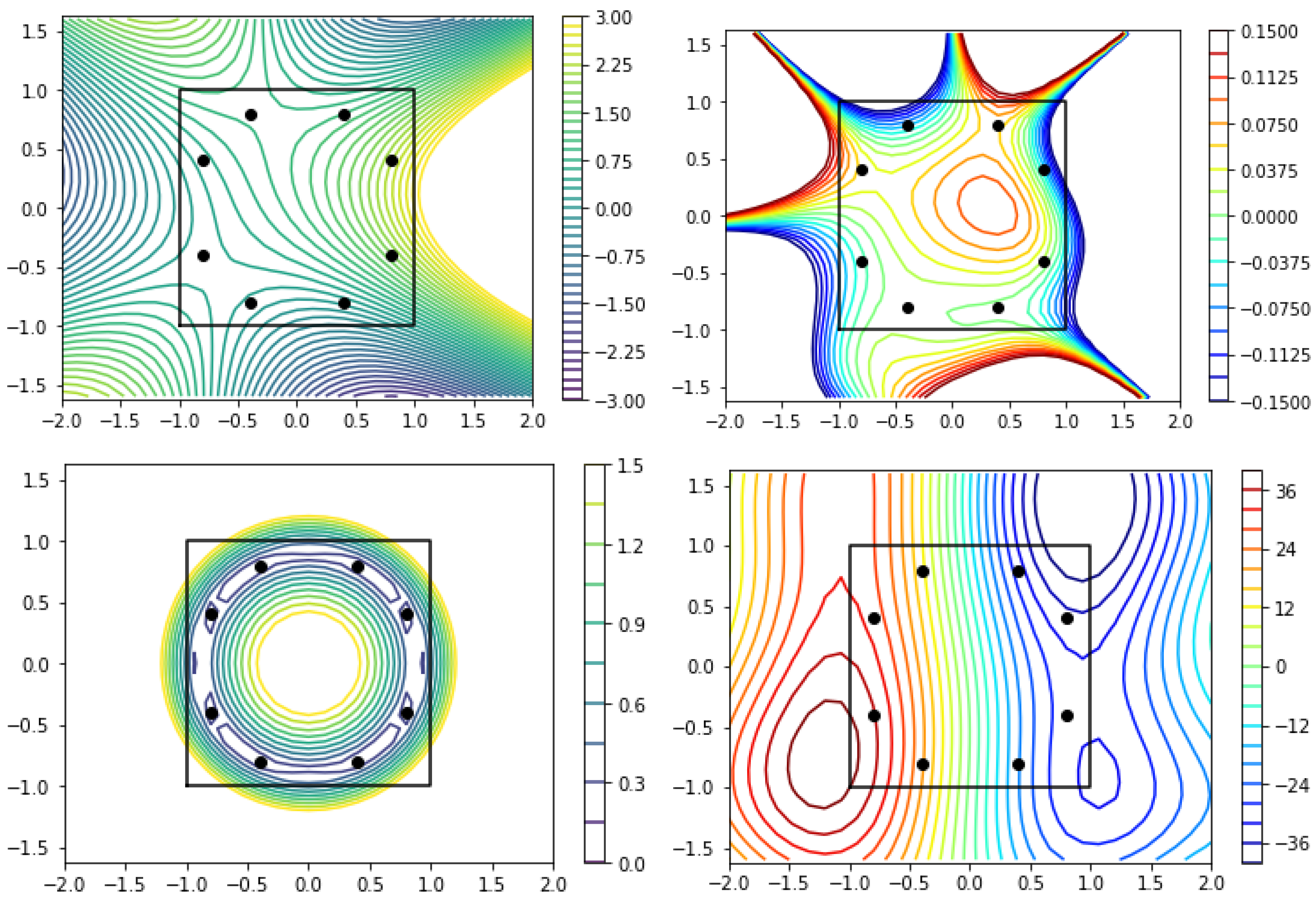
3.1. Laplace’s Equation in Two Dimensions

First we explore construction of kernels in (10) for a purely homogeneous problem in a finite and infinite dimensional index space, depending on the mode of separation. Consider Laplace’s equation

$$\Delta u\left(\mathbf{x}\right)=0.$$

(20)

In contrast to the Helmholtz equation, Laplace’s equation has no scale, i.e., permits all length scales in the solution. In the 2D case using polar coordinates the Laplacian becomes

$$\frac{1}{r}\frac{\partial }{\partial r}\left(r\frac{\partial u}{\partial r}\right)+\frac{1}{r^2}\frac{{\partial }^{2}u}{\partial {\theta }^2}=0.$$

(21)

A well-known family of solutions for this problem based on the separation of variables is

$$u=r^{\pm m}{e}^{\pm im\theta },$$

(22)

leading to a family of solutions

$$r^{m}cos\left(m\theta \right),r^{m}sin\left(m\theta \right),r^{-m}cos\left(m\theta \right),r^{-m}sin\left(m\theta \right).$$

(23)

Since our aim is to work in bounded regions we discard the solutions with negative exponent that diverge at $r=0$. Choosing a diagonal prior that weights sine and cosine terms equivalently [9] and introducing a length scale s as a free parameter we obtain a kernel according to (4) with

$$\begin{array}{cc}\hfill k(\mathbf{x},{\mathbf{x}}^{\prime };s)& =\sum _{m=0}^{\infty }{\left(\frac{r{r}^{\prime }}{s^2}\right)}^m{\sigma }_m^2(cos\left(m\theta \right)cos\left(m{\theta }^{\prime }\right)+sin\left(m\theta \right)sin\left(m{\theta }^{\prime }\right))=\sum _{m=0}^{\infty }{\left(\frac{r{r}^{\prime }}{s^2}\right)}^m{\sigma }_m^{2}cos\left(m(\theta -{\theta }^{\prime })\right).\hfill \end{array}$$

(24)

A flat prior ${\sigma }_m^2=1$ for all polar harmonics and a characteristic length scale s as a hyperparameter, yields

$$\begin{array}{cc}\hfill k(\mathbf{x},{\mathbf{x}}^{\prime };s)& =\frac{1-\frac{r{r}^{\prime }}{s^2}cos(\theta -{\theta }^{\prime })}{1-2\frac{r{r}^{\prime }}{s^2}cos(\theta -{\theta }^{\prime })+\frac{{\left(r{r}^{\prime }\right)}^2}{s^4}}=\frac{1-\frac{\mathbf{x}·{\mathbf{x}}^{\prime }}{s^2}}{1-2\frac{\mathbf{x}·{\mathbf{x}}^{\prime }}{s^2}+\frac{{\left|\mathbf{x}\right|}^2{\left|{\mathbf{x}}^{\prime }\right|}^2}{s^4}}.\hfill \end{array}$$

(25)

This kernel is not stationary, but isotropic around a fixed coordinate origin. Introducing a mirror point ${\overline{\mathbf{x}}}^{\prime }$ with polar angle ${\overline{\theta }}^{\prime }={\theta }^{\prime }$ and radius ${\overline{r}}^{\prime }=s^2/r^{\prime }$ we notice that (25) can be written as

$$k(\mathbf{x},{\mathbf{x}}^{\prime };s)=\frac{{\left|{\overline{\mathbf{x}}}^{\prime }\right|}^2-\mathbf{x}·{\overline{\mathbf{x}}}^{\prime }}{{(\mathbf{x}-{\overline{\mathbf{x}}}^{\prime })}^2},$$

(26)

making a dipole singularity apparent at $\mathbf{x}={\overline{\mathbf{x}}}^{\prime }$. In addition k is normalized to 1 at $\mathbf{x}=0$. Choosing $s>R_0$ larger than the radius $R_0$ of a circle centered in the origin and enclosing the computational domain, we have ${\overline{r}}^{\prime }>s^2/s=s>R_0$. Thus all mirror points and the according singularities are moved outside the domain.

Choosing a slowly decaying ${\sigma }_m^2=1/m$, excluding $m=1$ and adding a constant term yields a logarithmic kernel instead [9] with

$$k(\mathbf{x},{\mathbf{x}}^{\prime };s)=1-\frac{1}{2}ln\left(1-2\frac{\mathbf{x}·{\mathbf{x}}^{\prime }}{s^2}+\frac{{\left|\mathbf{x}\right|}^2{\left|{\mathbf{x}}^{\prime }\right|}^2}{s^4}\right)=1-ln\left(\frac{|\mathbf{x}-{\overline{\mathbf{x}}}^{\prime }|}{\left|{\overline{\mathbf{x}}}^{\prime }\right|}\right).$$

(27)

Instead of a dipole singularity that expression features a monopole singularity at $\mathbf{x}-{\overline{\mathbf{x}}}^{\prime }$ that is avoided as mentioned above.

Using instead Cartesian coordinates $x,y$ to separate the Laplacian provides harmonic functions like

$$u=e^{\pm \kappa x}{e}^{\pm i\kappa y}.$$

(28)

Here all solutions yield finite values at $x=0$, so we don’t have to exclude any of them a priori. Introducing again a diagonal covariance operator in (6) and taking the real part yields

$$\begin{array}{cc}\hfill k(\mathbf{x},{\mathbf{x}}^{\prime })& =\int \phi (\mathbf{x},\kappa ){\sigma }^2\left(\kappa \right)\phi ({\mathbf{x}}^{\prime },\kappa )\mathrm{d}\kappa =\mathrm{Re}{\int }_{-\infty }^{\infty }{\sigma }^2\left(\kappa \right)e^{\kappa (x\pm x^{\prime })}{e}^{i\kappa (y\pm y^{\prime })}\mathrm{d}\kappa .\hfill \end{array}$$

(29)

Setting ${\sigma }^2\left(\kappa \right)\equiv e^{-2{\kappa }^2}$ and choosing a characteristic length scale s together with a possible rotation angle ${\theta }_0$ of the coordinate frame yields the kernel

$$k(\mathbf{x},{\mathbf{x}}^{\prime };s,{\theta }_0)=\frac{1}{2}\mathrm{Re}exp\left(\frac{\left((x+x^{\prime })\pm i(y-y^{\prime })\right){}^2{e}^{i2{\theta }_0})}{s^2}\right).$$

(30)

Other sign combinations do not yield a positive definite kernel – similar to the polar kernel (26) before we couldn’t obtain an fully stationary expression that depends only on differences between coordinates of $\mathbf{x}$ and ${\mathbf{x}}^{\prime }$.

For demonstration purposes we consider an analytical solution to a boundary value problem of Laplace’s equation on a square domain $\Omega$ with corners at $(x,y)=(\pm 1,\pm 1)$. The reference solution is

$$u_{\mathrm{ref}}(x,y)=\frac{1}{2}{e}^{y}cosx+2xcos\left(2y\right)$$

(31)

and depicted in the upper left of Figure 1 together with the extension outside the boundaries. This figure also shows results from a GP fitted based on data with artificial noise of ${\sigma }_{\mathrm{n}}=0.1$ measured at 8 points using kernel (26) with $s=2$. Inside $\Omega$ the solution is represented with errors below $5\%$. This is also reflected in the error predicted by the posterior variance of the GP that remains small in the region enclosed by measurement points. The analogy in classical analysis is the theorem that the solution of a homogeneous elliptic equation is fully determined by boundary values.

In comparison, a reconstruction using a generic squared exponential kernel $k\propto exp({(\mathbf{x}-{\mathbf{x}}^{\prime })}^2/\left(2s^2\right))$ yields a result of similar approximation quality in Figure 2. The posterior covariance of that reconstruction is however not able to capture the vanishing error inside the enclosed domain due to given boundary data. More severely, in contrast to the previous case, the posterior mean $\overline{u}$ doesn’t satisfy Laplace’s equation $\Delta \overline{u}=0$ exactly. This leads to a violation of the classical result that (differences of) solutions of Laplace’s equation may not have extrema inside $\Omega$, showing up in the difference to the reconstruction in Figure 2. This kind of error is quantified by computation of the reconstructed charge density $\overline{q}=\Delta \overline{u}$. This is fine if data from Poisson’s equation $\Delta u=q$ with distributed charges should be fitted instead. However, to keep $\Delta u=0$ exact in $\Omega$, one requires more specialized kernels such as (26).

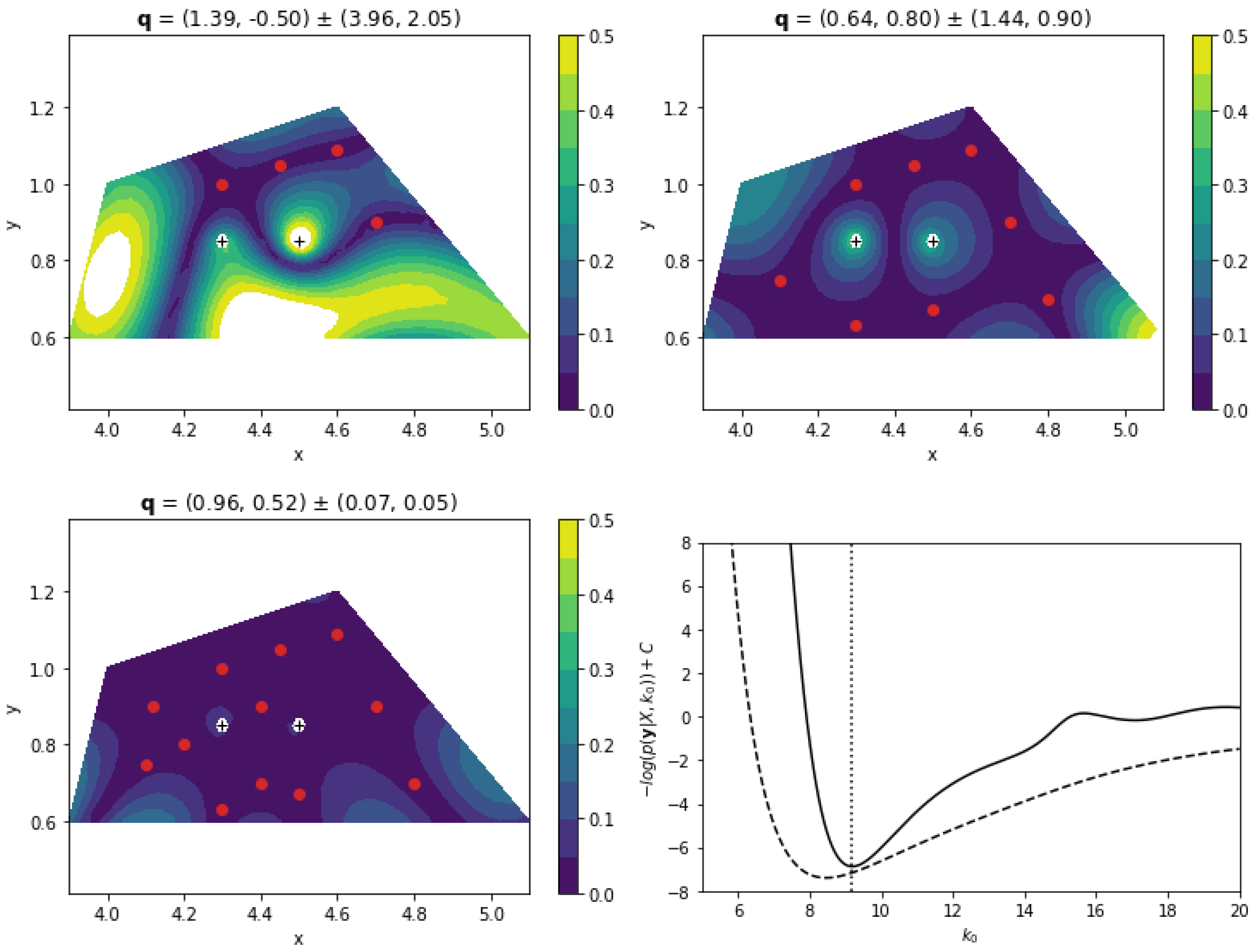
3.2. Helmholtz Equation: Source and Wavenumber Reconstruction

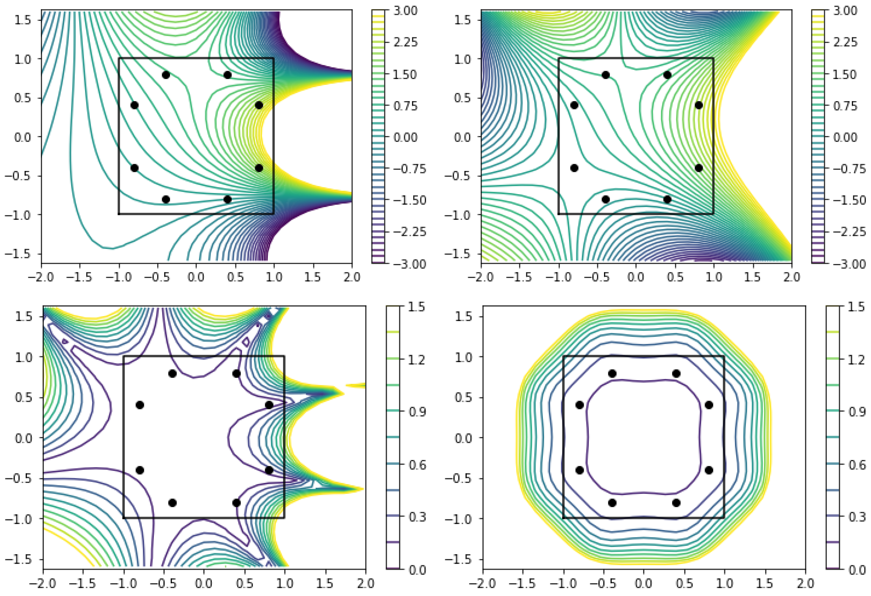
To demonstrate the proposed method in full we now consider the Helmholtz equation with sources

$$\Delta u\left(\mathbf{x}\right)+k_0^{2}u\left(\mathbf{x}\right)=q\left(\mathbf{x}\right).$$

(32)

Stationary kernels based on Bessel functions for the homogeneous equation have been presented in [11]. These functions provide smoothing regularization on the order of the wavelength ${\lambda }_0=2\pi /k_0$ and have been demonstrated to produce excellent field reconstruction from point measurements. Here we consider the two-dimensional case. The method of source strength reconstruction is improved compared to [11], as it constitutes a linear problem according to (18) and (19). Non-linear optimization is instead applied to wavenumber $k_0$ as a free hyperparameter to be estimated during the GP regression.

The setup is the same as in [11]: a 2D cavity with various boundary conditions and two sound sources of strengths 0.5 and 1, respectively. Results for sound pressure fulfilling (32) are normalized to have a maximum of $p/p_0=1$. Figure 3 shows reconstruction error in field reconstruction depending on the number of measurement positions. Here noise of ${\sigma }_{\mathrm{n}}=0.01$ has been added to the samples. The obtained negative log-likelihood depending on $k_0$ permits an accurate reconstruction of this quantity that has the physical meaning of a wavenumber. A generic squared exponential kernel $k\propto exp({(\mathbf{x}-{\mathbf{x}}^{\prime })}^2/\left(2{(\pi /k_0)}^2\right))$ leads to results of similar quality and a slightly less peaked spatial length scale hyperparameter without a direct physical interpretation.

3.3. Heat Equation

Consider the homogeneous heat/diffusion equation

$$\frac{\partial u}{\partial t}-D\Delta u=0.$$

(33)

for $(x,t)\in \mathbb{R}\times {\mathbb{R}}^{+}$. Integrating the fundamental solution $G=1/\sqrt{4\pi (t-\tau )}{exp((x-\xi )}^2/\left(4(t-\tau )\right)$ from $\xi =-\infty$ to ∞ at $\tau =0$, i.e., placing sources everywhere at a single point in time, leads to the kernel

$$k_{\mathrm{n}}(x-x^{\prime },t+t^{\prime };D)=\frac{1}{\sqrt{4\pi D(t+t^{\prime })}}{e}^{-\frac{{(x-x^{\prime })}^2}{4D(t+t^{\prime })}}.$$

(34)

In terms of x this is a stationary squared exponential kernel and the natural kernel over the domain $x\in \mathbb{R}$. The kernel broadens with increasing t and $t^{\prime }$. Non-stationarity in time can also be considered natural to the heat equation, since its solutions show a preferred time direction on each side of the singularity $t=0$. The only difference of (34) to the singular heat kernel is the positive sign between t and $t^{\prime }$. If both of them are positive, k is guaranteed to takes finite values.

As for the Laplace equation it is also convenient to define a spatially non-stationary kernel by cutting out a finite source-free domain. Evaluating the integral over the fundamental solution in $\mathbb{R}\setminus (a,b)$ without our domain interval $(a,b)$ we obtain

$$k_{\mathrm{n}}(x,t,x^{\prime },t^{\prime })=k_{\mathrm{n}}(x-x^{\prime },t+t^{\prime };D)\left[1-\frac{g(x,t,x^{\prime },t^{\prime };D,b)-g(x,t,x^{\prime },t^{\prime };D,a)}{2}\right].$$

(35)

where

$$g(x,t,x^{\prime },t^{\prime };D,s)\equiv \mathrm{erf}\left(\frac{(s-x)/t+(s-x^{\prime })/t^{\prime }}{2\sqrt{D}\sqrt{1/t+1/t^{\prime }}}\right).$$

(36)

Incorporating the prior knowledge that there are no domain sources could potentially improve the reconstruction. Initial investigations on the initial-boundary value problem of the heat equation based on those kernels produce stable results showing natural regularization within the limits of the strongly ill-posed setting. Reconstruction of diffusivity D has proven to be a difficult task and requires further investigations.

4. Summary and Outlook

A framework for application of Gaussian process regression to data from an underlying partial differential has been presented. The method is based on Mercer kernels constructed from fundamental solutions and produces realizations that match the homogeneous problem exactly. Contributions from sources are superimposed via an additional linear model. Several examples for suitable kernels have been given for Laplace’s equation, Helmholtz equation and heat equation. Regression performance has been shown to yield results of similar or higher quality to a squared exponential kernel in the considered application cases. Advantages of the specialized kernel approach are the possibility to represent exact absence of sources as well as physical interpretability of hyperparameters.

In a next step reconstruction of vector fields via GPs could be formulated, taking laws such as Maxwell’s equations or Hamilton’s equations of motion into account. A starting point could be squared exponential kernels for divergence- and curl-free vector fields [14]. Such kernels have been used in [15] to perform statistical reconstruction, and Cobb et al. [16] apply them to GPs for source identification in the Laplace/Poisson equation. In order to model Hamiltonian dynamics in phase-space, vector-valued GPs could possibly be extended to represent not only volume-preserving (divergence-free) maps but retain full symplectic properties, thereby conserving all integrals of motion such as energy or momentum.

References

1. Dong, A. Kriging Variables that Satisfy the Partial Differential Equation ΔZ = Y. Geostatistics 1989, 237–248. [Google Scholar] [CrossRef]
2. van den Boogaart, K.G. Kriging for processes solving partial differential equations. In Proceedings of the IAMG2001, Cancun, Mexico, 6–12 September 2001; pp. 1–21. [Google Scholar]
3. Graepel, T. Solving noisy linear operator equations by Gaussian processes: Application to ordinary and partial differential equations. In Proceedings of the International Conference on Machine Learning, Washington, DC, USA, 21–24 August 2003; 2003; Fawcett, T., Mishra, N., Eds.; pp. 234–241. [Google Scholar]
4. Särkkä, S. Linear Operators and Stochastic Partial Differential Equations in Gaussian Process Regression. In Artificial Neural Networks and Machine Learning; Lecture Notes in Computer Science; Springer: Berlin/Heidelberg, Germany, 2011; Volume 6792, pp. 151–158. [Google Scholar] [CrossRef]
5. Raissi, M.; Perdikaris, P.; Karniadakis, G.E. Inferring solutions of differential equations using noisy multi-fidelity data. J. Comput. Phys. 2017, 335, 736–746. [Google Scholar] [CrossRef]
6. Lackner, K. Computation of ideal MHD equilibria. Comput. Phys. Commun. 1976, 12, 33–44. [Google Scholar] [CrossRef]
7. Golberg, M.A. The method of fundamental solutions for Poisson’s equation. Eng. Anal. Bound. Elem. 1995, 16, 205–213. [Google Scholar] [CrossRef]
8. Schaback, R.; Wendland, H. Kernel techniques: From machine learning to meshless methods. Acta Numer. 2006, 15, 543–639. [Google Scholar] [CrossRef]
9. Mendes, F.M.; da Costa Junior, E.A. Bayesian inference in the numerical solution of Laplace’s equation. AIP Conf. Proc. 2012, 1443, 72–79. [Google Scholar] [CrossRef]
10. Cockayne, J.; Oates, C.; Sullivan, T.; Girolami, M. Probabilistic Numerical Methods for Partial Differential Equations and Bayesian Inverse Problems. arXiv 2016, arXiv:1605.07811. [Google Scholar]
11. Albert, C. Physics-informed transfer path analysis with parameter estimation using Gaussian processes. In Proceedings of the 23rd International Congress on Acoustics, Aachen, Germany, 9–13 September 2019. [Google Scholar]
12. O’Hagan, A. Curve Fitting and Optimal Design for Prediction. J. R. Stat. Soc. Ser. B 1978, 40, 1–24. [Google Scholar] [CrossRef]
13. Rasmussen, C.E.; Williams, C.K.I. Gaussian Processes for Machine Learning; MIT Press: Cambridge, MA, USA, 2006. [Google Scholar] [CrossRef]
14. Narcowich, F.J.; Ward, J.D. Generalized Hermite Interpolation via Matrix-Valued Conditionally Positive Definite Functions. Math. Comput. 1994, 63, 661. [Google Scholar] [CrossRef]
15. Macêdo, I.; Castro, R. Learning divergence-free and curl-free vector fields with matrix-valued kernels. Available online: http://preprint.impa.br/FullText/Macedo__Thu_Oct_21_16_38_10_BRDT_2010/macedo-MVRBFs.pdf (accessed on 30 June 2019).
16. Cobb, A.D.; Everett, R.; Markham, A.; Roberts, S.J. Identifying Sources and Sinks in the Presence of Multiple Agents with Gaussian Process Vector Calculus. In Proceedings of the 24th ACM SIGKDD International Conference on Knowledge Discovery & Data Mining, London, UK, 19–23 August 2018; pp. 1254–1262. [Google Scholar] [CrossRef]
Figure 1. Analytical solution of Laplace equation (top left) and GP reconstruction with source-free Mercer kernel (26) (top right) with absolute error (bottom left) and predicted 95% confidence interval (bottom right). Sources lie outside the black square region and measurement positions are marked by black dots.
Proceedings 33 00005 g001
Figure 2. GP reconstruction of case in Figure 1 with generic squared exponential kernel (top left) with predicted 95% confidence interval (bottom left). Difference to reconstruction with source-free kernel (26) (top right) and source density q ¯ = Δ u ¯ of prediction (bottom right).
Proceedings 33 00005 g002
Figure 3. Reconstruction error for Helmholtz equation with different sensor count (top, bottom left) and reconstructed source strengths q with 95 % confidence interval according to posterior (18) and (19). Negative log likelihood (bottom right) with optimum at k 0 ML = 9.19 for Bessel kernel [11] (solid line), whereas the actual value (dotted line) is k 0 = 9.16 . The length scale of a squared exponential kernel (dashed line) is less peaked.
Proceedings 33 00005 g003
Publisher’s Note: MDPI stays neutral with regard to jurisdictional claims in published maps and institutional affiliations.