Bayesian Identification of Dynamical Systems †
by
 , ,
, ,
Robert K. Niven
1,* ,
,
Ali Mohammad-Djafari
2 ,
,
Laurent Cordier
3,
Markus Abel
4,5 and
Markus Quade
4 1
School of Engineering and Information Technology, The University of New South Wales, Canberra ACT 2600, Australia
2
Laboratoire des signaux et systèmes (L2S), CentraleSupélec, 91192 Gif-sur-Yvette, France
3
Institut Pprime, 86073 Poitiers Cedex 9, France
4
Ambrosys GmbH, 14469 Potsdam, Germany
5
Institute for Physics and Astrophysics, University of Potsdam, 14469 Potsdam, Germany
*
Author to whom correspondence should be addressed.
†
Presented at the 39th International Workshop on Bayesian Inference and Maximum Entropy Methods in Science and Engineering, Garching, Germany, 30 June–5 July 2019.
Proceedings 2019, 33(1), 33; https://doi.org/10.3390/proceedings2019033033
Published: 12 February 2020
(This article belongs to the Proceedings of The 39th International Workshop on Bayesian Inference and Maximum Entropy Methods in Science and Engineering)
Abstract
:Many inference problems relate to a dynamical system, as represented by , where is the state vector and is the (in general nonlinear) system function or model. Since the time of Newton, researchers have pondered the problem of system identification: how should the user accurately and efficiently identify the model – including its functional family or parameter values – from discrete time-series data? For linear models, many methods are available including linear regression, the Kalman filter and autoregressive moving averages. For nonlinear models, an assortment of machine learning tools have been developed in recent years, usually based on neural network methods, or various classification or order reduction schemes. The first group, while very useful, provide “black box" solutions which are not readily adaptable to new situations, while the second group necessarily involve the sacrificing of resolution to achieve order reduction. To address this problem, we propose the use of an inverse Bayesian method for system identification from time-series data. For a system represented by a set of basis functions, this is shown to be mathematically identical to Tikhonov regularization, albeit with a clear theoretical justification for the residual and regularization terms, respectively as the negative logarithms of the likelihood and prior functions. This insight justifies the choice of regularization method, and can also be extended to access the full apparatus of the Bayesian inverse solution. Two Bayesian methods, based on the joint maximum a posteriori (JMAP) and variational Bayesian approximation (VBA), are demonstrated for the Lorenz equation system with added Gaussian noise, in comparison to the regularization method of least squares regression with thresholding (the SINDy algorithm). The Bayesian methods are also used to estimate the variances of the inferred parameters, thereby giving the estimated model error, providing an important advantage of the Bayesian approach over traditional regularization methods.
1. Introduction
Many problems of inference involve a dynamical system, as represented by:
where is the observable state vector, a function of time t (and/or some other parameters), and is the (in general nonlinear) system function or model. Given a set of discrete time series data from such a system, how should a user accurately and efficiently identify the model ? In dynamical systems theory, this is referred to as system identification, although for many problems of known mathematical structure, it can be simplified into a problem of parameter identification. The question then leads into deeper questions concerning the purpose of the prediction of , and whether it is desired to reproduce a time series exactly, or more simply to extract its important mathematical and/or statistical properties.
For linear models, many methods are available for identification of the dynamical system (1), including linear regression, the Kalman filter and autoregressive moving averages. For nonlinear models, an assortment of machine learning tools have been developed in recent years, usually based on neural networks or evolutionary computational methods, or various classification or order reduction schemes. The first group, while very useful, provide “black box" solutions which are not readily adaptable to new situations, while the second group necessarily involve the sacrificing of resolution to achieve order reduction.
Very recently, a number of researchers in dynamical and fluid flow systems have applied sparse regression methods for system identification from time series data [e.g. 1,2,3]. The regression is used to determine a matrix of coefficients which – when multiplied by a matrix of functional operations – can be used to reproduce the time series. Such methods generally involve a regularization technique to conduct the sparse regression. However, both the regularization term and its coefficient are usually implemented in a heuristic or ad hoc manner, without much fundamental guidance on how they should be selected for any particular dynamical system.
In this study, we present a Bayesian framework for the system identification (or parameter identification) of a dynamical system using the Bayesian maximum a posteriori (MAP) estimate, which is shown to be equivalent to a variant of Tikhonov regularization. This Bayesian reinterpretation provides a rational justification for the choices of the residual and regularization terms, respectively as the negative logarithms of the likelihood and prior functions. The Bayesian approach can be readily extended to the full apparatus of the Bayesian inverse solution, for example to quantify the uncertainty in the model parameters, or even to explore the functional form of the posterior. In this study, we compare the prominent regularization method of least squares regression with thresholding (the SINDy algorithm) to two Bayesian methods, by application to the Lorenz system with added Gaussian noise. We demonstrate an advantage of the Bayesian methods, in their ability to calculate the variances of the inferred parameters, thereby giving the estimated model errors.
2. Theoretical Foundations
In recent years, a number of researchers have implemented sparse regression methods for the system identification of a variety of dynamical systems [e.g. 1,2,3]. The method proceeds from a recorded time series, which for m time steps of an n-dimensional parameter is assembled into the matrix:
and similarly for the time derivative:
The user then chooses an alphabet of c functions, which are applied to to populate a matrix library, for example of the form:
in this case based on polynomial and trigonometric functions. The time series data for the dynamical system (1) are then analyzed by the matrix product:
in which is a matrix of coefficients . The matrix is commonly computed by inversion of (5) using sparse regression. This generally involves a minimization equation of the form:
where indicates an inferred value, based on an objective function consisting of residual and regularization terms:
where is the p norm, is the regularization coefficient and are constants. For dynamical system identification, (6)-(7) have been variously implemented with , and [e.g. 2,3,4,5,6]. Instead of (7), to enforce a sparse solution, some authors have implemented least squares regression with iterative thresholding, known as the sparse identification of nonlinear dynamics (SINDy) method [1]:
This has been shown to converge to (7) with and [7]. Other authors have implemented an objective function containing an information criterion, to preferentially select models with fewer parameters [2]. The above methods have been shown to have strong connections to the mathematical methods of singular value decomposition (SVD), dynamic mode decomposition (DMD) and Koopman analysis using various Koopman operators [e.g. 8,9,10].
In the Bayesian approach to this problem [e.g. 11,12,13], it is recognized that instead of (5), the time series decomposition should be written explicitly as:
where is a noise or error term, representing the uncertainty in the measurement data. The variables , , and are considered to be probabilistic, each represented by a probability density function (pdf) defined over their applicable domain. Instead of trying to invert (9), the Bayesian considers the posterior probability of given the data, as given by Bayes’ rule:
The simplest Bayesian method is to consider the maximum a posteriori (MAP) estimate of , given by maximization of (10):
For greater fidelity, it is convenient to consider the logarithmic maximum instead of (11), hence from (10):
If we now make the simple assumption of unbiased multivariate Gaussian noise with covariance matrix , we have:
where det is the determinant. The numerator can be written as [13]
where is the norm defined by the A bilinear product. From (9), this gives the likelihood
If we also assign a multivariate Gaussian prior with covariance matrix
then the MAP estimator (12) becomes [13]:
We see that the Bayesian MAP provides a minimization formula based on an objective function, which is remarkably similar to that used in the regularization method (6)-(7). Indeed, for isotropic variances of the noise and prior , where is the identity matrix, (17) reduces to the common regularization formula (6)-(7) with and [11].
In Bayesian inference, any additional parameters can also be incorporated into the inferred posterior pdf. In the present study, the covariance matrices of the noise in (14) and of the prior in (16) are unknown. It is desirable to determine these directly from the Bayesian inversion process. Using the above simple model of isotropic variances, the posterior can be written as:
In the Bayesian joint maximum a posteriori (JMAP) algorithm, (18) is maximized with respect to and , to give the estimated parameters , and . In the variational Bayesian approximation (VBA), the posterior in (18) is approximated by . The individual MAP estimates of each parameter are then calculated iteratively, using a Kullback-Leibler divergence as the convergence criterion.
3. Application
To compare the traditional and Bayesian methods for dynamical system identification, a number of time series of the Lorenz system were generated and analyzed by several regularization methods, including SINDy, JMAP and VBA. The Lorenz system is described by the nonlinear equation [14]:
with parameter values commonly assigned to to generate chaotic behavior with a strange attractor. The analyses were conducted in Matlab 2018a on a MacBook Pro with 2.8 GHz Intel Core i7, with numerical integration by the ode45 function, using a time step of 0.01 and total time of 100. The calculated position data were then augmented by additive random noise, drawn from the standard normal distribution multiplied by a scaling parameter of 0.2. The regularization processes were then executed using a modified version of the published SINDy code and other utility functions [2], and modified forms of the JMAP and VBA functions implemented previously [11] with parameters and . For comparisons, the inferred parameters were then used to recalculate the time series and derivatives by a further function call. In the Bayesian algorithms, the estimated variances of the parameters and the prior were also calculated, assuming inverse gamma distributions for the variance priors; for JMAP this has an analytical solution, while for VBA the solution is found iteratively using a minimum Kullback-Leibler convergence criterion [11].
4. Results
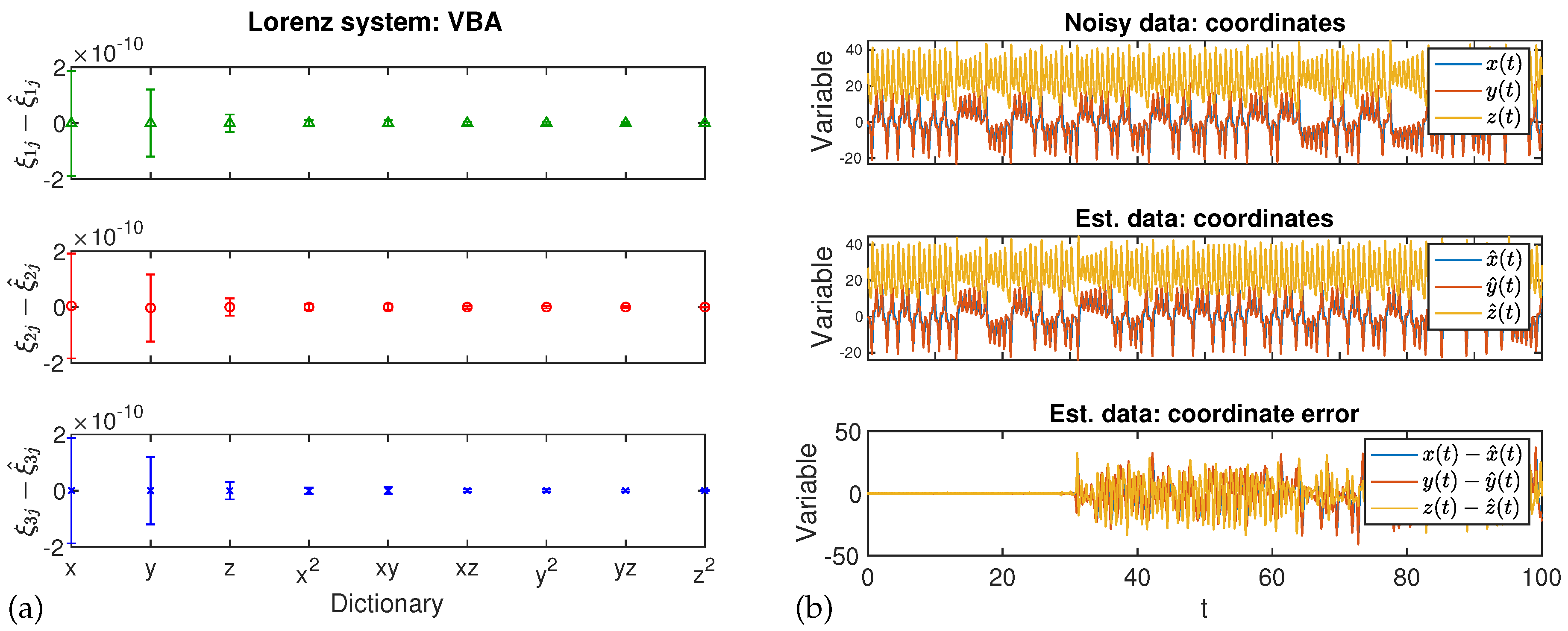
The calculated noisy data for the Lorenz system are illustrated in Figure 1a,b, respectively for the parameter values and their derivatives. The calculated regularization results are then presented in Figure 2, Figure 3 and Figure 4, respectively for the SINDy, JMAP and VBA methods. In each of these plots, the first subplot illustrates the difference in each inferred parameter (i.e., ), while the second subplot gives the inferred time series of the parameters , showing the noisy time series , the inferred series and their differences.
As evident in these plots, the three methods were approximately as effective in selection of the coefficients to recreate the Lorenz system. Of the other regularization methods published by [2], the iterative hard thresholding least squares and orthogonal matching pursuit also performed well, while the LASSO algorithm was unsuccessful for any system examined.
As noted, the two Bayesian methods also provided the variances of the predicted parameters, shown in Figure 3a and Figure 4a as error bars corresponding to the standard deviations. These calculations indicate the inferred parameter errors to be larger than previously appreciated, for example in the coefficient of x in all three series predicted by both JMAP and VBA. These values give a more realistic estimate of the inherent errors in the system identification method than suggested by the SINDy regularization.
5. Conclusions
We examine the problem of system identification of a dynamical system, represented by a nonlinear equation system , from discrete time series data. For this, we present a Bayesian inference framework based on the Bayesian maximum a posteriori (MAP) estimate, which for the assumption of Gaussian likelihood and prior functions, is shown to be equivalent to a variant of Tikhonov regularization. This Bayesian reinterpretation provides a clear theoretical justification for the choices of the residual and regularization terms, respectively as the negative logarithms of the likelihood and prior functions. The Bayesian approach is readily extended to the full apparatus of the Bayesian inverse solution, for example to quantify the uncertainty in the model parameters, or even to explore the functional form of the posterior pdf.
In this study, we compare the regularization method of least squares regression with thresholding (the SINDy algorithm) to two Bayesian methods JMAP and VBA, by application to the Lorenz system with added Gaussian noise. The Bayesian methods are shown to perform almost as effectively as SINDy for parameter estimation and reconstruction of the Lorenz time series. More importantly, the Bayesian methods also provide the variances – hence the standard deviations – of the inferred parameters, thereby giving a mathematical estimate of the system identification error. This is an important advantage of the Bayesian approach over traditional regularization methods.
Funding
This research was funded by the Australian Research Council Discovery Projects grant DP140104402, and also supported by French sources including Institute Pprime, CNRS, Poitiers, France, and CentraleSupélec, Gif-sur-Yvette, France.
Conflicts of Interest
The authors declare no conflict of interest. The funders had no role in the design of the study; in the collection, analyses, or interpretation of data; in the writing of the manuscript, or in the decision to publish the results.
References
- Brunton, S.L.; Proctor, J.L.; Kutz, J.N. Discovering governing equations from data by sparse identification of nonlinear dynamical systems. Proc. Natl. Acad. Sci. 2016, 113, 3932–3937. [Google Scholar] [CrossRef] [PubMed]
- Mangan, N.M.; Kutz, J.N.; Brunton, S.L.; Proctor, J.L. Model selection for dynamical systems via sparse regression and information criteria. Roy. Soc. Proc. A 2017, 473, 20170009. [Google Scholar] [CrossRef] [PubMed]
- Rudy, S.H.; Brunton, S.L.; Proctor, J.L.; Kutz, J.N. Data-driven discovery of partial differential equations. Sci. Adv. 2017, 3, e1602614. [Google Scholar] [CrossRef] [PubMed]
- Tikhonov, A.N. Solution of incorrectly formulated problems and the regularization method. Dokl. Akad. Nauk SSSR 1963, 151, 501–504. (In Russian) [Google Scholar]
- Santosa, F.; Symes, W.W. Linear inversion of band-limited reflection seismograms. SIAM J. Sci. Stat. Comp. 1986, 7, 1307–1330. [Google Scholar] [CrossRef]
- Tibshirani, R. Regression shrinkage and selection via the Lasso. J. R. Stat. Soc. B 1996, 58, 267–288. [Google Scholar] [CrossRef]
- Zhang, L.; Schaeffer, H. On the convergence of the SINDy algorithm. arXiv 2018, arXiv:1805.06445v1. [Google Scholar] [CrossRef]
- Brunton, S.L.; Brunton, B.W.; Proctor, J.L.; Kaiser, E.; Kutz, J.N. Koopman invariant subspaces and finite linear representations of nonlinear dynamical systems for control. PLoS ONE 2016, 11, e0150171. [Google Scholar] [CrossRef] [PubMed]
- Brunton, S.L.; Brunton, B.W.; Proctor, J.L.; Kaiser, E.; Kutz, J.N. Chaos as an intermittently forced linear system. Nat. Comm. 2017, 8, 19. [Google Scholar] [CrossRef] [PubMed]
- Taira, K.; Brunton, S.L.; Dawson, S.T.M.; Rowley, C.W.; Colonius, T.; McKeon, B.J.; Schmidt, O.T.; Gordeyev, S.; Theofilis, V.; Ukeiley, L.S. Modal analysis of fluid flows: An overview. AIAA J. 2017, 55, 4013–4041. [Google Scholar] [CrossRef]
- Mohammad-Djafari, A. Inverse problems in signal and image processing and Bayesian inference framework: From basic to advanced Bayesian computation. In Proceedings of the Scube Seminar, L2S, CentraleSupelec, At Gif-sur-Yvette, France., 27 March 2015. [Google Scholar]
- Mohammad-Djafari, A. Approximate Bayesian computation for big data. In Proceedings of the Tutorial at MaxEnt 2016, Ghent, Belgium, 10–15 July 2016. [Google Scholar]
- Teckentrup, A. Introduction to the Bayesian approach to inverse problems. In Proceedings of the MaxEnt 2018, Alan Turing Institute, UK, 6 July 2018. [Google Scholar]
- Lorenz, E.N. Deterministic nonperiodic flow. J. Atmos. Sci. 1963, 20, 130–141. [Google Scholar] [CrossRef]
Figure 1.
Calculated noisy data for the Lorenz system: (a) parameters , and (b) derivatives .

Figure 2.
Output of SINDy regularization: (a) differences in predicted parameters , and (b) comparison of original and predicted time series .
Figure 2.
Output of SINDy regularization: (a) differences in predicted parameters , and (b) comparison of original and predicted time series .
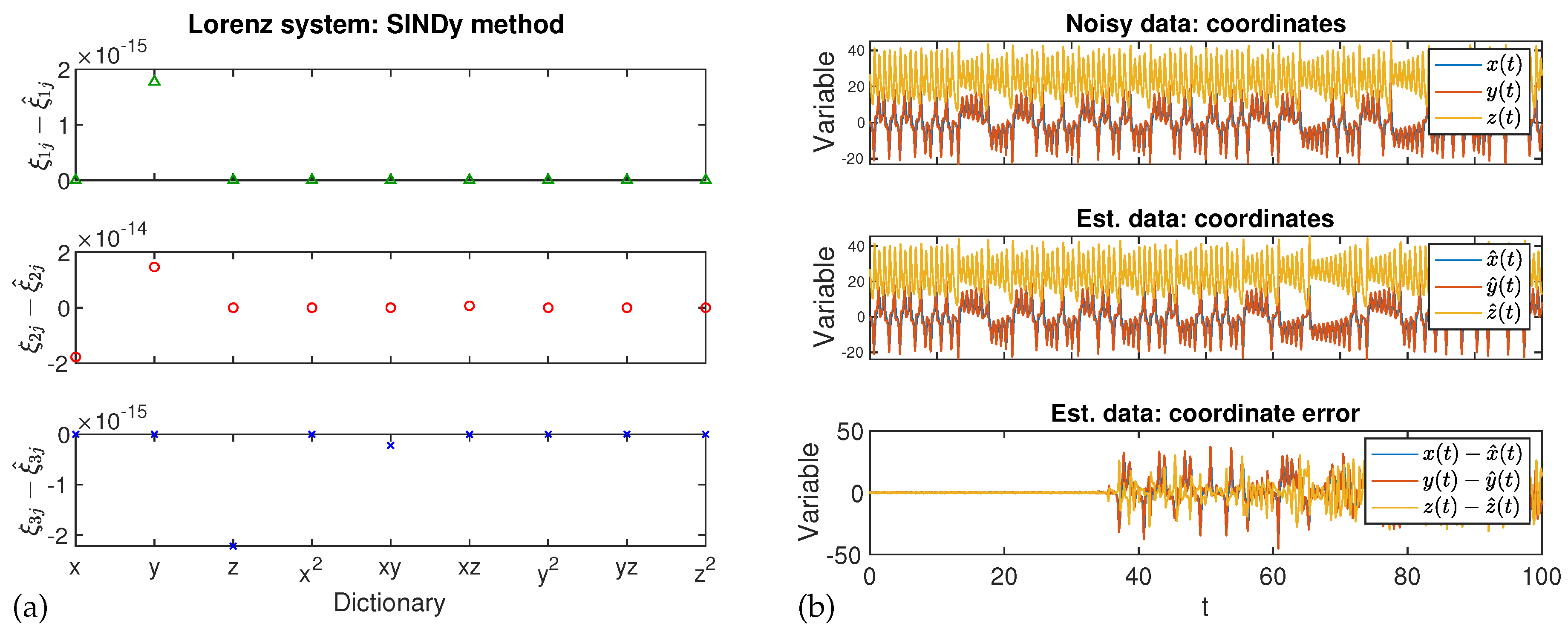
Figure 3.
Output of JMAP regularization: (a) differences in predicted parameters (the error bars indicate inferred standard deviations), and (b) comparison of original and predicted time series
Figure 3.
Output of JMAP regularization: (a) differences in predicted parameters (the error bars indicate inferred standard deviations), and (b) comparison of original and predicted time series
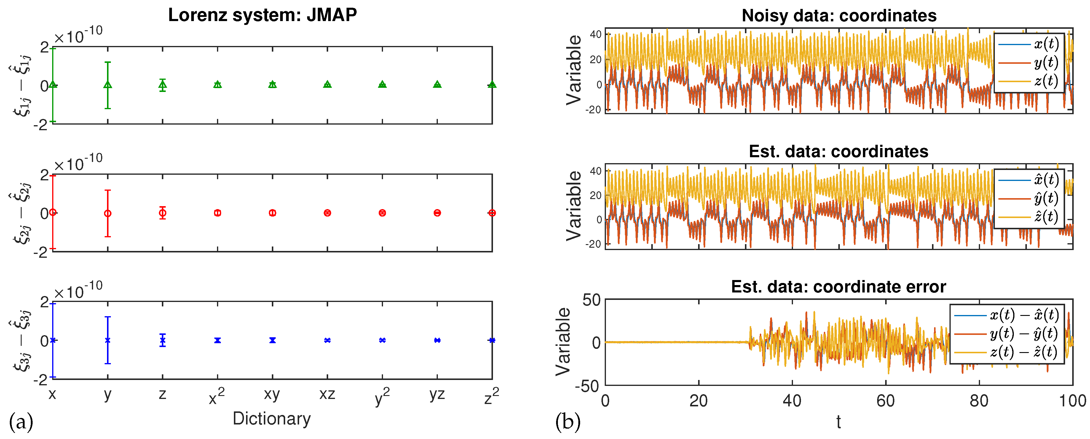
Figure 4.
Output of VBA regularization: (a) differences in predicted parameters (the error bars indicate inferred standard deviations), and (b) comparison of original and predicted time series .
Figure 4.
Output of VBA regularization: (a) differences in predicted parameters (the error bars indicate inferred standard deviations), and (b) comparison of original and predicted time series .
© 2020 by the authors. Licensee MDPI, Basel, Switzerland. This article is an open access article distributed under the terms and conditions of the Creative Commons Attribution (CC BY) license (http://creativecommons.org/licenses/by/4.0/).
Share and Cite
MDPI and ACS Style
Niven, R.K.; Mohammad-Djafari, A.; Cordier, L.; Abel, M.; Quade, M. Bayesian Identification of Dynamical Systems. Proceedings 2019, 33, 33. https://doi.org/10.3390/proceedings2019033033
AMA Style
Niven RK, Mohammad-Djafari A, Cordier L, Abel M, Quade M. Bayesian Identification of Dynamical Systems. Proceedings. 2019; 33(1):33. https://doi.org/10.3390/proceedings2019033033
Chicago/Turabian StyleNiven, Robert K., Ali Mohammad-Djafari, Laurent Cordier, Markus Abel, and Markus Quade. 2019. "Bayesian Identification of Dynamical Systems" Proceedings 33, no. 1: 33. https://doi.org/10.3390/proceedings2019033033