Estimating Flight Characteristics of Anomalous Unidentified Aerial Vehicles in the 2004 Nimitz Encounter ^†

Abstract

A number of Unidentified Aerial Phenomena (UAP) encountered by military, commercial, and civilian aircraft have been reported to be structured craft that exhibit ‘impossible’ flight characteristics. We consider the 2004 UAP encounters with the Nimitz Carrier Group off the coast of California, and estimate lower bounds on the accelerations exhibited by the craft during the observed maneuvers. Estimated accelerations range from $75\mathrm{g}$ to more than $5000\mathrm{g}$ with no observed air disturbance, no sonic booms, and no evidence of excessive heat commensurate with even the minimal estimated energies. In accordance with observations, the estimated parameters describing the behavior of these craft are both anomalous and surprising. The extreme estimated flight characteristics reveal that these observations are either fabricated or seriously in error, or that these craft exhibit technology far more advanced than any known craft on Earth. In the case of the Nimitz encounters the number and quality of witnesses, the variety of roles they played in the encounters, and the equipment used to track and record the craft favor the latter hypothesis that these are technologically advanced craft.

1. Introduction

Unidentified Aerial Phenomena (UAPs) partially identified as being unknown anomalous aircraft, referred to as Unidentified Anomalous Vehicles (UAVs) or Unidentified Flying Objects (UFOs), have been observed globally for some time [1]. Such phenomena were studied officially by the United States Air Force in a series of projects: Project Sign (1947), Project Grudge (1949) and Project Blue Book (1952–1969) [2]. Other nations, such as Australia, Brazil, Canada, Chile [3], Denmark, France, New Zealand, Russia (the former Soviet Union), Spain, Sweden, the United Kingdom, Uruguay, and the Vatican have also conducted studies, or are currently studying, UAPs [4]. In December of 2017 it was revealed that the United States government had been studying UAPs through at least one secret program called the Anomalous Aerospace Threat Identification Program (AATIP) [5], and that there have been times at which United States Naval pilots have had to deal with nearly daily encounters with UAVs [6,7]. These unidentified craft typically exhibit anomalous flight characteristics, such as traveling at extremely high speeds, changing direction or accelerating at extremely high rates, and hovering motionless for long periods of time. Furthermore, these craft appear to violate the laws of physics in that they do not have flight or control surfaces, any visible means of propulsion apparently violating Newton’s Third Law, and can operate in multiple media, such as space (low Earth orbit), air, and water without apparent hindrance, sonic booms, or heat dumps [4].

The nature, origin, and purpose of these UAVs are unknown. It is also not known if they are piloted, controlled remotely, or autonomous. If some of these UAVs are of extraterrestrial origin, then it would be important to assess the potential threat they pose [4]. More interestingly, these UAVs have the potential to provide new insights into aerospace engineering and other technologies [8]. The potential of a serious threat as well as the promise of advancements in science and engineering, along with our evolving expectations about extraterrestrial life are important reasons for scientists to seriously study and understand these objects [9,10,11,12,13]. We carefully examine a series of encounters in 2004 by pilots and radar operators of the Nimitz carrier group, and estimate lower bounds on their accelerations. We demonstrate that the estimated accelerations are indeed extraordinary and surprising.

2. Nimitz Encounters (2004)

For a two week period in November of 2004, the U.S. Navy’s Carrier Strike Group Eleven (CSG-11), which includes the USS Nimitz nuclear aircraft carrier and the Ticonderoga-class guided missile cruiser USS Princeton, encountered as many as 100 UAVs. We estimated the accelerations of UAVs relying on (1) radar information from USS Princeton former Senior Chief Operations Specialist Kevin Day; (2) eyewitness information from CDR David Fravor, commanding officer of Strike Fighter Squadron 41 and the other jet’s weapons system operator, LCDR Jim Slaight; and (3) analyses of a segment of the Defense Intelligence Agency-released Advanced Targeting Forward Looking Infrared (ATFLIR) video. The following descriptions of the Nimitz encounters were summarized from the more detailed study published by the Scientific Coalition for UAP Studies (SCU) [14].

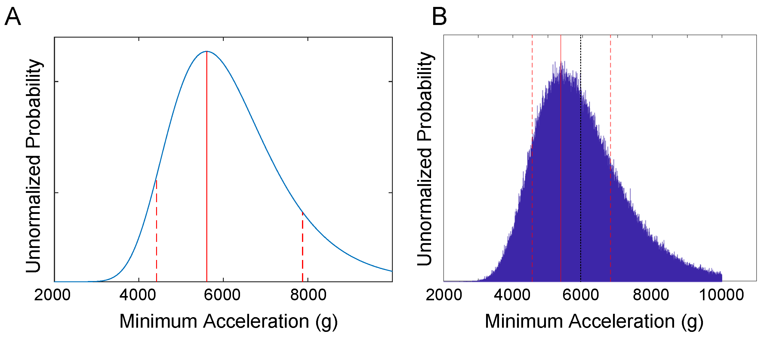
2.1. Senior Chief Operations Specialist Kevin Day (RADAR)

An important role of the USS Princeton is to act as air defense protection for the strike group. The Princeton was equipped with the SPY-1 radar system which provided situational awareness of the surrounding airspace. The main incident occurred on 14 November 2004, but several days earlier, radar operators on the USS Princeton were detecting UAVs appearing on radar at about 80,000+ feet altitude to the north of CSG-11 in the vicinity of Santa Catalina and San Clemente Islands. Senior Chief Kevin Day informed us that the Ballistic Missile Defense (BMD) radar systems had detected the UAVs in low Earth orbit before they dropped down to 80,000 feet [15]. The UAVs would arrive in groups of 10 to 20, subsequently drop down to 28,000 feet with a several hundred foot variation, and track south at a speed of about 100 knots [15]. Periodically, the UAVs would drop from 28,000 feet to sea level (approx. 50 feet), or under the surface, in 0.78 seconds. Without detailed radar data, it is not possible to know the acceleration of the UAVs as a function of time as they descended to the sea surface. However, one can estimate a lower bound on the acceleration by assuming that the UAVs accelerated at a constant rate halfway and then decelerated at the same rate for the remaining distance so that

$$\frac{1}{2}d=\frac{1}{2}a{\left(\frac{t}{2}\right)}^2.$$

(1)

The data consisted of the change in altitude $y\pm {\sigma }_y=8530\pm 90\mathrm{m}$ ($-28,000\mathrm{ft}\pm 295\mathrm{ft}$) and the duration $t^{\prime }\pm {\sigma }_t=0.78\pm 0.08\mathrm{s}$, where the goal was to estimate the acceleration, a. The dominant source of uncertainty in altitude was due to the observed variation in altitude among the observed UAVs, which was on the order of 200 to $300\mathrm{ft}$.

In the first analysis, we assigned a joint Gaussian likelihood, $P(y,t|a,I)$ for the measured altitude change and the duration of the maneuver. Since the altitude change and the duration are independently measured, the joint likelihood is factored into the product of two likelihoods, and one can marginalize over the duration of the maneuver to obtain a likelihood for the altitude y

$$\begin{array}{cc}\hfill P\left(y\right|a,I)& ={\int }_{-\infty }^{\infty }dtP(y,t|a,{\sigma }_y,t^{\prime },{\sigma }_t,I)\hfill \end{array}$$

(2)

$$\begin{array}{cc}\hfill & ={\int }_{-\infty }^{\infty }dtP\left(y\right|a,t,{\sigma }_y,I)P\left(t\right|t^{\prime },{\sigma }_t,I),\hfill \end{array}$$

(3)

where the symbol I represents the fact that these probabilities are conditional on all prior information. Assigning Gaussian likelihoods we have that

$$\begin{array}{cc}\hfill P\left(y\right|a,I)& ={\int }_{-\infty }^{\infty }dt\frac{1}{\sqrt{2\pi }{\sigma }_y}exp\left[-\frac{1}{2{\sigma }_y^2}{\left(y+\frac{1}{4}a{t}^2\right)}^2\right]\frac{1}{\sqrt{2\pi }{\sigma }_t}exp\left[-\frac{1}{2{\sigma }_t^2}{\left(t-t^{\prime }\right)}^2\right]\hfill \end{array}$$

(4)

$$\begin{array}{cc}\hfill & =\frac{1}{2\pi {\sigma }_y{\sigma }_t}{\int }_{-\infty }^{\infty }dtexp\left[-\frac{1}{2{\sigma }_y^2}{\left(y+\frac{1}{4}a{t}^2\right)}^2-\frac{1}{2{\sigma }_t^2}{\left(t-t^{\prime }\right)}^2\right].\hfill \end{array}$$

(5)

The integrand is the exponential of a quartic polynomial in t, which was solved numerically. Assigning a uniform prior probability for the acceleration over a wide range of possible accelerations results in a posterior that is proportional to the likelihood (4) above resulting in a maximum likelihood analysis, which gave an estimate of $a=5600\begin{array}{c}+2270\\ -1190\end{array}$$\mathrm{g}$, as illustrated in Figure 1A.

As a second analysis, we employed sampling for which the change in altitude and the elapsed time were described by Gaussian distributions with $y\pm {\sigma }_y=8530\pm 90\mathrm{m}$ and $t^{\prime }\pm {\sigma }_t=0.78\pm 0.08\mathrm{s}$, respectively. The most probable acceleration was 5370$\begin{array}{c}+1430\\ -820\end{array}$$\mathrm{g}$ while the mean acceleration was $5950\mathrm{g}$ (Figure 1B).

With acceleration estimates in hand, we obtained a ballpark estimate of the power involved to accelerate the UAV. Of course, this required an estimate of the mass of the UAV, which we did not have. The UAV was estimated to be approximately the same size as an F/A-18 Super Hornet, which has a weight of about $32,000\mathrm{lbs}$, corresponding to $14,550\mathrm{kg}$. Since we want a minimal power estimate, we took the acceleration as $5370\mathrm{g}$ and assumed that the UAV had a mass of $1000\mathrm{kg}$. The UAV would have then reached a maximum speed of about $46,000\mathrm{mph}$ during the descent, or 60 times the speed of sound, at which point the required power peaked at a shocking $1100\mathrm{GW}$, which exceeds the total nuclear power production of the United States by more than a factor of ten. For comparison, the largest nuclear power plant in the United States, the Palo Verde Nuclear Generating Station in Arizona, provides about $3.3\mathrm{GW}$ of power for about four million people [16].

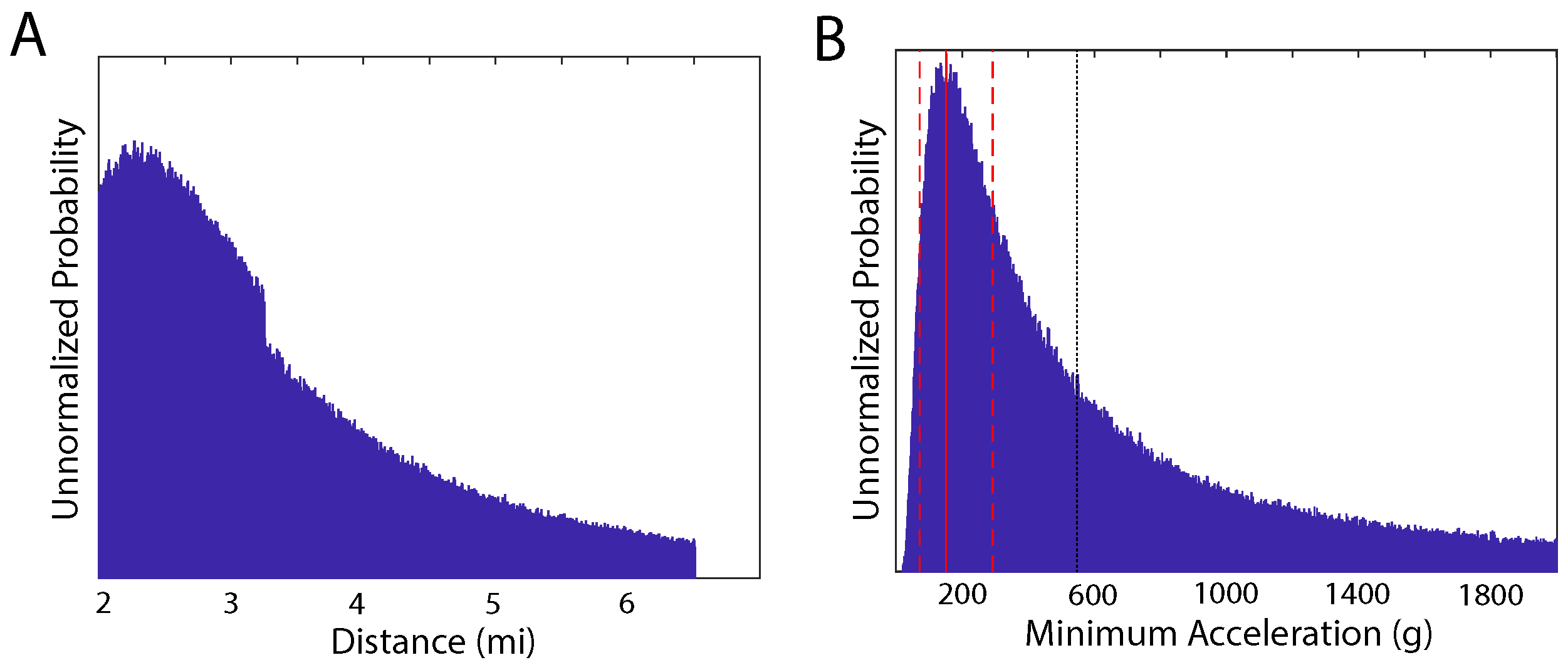
2.2. Commander David Fravor (PILOT)

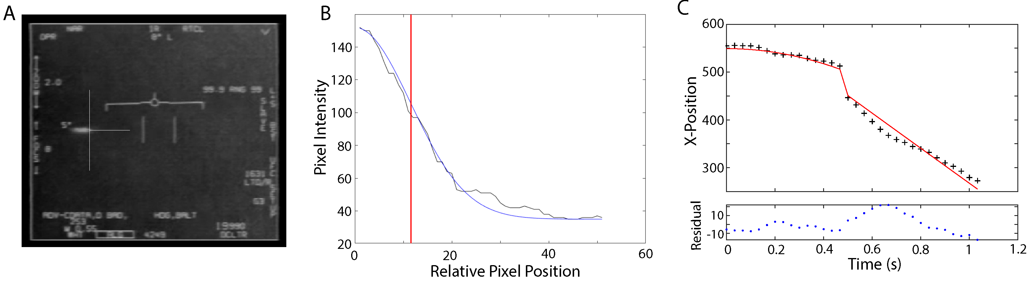
On Nov. 14, 2004, CSG-11 was preparing for training exercises. Two F/A-18F Super Hornets were launched from the Nimitz for the air defense exercise to be conducted in an area 80–150 miles SSW of San Diego. Both planes, with call signs “FastEagle01” and “FastEagle02”, had a pilot and a weapons system operator (WSO) onboard. VFA-41 Squadron Commanding Officer David Fravor was piloting FastEagle01 and LCDR Jim Slaight was the WSO of FastEagle02. CDR Fravor and his wingman were headed for the Combat Air Patrol (CAP) point, which is given by predefined latitude, longitude and altitude coordinates, where they would conduct the training exercises.

About a half-hour after take-off, Senior Chief Day operating the SPY-1 radar system on the Princeton detected UAVs entering the training area. The training exercise was delayed and FastEagle01 and FastEagle02 were directed to intercept a UAV at a distance of 60 miles and an altitude of 20,000 feet. As the F-18s approached merge plot, which is the point at which the radar could not differentiate the positions of the F-18s and the UAV, Fravor and Slaight noticed a disturbed patch of water, where it appeared as if there was a large object, possibly a downed aircraft, submerged 10 to 15 feet below the surface. As they observed the disturbance from 20,000 ft, all four pilots spotted a white UAV, shaped like a large cylindrical butane tank, or a Tic-Tac candy, moving erratically back and forth, almost like a bouncing ping-pong ball making instantaneous changes in direction without changing speed. The Tic-Tac UAV was estimated to be about the size of an F-18, about 40–50 feet in length and 10–15 feet wide, but had no apparent flight surfaces or means of propulsion, and its movement had no apparent effect on the ocean surface as one would expect from something like rotor wash from a helicopter.

Fravor started a descent to investigate while his wingman kept high cover. As Fravor circled and descended, the UAV appeared to take notice of him and rose to meet him. The F-18 and the UAV circled one another. When Fravor reached the nine o’clock position, he performed a maneuver to close the distance by cutting across the circle to the three o’clock position. As he did so, the Tic-Tac UAV accelerated ([14], p.12) across Fravor’s nose heading south. Fravor said that the UAV was gone within a second. As a comparison, Fravor noted that even a jet at Mach 3 takes 10 to 15 seconds to disappear from sight ([14], p.11). LCDR Slaight described the UAV as accelerating as if it was “shot out of a rifle” and that it was out of sight in a split second. ([14], p. 12).

The engagement lasted five minutes. With the Tic-Tac gone, the pilots turned their attention toward the large object in the water, but the disturbance has disappeared. The two FastEagles returned to the Nimitz, without sufficient fuel to attempt to pursue the Tic-Tac. On their way back, they received a call from the Princeton that the Tic-Tac UAV was waiting precisely at their CAP point. Senior Chief Day noted that this was surprising because those coordinates were predetermined and secret. Given that the CAP point was approximately $R=60\mathrm{mi}$ away, the probability of selecting the CAP point out of all the locations within the 60 mile radius, to within a one mile resolution (slightly more than the resolution of the radar system), is

$$P\left(x\right|I)=\frac{1}{\pi R^2}=\frac{1}{11310}=0.0088\%,$$

(6)

discounting the altitude. It appears that the Tic-Tac UAV intentionally went to that location, although it is not clear how this would be possible.

To obtain a lower bound on the acceleration, we assume that the UAV exhibited constant acceleration so that the distance traveled was given by

$$d=\frac{1}{2}a{t}^2$$

(7)

during the elapsed time. The length of the Tic-Tac UAV was estimated to be about $40\mathrm{ft}$ with a cross sectional width of about $w=10\mathrm{ft}$. Given that the acuity of human vision is about $\theta =1/{60}^{\circ }$ the UAV, at its narrowest, would be out of sight at a maximum distance of

$$d=\frac{w/2}{tan(\theta /2)},$$

(8)

which is $d\approx 6.5\mathrm{mi}$. It is difficult to know what Fravor’s acuity was given the viewing conditions. For this reason, we model the acuity conservatively as a truncated Gaussian distribution with a peak at $\theta =1/{30}^{\circ }\pm 1/{60}^{\circ }$. The truncation at $\theta =1/{60}^{\circ }$ resulted in a discontinuity in the distribution of the distances (Figure 2A), which peaks around $2.25\mathrm{mi}$.

The elapsed time is modeled as a Gaussian distribution with a mean of $1\pm 1\mathrm{s}$ and truncated for positive values of time. The resulting acceleration distribution was a skewed distribution of accelerations (Figure 2B) with a most probable acceleration of $150\begin{array}{c}+140\\ -80\end{array}\mathrm{g}$, indicated in the figure by the red vertical lines and a mean acceleration of about $550\mathrm{g}$ indicated by the black vertical dotted line. Note that this is a lower bound, probably far below the observed acceleration if the UAV accelerated briefly as if “shot out of a rifle” and then traveled at a constant speed.

2.3. ATFLIR Video

Upon returning to the Nimitz, CDR Fravor requested that a crew equipped with the ATFLIR pod obtain videos of the Tic-Tac UAV. Two F/A-18Fs were launched under the guidance of an E-2 Hawkeye airborne radar plane. The two planes separated in search of the UAV, with one plane heading south toward the CAP point where the UAV was last seen on radar. That plane picked up a contact 33 miles to the south on the Range While Search (RWS) scan. This Tic-Tac UAV was filmed using the ATFLIR system, and the video was released to the public as the “Nimitz video” (Figure 3A).

We examined the last 32 frames of the Nimitz video in which the Tic-Tac UAV accelerated to the left and the targeting system lost lock. The video frame rate was $29.97\mathrm{frames}/\mathrm{s}$. As the UAV accelerates the image of the UAV becomes elongated and blurred. If the shutter speed was known, then this information could be used to better estimate the speed of the craft. This could be accomplished by treating the shutter speed as a model parameter, but such analysis is beyond the scope of this project. Instead, we concentrated on tracking the position of the right edge of the UAV and using those positions to estimate the kinematics. The left edge of the UAV was also estimated in the first frame to provide some information about the range, $z_o$, to the UAV given that that UAV was estimated to be about 40 feet in length. However, since the orientation was not known, this is modeled as a uniformly distributed unknown angular parameter $\varphi \in \{0,3\pi /8\}$, which allowed one to at least put an upper bound on the range $z_o$.

To estimate the position of the right edge of the craft in each frame (Figure 3A), the row of pixels for which the UAV has a maximum intensity was examined. The pixel intensities along that row at the right edge of the UAP were fit (maximum likelihood method with a Student-t likelihood) to half of a Gaussian curve. The center position of the Gaussian plus the standard deviation was used as the position of the right side of the UAV for that frame (Figure 3B).

Horizontal positions of the UAV are related to the pixel coordinates by noting that the entire field of view (approximately $FO{V}_{pix}=606\mathrm{pixels}$) corresponds to an angular field of view of $0.7^{\circ }$ in the narrow (NAR) mode, which is indicated in the upper left hand corner of the video. At the range, $z_o$, of the UAV this results in the proportion

$$X_{scale}=\frac{FO{V}_{pix}/2}{z_{o}tan\frac{0.7^{\circ }}{2}}$$

(9)

where $X_{scale}$ has units $\frac{\mathrm{pixels}}{\mathrm{m}}$ when $z_o$ is in units of $\mathrm{m}$. The ATFLIR has a zoom feature that can change the field of view. In the Nimitz video frames analyzed, the zoom is first set to unity in the NAR mode so that the angular field of view is $0.7^{\circ }$. However, at frame 16, the zoom changes to two, so that the angular field of view in the NAR mode changes to $0.{35}^{\circ }$. This appears as a discontinuity in the data (‘+’ symbols) illustrated in Figure 3C.

We analyzed four different kinematic models using nested sampling, and statistically tested them by comparing the log Bayesian evidence. We used uniform prior probabilities for the kinematic parameters as well as a Student-t likelihood function, which is robust to outliers, such as those due to camera (airplane) motion. Model #1 considers constant acceleration to the left (-x direction). Model #2 considers constant acceleration both to the left (-x direction) and toward or away from the camera (z-direction). The forward model provides the position of the UAV as a function of time, where $t_i$ is the time of the $i^{th}$ video frame:

$$\mathrm{Models} \#1 \mathrm{and} \#2 \begin{array}{c}\left\{\begin{array}{cc}x\left(t_i\right)\hfill & =\frac{1}{2}{a}_x{t_i}^2+x_o\hfill \\ z\left(t_i\right)\hfill & =\frac{1}{2}{a}_z{t_i}^2+z_o\hfill \end{array}\right.\mathrm{const}.\mathrm{accel}.,\end{array}$$

(10)

for which $a_x\in [-200,0]\mathrm{g}$, $a_z\in [-100,100]\mathrm{g}$, $x_o\in [-100,100]\mathrm{px}$, $z_o\in [7.57,75.75]\mathrm{mi}$, and Model #1 just considers the UAV’s acceleration in the x-direction (to the left) so that $a_z\doteq 0$.

Models #3 and #4 describe the kinematics as constant acceleration followed by constant velocity motion after Frame 15:

$$\mathrm{Models} \#3 \mathrm{and} \#4\begin{array}{c}\left\{\begin{array}{cc}x\left(t_i\right)\hfill & =\frac{1}{2}{a}_x{t_i}^2+x_o\mathrm{for}{t}_i<t_{16}\hfill \\ x\left(t_i\right)\hfill & =\frac{1}{2}{a}_x{t_{15}}^2+a_x{t}_{15}(t_i-t_{15})+x_o\mathrm{for}{t}_i\ge t_{16}\hfill \\ z\left(t_i\right)\hfill & =\frac{1}{2}{a}_z{t_i}^2+z_o\mathrm{for}{t}_i<t_{16}\hfill \\ z\left(t_i\right)\hfill & =\frac{1}{2}{a}_z{t_{15}}^2+a_z{t}_{15}(t_i-t_{15})+z_o\mathrm{for}{t}_i\ge t_{16}\hfill \end{array}\right.\end{array}$$

(11)

for which $a_x\in [-200,0]\mathrm{g}$, $a_z\in [-100,100]\mathrm{g}$, $x_o\in [-100,100]\mathrm{px}$, $z_o\in [7.57,75.75]\mathrm{mi}$, and Model #3 just considers the UAV’s acceleration in the x-direction (to the left) so that $a_z\doteq 0$.

The models were analyzed using a nested sampling algorithm [17,18], which allowed for the estimation of the logarithm of the Bayesian evidence, logZ, as well as the logarithm of the likelihood, logL, and mean estimates of the model parameters. The analysis was performed for $N=500$ samples and was run until the change in logZ from successive iterations was less than ${10}^{-5}$, ensuring a reliable estimate of the log evidence. Tests were performed to ensure that the trial-to-trial variations in parameter estimates were within the estimated uncertainties.

The results of the nested sampling analysis are listed in

Table 1. Kinematic Models for the Nimitz Video Given the log evidence (logZ), Model 4 (bold) is most probable with a net acceleration of $75.9\pm 0.2\mathrm{g}$.

Model	logZ	LogL	${\mathit{a}}_{\mathit{x}}\left(\mathbf{g}\right)$	${\mathit{a}}_{\mathit{z}}\left(\mathbf{g}\right)$	${\mathit{x}}_{\mathit{o}}\left(\mathbf{m}\right)$	${\mathit{z}}_{\mathit{o}}\left(\mathbf{m}\right)$
Model 1	$-253,640$	$-253,614$	$-71.1\pm 0.7$	–	$-15.40\pm 0.04$	$119,700\pm 1200$
Model 2	$-236,950$	$-236,287$	$7.564\pm 0.002$	$99.994\pm 0.005$	$-13.36\pm 0.04$	$12,193\pm 1$
Model 3	$-53,282$	$-53,261$	$-40.2\pm 3.8$	–	$-4.02\pm 0.05$	$49,700\pm 4800$
Model 4	$-\mathbf{52},\mathbf{084}$	$-\mathbf{52},\mathbf{031}$	$-\mathbf{35}.\mathbf{64}\pm \mathbf{0}.\mathbf{08}$	$\mathbf{67}.\mathbf{04}\pm \mathbf{0}.\mathbf{18}$	$-\mathbf{3}.\mathbf{89}\pm \mathbf{0}.\mathbf{05}$	$\mathbf{43},\mathbf{870}\pm \mathbf{110}$

. The uncertainties in the logZ estimates (not listed) were on the order of one or less. Model 4, which describes the motion of the UAV as a constant acceleration to the left and away from the observer for the first 15 frames (approximately $0.53\mathrm{s}$), is the most probable solution with acceleration components of $a_x=-35.64\pm 0.08\mathrm{g}$ and $a_z=67.04\pm 0.18\mathrm{g}$ for a net acceleration of about $75.9\pm 0.2\mathrm{g}$. The residuals indicate that a more precise model would consist of multiple episodes of acceleration during the maneuver. This was observed in SCU’s analysis [14] where the accelerations were estimated to vary from around 40 to $80\mathrm{g}$.

A more detailed analysis would involve modeling the motion of the UAV more precisely by modeling the pixel intensities on the video frames themselves. By considering the shutter speed, the blurring of the UAV image due to its motion would provide more information about its speed. In addition, the “change points” at which the accelerations changed could be treated as model parameters allowing for a more precise description of the UAV’s behavior.

3. Discussion

In this paper, we have worked under the assumption that these UAPs were physical craft as described by the pilots. The fact that these UAPs exhibited astonishing flight characteristics leaves one searching for other possible explanations. One very clever explanation suggested by one of the reviewers was that these UAPs could have been generated by the intersection of two or more laser or maser beams ionizing the air, which could create a visual image, an infrared image, as well as a radar reflective region possibly explaining much of the observations.

While such an explanation could explain the visual, infrared and radar observations, it would not be able to explain either the suborbital radar returns from the ballistic missile defense (BMD) radar systems on the Princeton before the UAPs dropped to $80,000\mathrm{ft}$, or the sonar returns when the TicTac UAPs went into the ocean [15], both of which are not as well substantiated or documented as the other observations.

More importantly, the distribution of the UAPs ranged from over 100 miles to the north over Catalina Island to about 70 miles to the west. This would require an array of widely distributed and coordinated lasers situated on multiple ships or aircraft. However, it is known that there were no other ships or airplanes in the area. In addition, the fact that the UAP reacted to CDR Fravor’s maneuvers would require that radar be used to track the F-18s so that the laser-produced imagery could react to them. However, any such radar frequencies being used in the area would have been detected by the Princeton, the E-2 Hawkeye, and the F-18s themselves.

If any such system were being secretly tested against CSG-11, one would expect it to mimic real-life events, such as an enemy aircraft, drone, or missile launch. But the UAPs and their behavior were nothing like this. Furthermore, such powerful lasers might endanger the planes or personnel if anything went wrong in the testing, and the fact that the pilots were forced to take evasive maneuvers [19] reveals that they were being put in harms way. One wouldn’t need to test a system in this manner, and if such a test did take place it would very likely have been illegal. Furthermore, such an explanation would have difficulty explaining the almost daily encounters experienced by pilots in the Roosevelt Carrier Group both off the coast of Virginia and during military operations in the Persian Gulf [6,7], or earlier encounters, such as that by Lt. Bethune in 1951, two years before the invention of the maser and nine years before the invention of the laser, which was analyzed in the extended version of this paper [20].

4. Conclusions

We have carefully considered a set of encounters between the Nimitz CSG-11 and UAPs of unknown nature and origin. Much of the information available consisted of eyewitness descriptions made by multiple trained witnesses observing in multiple modalities including visual contact from pilots, radar, and infrared video. While fabrication and exaggeration cannot be ruled out, the fact that multiple professional trained observers working in different modalities corroborate the reports greatly minimizes such risks.

The analysis aimed to estimate lower bounds on the acceleration. This was found by assuming that the UAVs accelerated a constant rate. We worked to obtain conservative estimates by assigning liberal uncertainties. It was found that the minimum acceleration estimates, ranging from about $70\mathrm{g}$ to well over $5000\mathrm{g}$, far exceeded those expected for an aircraft (

Table 2. Summary of Estimated Accelerations ranging from about $75\mathrm{g}$ to over $5300\mathrm{g}$. Detection Modalities refer to Multiple Pilots Visual Contact (Vs), Radar (R), Infrared Video (IR).

Case	Detection Modalities	Kinematic Model	Figure	Min. Acceleration
Day	R	(1)	Figure 1B	5370$\begin{array}{c}+1430\\ -820\end{array}$$\mathrm{g}$
Fravor	R,Vs	(7)	Figure 2C	150$\begin{array}{c}+140\\ -80\end{array}$$\mathrm{g}$
ATFLIR	R,Vs,IR	(11)	Figure 3C	$75.9\pm 0.2\mathrm{g}$

). For comparison, humans can endure up to $45\mathrm{g}$ for $0.044\mathrm{s}$ with no injurious or debilitating effects, but this limit decreases with increasing duration of exposure [21]. For durations more than $0.2\mathrm{s}$ the limit of tolerance decreases to $25\mathrm{g}$ and it decreases further still for longer durations [21].

These considerations suggest that these UAVs may not have been piloted, but instead may have been remote controlled or autonomous. However, it should be noted that even equipment can only handle so much acceleration. For example, the Lockheed Martin F-35 Lightning II has maintained structural integrity up to $13.5\mathrm{g}$ [22]. Missiles can handle much higher accelerations. The Crotale NG VT1 missile has an airframe capable of withstanding $50\mathrm{g}$ and can maintain maneuverability up to $35\mathrm{g}$ [23]. However, these accelerations are still only about half of lowest accelerations that we have estimated for these UAVs. The fact that these UAVs display no flight surfaces or apparent propulsion mechanisms, and do not produce sonic booms or excessive heat that would be released given the hundreds of GigaWatts of power that we expect should be involved, strongly suggests that these anomalous craft are taking advantage of technology, engineering, or physics that we are unfamiliar with. For example, the Tic-Tac UAV dropping from $28,000\mathrm{ft}$ to sea level in $0.78\mathrm{s}$ involved at least $4.3\times {10}^{11}\mathrm{J}$ of energy (assuming a mass of $1000\mathrm{kg}$), which is equivalent to about 100 tons of TNT, or the yield of 200 Tomahawk cruise missiles, released in $\frac{3}{4}$ of a second. One would have expected a catastrophic effect on the surrounding environment. This does not rule out the possibility that these UAVs have been developed by governments, organizations, or individuals on Earth, but it suggests that these UAVs and the technologies they employ may be of extraterrestrial origin. That being said, it should be strongly emphasized that proving that something is extraterrestrial would be extremely difficult, even if one had a craft in hand.

The purpose of this paper is to focus on the flight kinematics of these UAVs with the aim of building up a body of scientific evidence that will allow for a more precise understanding of their nature and origin.

As such, it is difficult to draw any useful conclusions at this point. We have characterized the accelerations of a number of UAVs and have demonstrated that if they are craft then they are indeed anomalous, displaying technical capabilities far exceeding those of our fastest aircraft and spacecraft. It is not clear that these objects are extraterrestrial in origin, but it is extremely difficult to imagine that anyone on Earth with such technology would not put it to use. Moreover, observations of similar UAPs go back to well before the era of flight [1]. Collectively, these observations strongly suggest that these UAVs should be carefully studied by scientists [9,10,11,12,13].

Unfortunately, the attitude that the study of UAVs (UFOs) is “unscientific” pervades the scientific community, including SETI (Search for Extraterrestrial Intelligence) [24], which is surprising, especially since efforts are underway to search for extraterrestrial artifacts in the solar system [25,26,27,28,29], in particular, on the Moon, Mars, asteroids [30], and at Earth-associated Lagrange points. Ironically, such attitudes inhibit scientific study, perpetuating a state of ignorance about these phenomena that has persisted for well over 70 years, and is now especially detrimental, since answers are presently needed [31,32,33,34].

References

1. Vallee, J.; Aubeck, C. Wonders in the Sky: Unexplained Aerial Objects from Antiquity to Modern Times; Penguin: New York, NY, USA, 2010. [Google Scholar]
2. Unidentified Flying Objects and Air Force Project Blue Book. Available online: https://web.archive.org/web/20030624053806/http://www.af.mil/factsheets/factsheet.asp?fsID=188 (accessed on 9 June 2019).
3. CEFAA. Comité de Estudios de Fenómenos Aéreos Anómalos. Available online: http://www.cefaa.gob.cl/ (accessed on 27 July 2019).
4. Elizondo, L. The imminent change of an old paradigm: The U.S. government’s involvement in UAPs, AATIP, and TTSA. In Proceedings of the Anomalous Aerospace Phenomena Conference (AAPC 2019) Presentation, Huntsville, AL, USA, 15–17 March 2019. [Google Scholar]
5. Cooper, H.; Blumenthal, R.; Kean, L. Glowing auras and “black money”: The Pentagon’s mysterious U.F.O. program. The New York Times.
6. Stieb, M. Navy pilots were seeing UFOs on an almost daily basis in 2014 and 2015: Report. New York Magazine, 2019. Available online: http://nymag.com/intelligencer/2019/05/navy-pilots-are-seeing-ufos-on-an-almost-daily-basis-report.html(accessed on 24 July 2019).
7. Rogoway, T. Recent UFO Encounters with Navy pilots occurred constantly across multiple squadrons. The Drive, 2019. Available online: https://www.thedrive.com/the-war-zone/28627/recent-ufo-encounters-with-navy-pilots-occurred-constantly-across-multiple-squadrons(accessed on 24 July 2019).
8. Monzon, I. Tech CEOs want to capture UFOs and reverse engineer them. International Business Times, 2019. Available online: https://www.ibtimes.com/tech-ceos-want-capture-ufos-reverse-engineer-them-2803920,(accessed on 24 July 2019).
9. Hynek, J.A. The UFO Experience: A Scientific Inquiry; Henry Regnery: Chicago, IL, USA, 1972. [Google Scholar]
10. Hill, P.R. Unconventional Flying Objects: A Scientific Analysis; Hampton Roads Publishing Co.: Charlottesville, VA, USA, 1995. [Google Scholar]
11. Sturrock, P.A. The UFO Enigma: A New Review of the Physical Evidence; Aspect: New York, NY, USA, 2000. [Google Scholar]
12. Knuth, K.H. Are we alone? The question is worthy of serious scientific study. The Conversation. 2018. Available online: https://theconversation.com/are-we-alone-the-question-is-worthy-of-serious-scientific-study-98843 (accessed on 24 July 2018).
13. Colombano, S.P. New Assumptions to Guide SETI Research. 2018. Available online: https://ntrs.nasa.gov/archive/nasa/casi.ntrs.nasa.gov/20180001925.pdf (accessed on 24 July 2018).
14. Powell, R.; Reali, P.; Thompson, T.; Beall, M.; Kimzey, D.; Cates, L.; Hoffman, R. A Forensic Analysis of Navy Carrier Strike Group Eleven’s Encounter with an Anomalous aerial Vehicle. 2019. Available online: https://www.explorescu.org/post/nimitz_strike_group_2004 (accessed on 9 July 2018).
15. Day, K. (U.S. Navy (ret.)). Private Communication, 2019. [Google Scholar]
16. Palo Verde Nuclear Generating Station. Available online: https://en.wikipedia.org/wiki/Palo_Verde_Nuclear_Generating_Station (accessed on 8 Augest 2018).
17. Skilling, J. Nested sampling for general Bayesian computation. Bayesian Anal. 2006, 1, 833–859. [Google Scholar] [CrossRef]
18. Sivia, D.S.; Skilling, J. Data Analysis. A Bayesian Tutorial, second ed.; Oxford University Press: Oxford, 2006. [Google Scholar]
19. 2004 Nimitz Pilot Report. 2017. Available online: https://thevault.tothestarsacademy.com/nimitz-report (accessed on 7 October 2018).
20. Knuth, K.H.; Powell, R.M.; Reali, P.A. Estimating Flight Characteristics of Anomalous Unidentified Aerial Vehicles. Entropy 2019, 21, 939. [Google Scholar] [CrossRef]
21. Eiband, A.M. Human Tolerance to Rapidly Applied Accelerations: A Summary of the Literature. 1959. Available online: https://ntrs.nasa.gov/archive/nasa/casi.ntrs.nasa.gov/19980228043.pdf (accessed on 27 July 2019).
22. Kent, J. F-35 Lightning II News. 2010. Available online: http://www.f-16.net/f-35-news-article4113.html (accessed on 27 July 2019).
23. Army-Technology.com. Crotale NG Short Range Air Defence System. Available online: https://www.army-technology.com/projects/crotale/ (accessed on 27 July 2019).
24. Wright, J. Searches for technosignatures: The state of the profession. arXiv 2019, arXiv:1907.07832. [Google Scholar]
25. Bracewell, R. Communications from superior galactic communities. Nature 1960, 186, 670–671. [Google Scholar] [CrossRef]
26. Bracewell, R. Interstellar probes. In Interstellar Communication: Scientific Perspectives; Ponnamperuma, C., Cameron, A.G.W., Eds.; Houghton-Mifflin: Boston, MA, USA, 1974; pp. 141–167. [Google Scholar]
27. Freitas, R.A., Jr. The search for extraterrestrial artifacts (SETA). J. Br. Interplanet. Soc. 1983, 36, 501–506. [Google Scholar] [CrossRef]
28. Tough, A.; Lemarchand, G. Searching for extraterrestrial technologies within our solar system. In Symposium-International Astronomical Union; Cambridge University Press: Cambridge, UK, 2004; Volume 213, pp. 487–490. [Google Scholar]
29. Haqq-Misra, J.; Kopparapu, R. On the likelihood of non-terrestrial artifacts in the Solar System. Acta Astronaut. 2012, 72, 15–20. [Google Scholar] [CrossRef]
30. Kecskes, C. Observation of asteroids for searching extraterrestrial artifacts. In Asteroids; Badescu, V., Ed.; Springer: Berlin/Heidelberg, Germany, 2013; pp. 633–644. [Google Scholar]
31. Haines, R.F. Aviation Safety in America: A Previously Neglected Factor; NARCAP TR 01-2000; National Aviation Reporting Center on Anomalous Phenomena (NARCAP). 2000. Available online: http://www.noufors.com/Documents/narcap.pdf (accessed on 27 July 2019).
32. Bender, B.P. Senators Get Classified Briefing on UFO Sightings. Available online: https://www.politico.com/story/2019/06/19/warner-classified-briefing-ufos-1544273 (accessed on 27 July 2019).
33. Golgowski, N.H. Congress Briefed on Classified UFO Sightings as Threat to Aviator Safety, Navy Says. Available online: https://www.huffpost.com/entry/navy-briefs-congress-ufos_n_5d0baf79e4b06ad4d25cf1be (accessed on 27 July 2019).
34. Lutz, E.V.F. Congress Is Taking the UFO Threat Seriously. Available online: https://www.vanityfair.com/news/2019/06/congress-is-taking-the-ufo-threat-seriously (accessed on 27 July 2019).
Figure 1. An analysis of Senior Chief Day’s radar observations. (A) The posterior probability indicates the maximum likelihood estimate of the acceleration to be 5600 + 2270 1190 g . (B) The accelerations obtained by sampling resulted in the most probable acceleration of 5370 + 1430 820 g (red lines) while the mean acceleration is 5950 g (black dotted line).
Proceedings 33 00026 g001
Figure 2. An analysis of CDR Fravor’s encounter based on a Truncated Gaussian distribution ( 1 / 30 ± 1 / 60 ) of Fravor’s visual acuity and a Truncated Gaussian distribution ( 1 ± 1 s ) of elapsed time. A. Gaussian distribution of distances based on the visual acuity distribution. B. The distribution of accelerations has a maximum at 150 + 140 80 g (red lines) and a mean of 550 g (black dotted line).
Proceedings 33 00026 g002
Figure 3. (A) Frame 19 of the last 32 frames of the Nimitz ATFLIR video. The narrow horizontal and vertical lines intersecting at the right edge of the UAP image indicate the position of the UAP. (B) The pixel intensities along a row of the frame are plotted along with the best Gaussian curve fit. The rightmost edge of the craft is defined as the center position of the Gaussian plus one standard deviation (indicated by the vertical red line). (C) This is an illustration the data (+), the most probable kinematic fit (solid curves) to the UAV positions in the Nimitz ATFLIR video, and the residuals (model minus data) for the model described by (11). Details can be found in Table 1.
Proceedings 33 00026 g003