Galilean and Hamiltonian Monte Carlo ^†

Abstract

Galilean Monte Carlo (GMC) allows exploration in a big space along systematic trajectories, thus evading the square-root inefficiency of independent steps. Galilean Monte Carlo has greater generality and power than its historical precursor Hamiltonian Monte Carlo because it discards second-order propagation under forces in favour of elementary force-free motion. Nested sampling (for which GMC was originally designed) has similar dominance over simulated annealing, which loses power by imposing an unnecessary thermal blurring over energy.

1. Introduction

Question:	How does a mathematician find a needle in a haystack?
Answer:	Keep halving the haystack and discarding the “wrong” half.

This trick relies on having a test for whether the needle is or is not in the chosen half. With that test in hand, the mathematician expects to find the needle in ${log}_{2}N$ steps instead of the $O\left(\frac{1}{2}N\right)$ trials of direct point-by-point search.

The programmer is faced with a similar problem when trying to locate a small target in a large space. We do not generally have volume-wide global tests available to us, being instead restricted to point-wise evaluations of some quality function $Q\left(\mathbf{x}\right)$ at selected locations $\mathbf{x}$. A successful algorithm should have two parts.

One part uses quality differences to drive successive trial locations towards better (larger) quality values. This iteration reduces the available possibilities by progressively eliminating bad (low quality) locations. Nested sampling [1] accomplishes this without needing to interpret Q as energy or anything else. By relying only on comparisons (> or = or <) it’s invariant to any monotonic regrade, thereby preserving generality. Its historical precursor was simulated annealing [2], in which $logQ$ was restrictively interpreted as energy in a thermal equilibrium.

The other part of a successful algorithm concerns how to move location without decreasing the quality attained so far. Here, it will often be more efficient to move systematically for several steps in a chosen direction, rather than diffuse slowly around with randomly directed individual steps. After n steps, the aim is to have moved $\Delta \mathbf{x}\propto n$, not just $\sqrt{n}$. Galilean Monte Carlo (GMC) accomplishes this with steady (“Galilean”) motion controlled by quality value. Its historical precursor was Hamiltonian Monte Carlo (HMC) [3], in which motion was controlled by “Hamiltonian” forces restrictively defined by a quality gradient which sometimes doesn’t exist.

In both parts, nested sampling compression and GMC exploration, generality and power are retained by avoiding presentation in terms of physics. After all, elementary ideas underlie our understanding of physics, not the other way round, and discarding what isn’t needed ought to be helpful.

2. Compression by Nested Sampling

Question:	How does a programmer find a small target in a big space?
Answer:	……

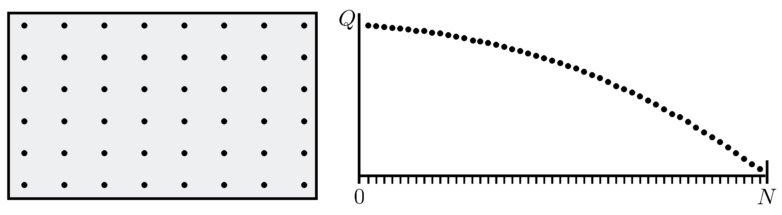
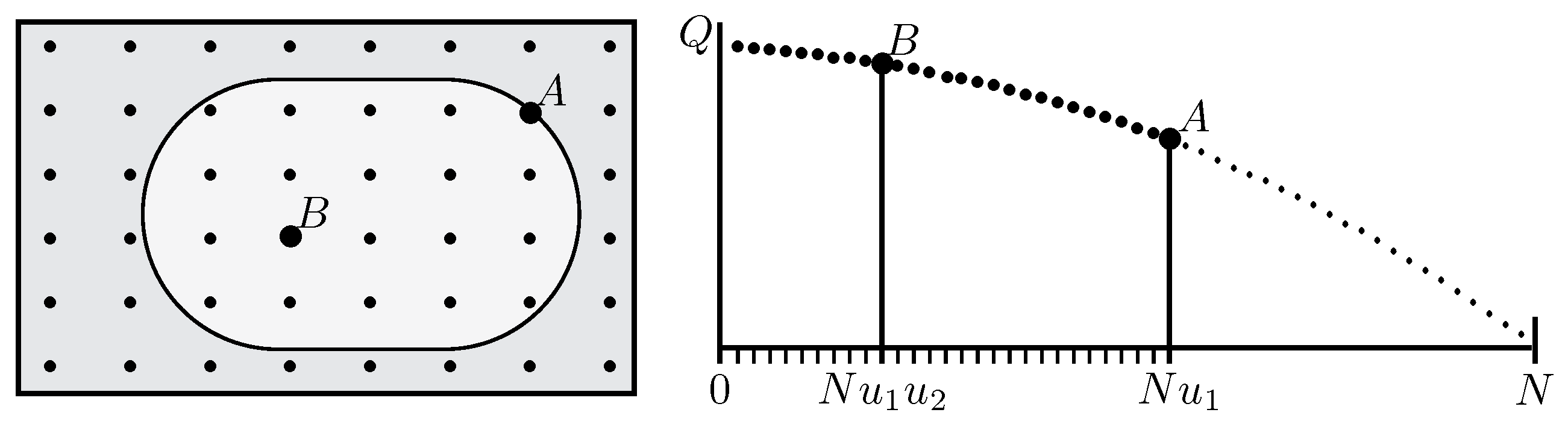
There may be very many (N) possible “locations” $\mathbf{x}$ to choose from. For clarity, assume these have equal status a priori—there is no loss of generality because unequal status can always be modelled by retreating to an appropriate substratum of equivalent points. For the avoidance of doubt, we are investigating practical computation so N is finite, though with no specific limit.

As the first step, the programmer with no initial guidance available can at best select a random location ${\mathbf{x}}_1$ for the first evaluation $Q_1=Q\left({\mathbf{x}}_1\right)$. The task of locating larger values of Q carries no assumption of geometry or even topology. Locations could be shuffled arbitrarily and the task would remain just the same. Accordingly, we are allowed to shuffle the locations into decreasing Q-order without changing the task (Figure 1). If ordering is ambiguous because different locations have equal quality, the ambiguity can be resolved by assigning each location its own (random) key-value to break the degeneracy.

Being chosen at random, ${\mathbf{x}}_1$’s shuffled rank $N{u}_1$ marks an equally random fraction of the ordered N locations. Our knowledge of $u_1$ is uniform: $u_1\sim \mathtt{Uniform}(0,1)$. We can encode this knowledge as one or (better) more samples that simulate what the position might actually have been. If the programmer deems a single simulation too crude and many too bothersome, the mean and standard deviation

$$log{u}_1=-1\pm 1$$

(1)

often suffice.

The next step is to discard the “wrong” points with $Q<Q_1$ and select a second location ${\mathbf{x}}_2$ randomly from the surviving $N{u}_1$ possibilities. Being similarly random, ${\mathbf{x}}_2$’s rank $N{u}_1{u}_2$ marks a random fraction of those $N{u}_1$, with $u_2\sim \mathtt{Uniform}(0,1)$ (Figure 2).

And so on. After k steps of increasing quality $Q_1<Q_2<\cdots <Q_k$, the net compression ratio $X_k=u_1{u}_2\cdots u_k$ can be simulated as several samples from

$$X_k\sim \underset{k}{\underbrace{\mathtt{Uniform}(\mathtt{0},\mathtt{1})·\mathtt{Uniform}(\mathtt{0},\mathtt{1})·\dots ·\mathtt{Uniform}(\mathtt{0},\mathtt{1})}}$$

(2)

to get results fully faithful to our knowledge or simply abbreviated as mean and standard deviation

$$log{X}_k=\underset{k}{\underbrace{(-1\pm 1)+(-1\pm 1)+\dots (-1\pm 1)}}=-k\pm \surd k$$

(3)

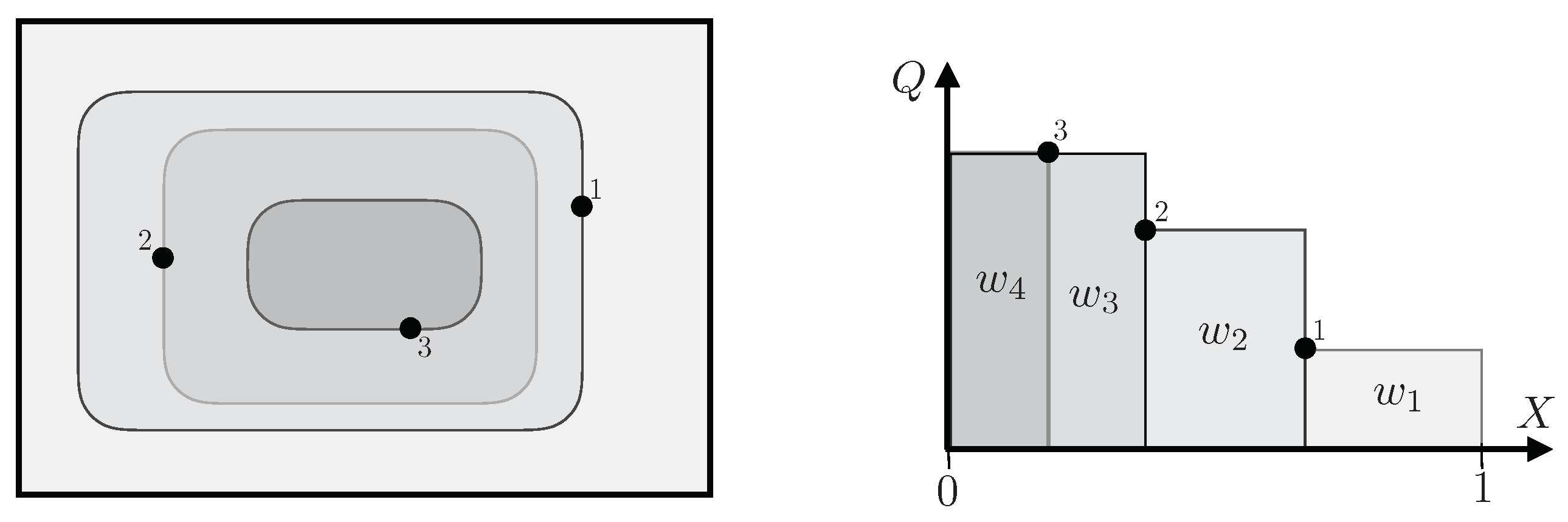
Compression proceeds exponentially until the user decides that Q has been adequately maximised. At that stage, the evaluated sequence $Q_1<Q_2<\cdots <Q_k$ of qualities Q has been paired with the corresponding sequence $X_1>X_2>\dots X_k$ of compressions X (Figure 3), either severally simulated or abbreviated in mean.

Q can then be integrated as

$$Z=\int Q\left(\mathbf{x}\right)d\mathbf{x}={\int }_0^{1}Q\left(X\right)dX\approx \sum _{i=1}^k{w}_i,w_i=Q_i\Delta X_i$$

(4)

so that quantification is available for Bayesian or other purposes. Any function of Q can be integrated too from the same run, changing $Q_i$ to some related $Q_i^{\prime }$ while leaving the $X_i$ fixed. And the statistical uncertainty in any integral Z is trivially acquired from the repeated simulations (2) of what the compressions X might have been according to their known distributions.

That’s nested sampling. It requires two user procedures additional to the $Q\left(\mathbf{x}\right)$ function. The first is to sample an initially random location to start the procedure. The second—which we next address—is to move to a new random location obeying a lower bound on Q. Note that there is no modulation within a constrained domain. Locations are either acceptable, $Q\left(\mathbf{x}\right)\ge Q^{*}$, or not, $Q\left(\mathbf{x}\right)<Q^{*}$.

3. Exploration by Galilean Monte Carlo

The obvious beginners’ MCMC procedure for moving from one acceptable location to another, while obeying detailed balance but not moving so far that Q always disobeys the lower bound $Q^{*}$, is:

$$\begin{gathered} \begin{array}{c}\mathtt{Start}\mathtt{at}\mathbf{x}\mathtt{with}\mathtt{acceptable}\mathtt{quality}Q\left(\mathbf{x}\right)\ge Q^{*}\hfill \\ \mathtt{Repeat}\mathtt{for}\mathtt{length}\mathtt{of}\mathtt{trajectory}\hfill \end{array} \\ \hspace{1em} \begin{array}{|c|}\hline \hfill \mathtt{Set}\mathbf{v}=\mathtt{isotropically}\mathtt{random}\mathtt{velocity}\hfill \\ \hfill {\mathbf{x}}^{\prime }=\mathbf{x}+\mathbf{v}=\mathtt{trial}\mathtt{location}\hfill \\ \mathrm{if} ( Q(\mathbf{x})\ge Q^{*} )\hfill & \mathtt{accept}\mathtt{new}\mathbf{x}=\mathbf{x}\prime \hfill \\ \mathtt{else}\hfill & \mathtt{reject}\mathbf{x}\prime \mathtt{by}\mathtt{keeping}\mathbf{x}\hfill \\ \hline\end{array} \end{gathered}$$

(5)

However, randomising $\mathbf{v}$ every step is diffusive and slow, with net distance travelled increasing only as the square root of the number of steps.

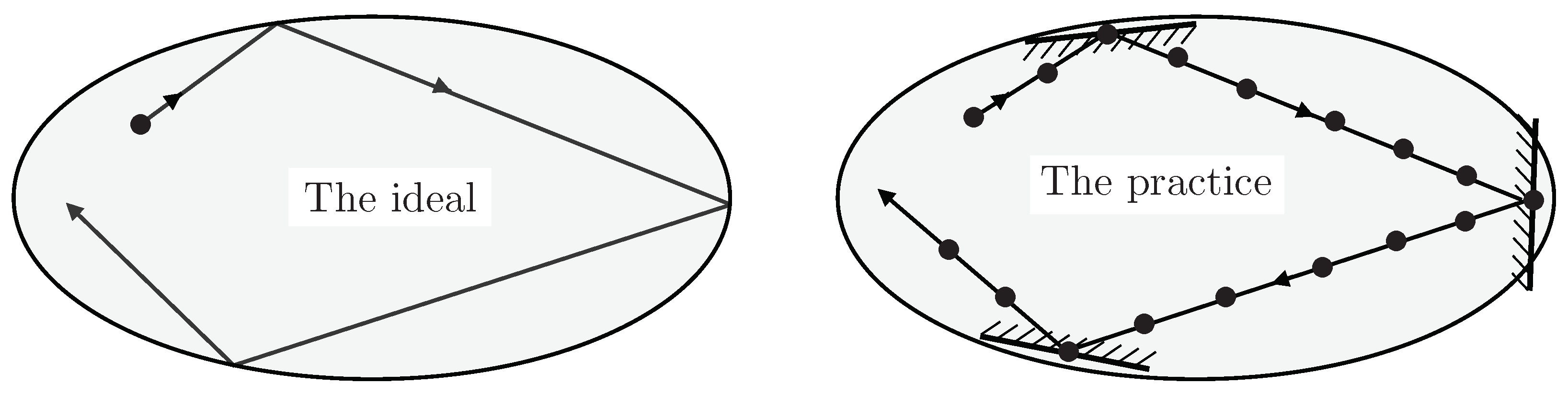
All locations within the constrained domain are equally acceptable, so the program might better try to proceed in a straight line, changing velocity only when necessary in an attempt to reflect specularly off the boundary (Figure 4, left). The user is asked to ensure that the imposed geometry makes sense in the context of the particular application, otherwise there will be no advantage.

With finite step lengths, it’s not generally possible to hit the boundary exactly whilst simultaneously being sure that it had not already been encountered earlier, so the ideal path is impractical. Instead, we take a current location $\mathbf{x}$ and suppose that a corresponding unit vector $\mathbf{n}$ can be defined there as a proxy for where the surface normal would be if that surface was close at hand (Figure 4, right). Again, it is the user’s responsibility to ensure that $\mathbf{n}$ makes sense in the context of the particular application: exploration procedures cannot anticipate the quirks of individual applications.

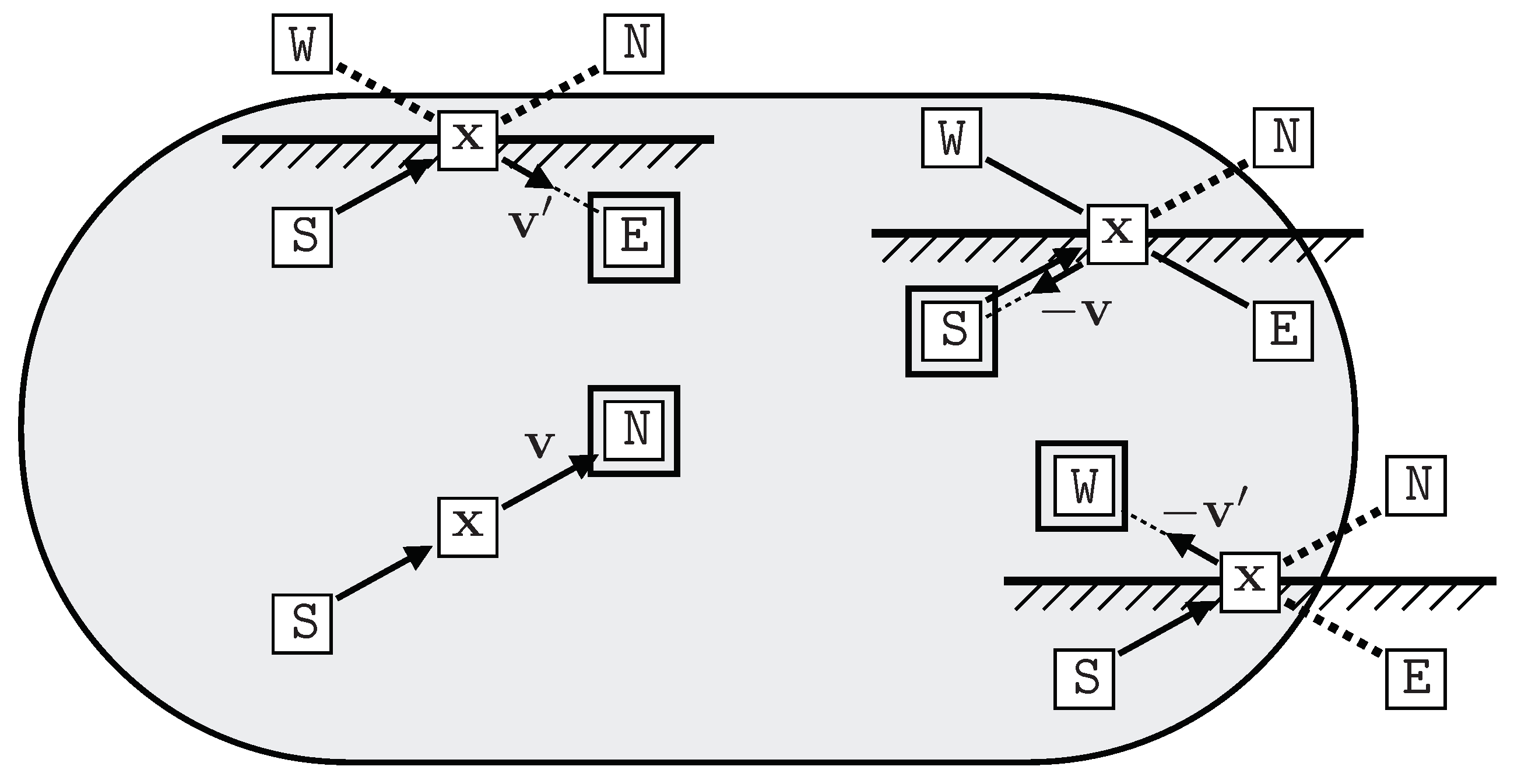
Reflection from a plane orthogonal to $\mathbf{n}$ (drawn horizontally in Figure 5) modifies an incoming velocity $\mathbf{v}$ (in northward direction from the South) to ${\mathbf{v}}^{\prime }=\mathbf{v}-2\mathbf{n}\left({\mathbf{n}}^T\mathbf{v}\right)$. Depending on the circumstances, the incoming particle may proceed straight on to the North ($+\mathbf{v}$), or be reflected to the East ($+{\mathbf{v}}^{\prime }$), or back-reflected to the West ($-{\mathbf{v}}^{\prime }$), or reversed back to the South ($-\mathbf{v}$).

• Mistakenly, the author’s earlier introduction of GMC in 2011 [4] reduced the possibilities by eliminating West, but at the cost of allowing the particle to escape the constraint temporarily, which damaged the performance and cancelled its potential superiority.

Figure 5. North – East – West – South, the four Galilean outcomes.

Figure 5. North – East – West – South, the four Galilean outcomes.

If the potential destination North is acceptable (bottom left in Figure 5), the particle should move there and not change its direction (so $\mathbf{n}$ need not be computed). Otherwise, the particle needs to change its direction but not its position.

For a North-South oriented velocity to divert into East-West, either East or West must be acceptable, but not both because East-West particles would then pass straight through without interacting with North-South, so the proposed diversion would break detailed balance. Likewise, for an East-West velocity to divert North-South, either North or South must be acceptable but not both. These conditions yield the following procedure:

$$\begin{gathered} \begin{array}{c}\mathtt{Start}\mathtt{at}\mathbf{x}\mathtt{with}\mathtt{acceptable}\mathtt{quality}Q\left(\mathbf{x}\right)\ge Q^{*}\hfill \\ \mathtt{Set}\mathbf{v}=\mathtt{isotropically}\mathtt{random}\mathtt{velocity}\hfill \\ \mathtt{Repeat}\mathtt{for}\mathtt{length}\mathtt{of}\mathtt{trajectory}\hfill \end{array} \\ \hspace{1em}\hspace{1em}\hspace{1em}\hspace{1em}\hspace{1em}\hspace{1em}\hspace{1em}\hspace{1em}\hspace{1em}\hspace{1em}\hspace{1em}\hspace{1em}\hspace{1em}\hspace{1em}\hspace{1em}\hspace{1em}\begin{array}{|c|}\hline \mathtt{Set}\mathtt{N}=“Q(\mathbf{x}+\mathbf{v})\ge Q^{*}”\hfill \\ \mathtt{if}( \mathtt{N} )\hfill & \mathtt{exit}\mathtt{with}\mathbf{x}=\mathbf{x}+\mathbf{v}\hfill & \left[\mathtt{go}\mathtt{North}\right]\hfill \\ \mathtt{Set}{\mathbf{v}}^{\prime }=\mathbf{Rv}=\mathtt{reflection}\mathtt{velocity}\hfill \\ \mathtt{Set}\mathtt{E}=“Q(\mathbf{x}+{\mathbf{v}}^{\prime })\ge Q^{*}”,\hfill & \mathtt{W}=“Q(\mathbf{x}-{\mathbf{v}}^{\prime })\ge Q^{*}”,\hfill & \mathtt{S}=“Q(\mathbf{x}-\mathbf{v})\ge Q^{*}”\hfill \\ \mathtt{if}( \mathtt{S} \mathtt{\&} (\mathtt{E}\mathtt{but}\mathtt{not}\mathtt{W}) )\hfill & \mathtt{exit}\mathtt{with}\mathbf{v}={\mathbf{v}}^{\prime }\hfill & \left[\mathtt{aim}\mathtt{East}\right]\hfill \\ \mathrm{if}( \mathtt{S} \mathtt{\&} (\mathtt{W}\mathtt{but}\mathtt{not}\mathtt{E}) )\hfill & \mathtt{exit}\mathtt{with}\mathbf{v}=-{\mathbf{v}}^{\prime }\hfill & \left[\mathtt{aim}\mathtt{West}\right]\hfill \\ \mathtt{otherwise}\hfill & \mathtt{exit}\mathtt{with}\mathbf{v}=-\mathbf{v}\hfill & \left[\mathtt{aim}\mathtt{South}\right]\hfill \\ \hline\end{array} \end{gathered}$$

(6)

Any self-inverse reflection operator $\mathbf{R}$ will do, though the reflection idea suggests $\mathbf{R}=\mathbf{I}-2\mathbf{n}{\mathbf{n}}^T$.

That’s Galilean Monte Carlo. The trajectory is explored uniformly, with each step yielding an acceptable (though correlated) sample.

4. Compression and Exploration

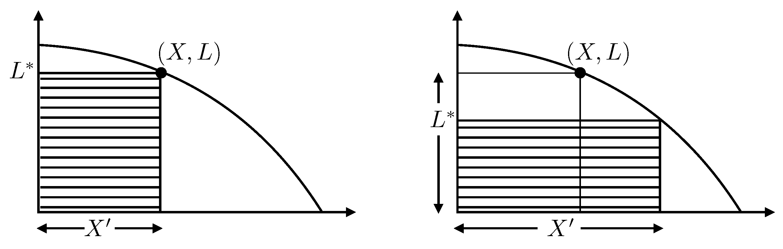
GMC was originally designed for nested-sampling compression, from which probability distributions can be built up after a run by identifying quality as likelihood L in the weighted sequence (4) of successively compressed locations. However, GMC can also be used when exploring a weighted distribution directly.

For compression (standard nested sampling, Figure 6, left), only the domain size X is iterated, albeit under likelihood control.

$$\begin{array}{cc}Compression:& \begin{array}{|c|}\hline \mathtt{Enter}\mathtt{with}X\mathtt{and}L\hfill \\ \mathtt{Set}\mathtt{constraint}{L}^{*}=L\mathtt{defining}{X}^{*}\hfill \\ \mathtt{Sample}\mathtt{within}{L}^{*}\mathtt{to}\mathtt{get}{X}^{\prime }=u{X}^{*}\hfill \\ \mathtt{Exit}\mathtt{with}{X}^{\prime }\mathtt{and}{L}^{\prime }\hfill \\ \hline\end{array}\end{array}$$

(7)

For exploration (standard reversible MCMC, Figure 6, right), the likelihood is relaxed as well through a preliminary random number $u^{\prime }\sim \mathtt{Uniform}(0,1)$.

$$\begin{array}{cc}Exploration:& \begin{array}{|c|}\hline \mathtt{Enter}\mathtt{with}X\mathtt{and}L\hfill \\ \mathtt{Set}\mathtt{constraint}{L}^{*}=u^{\prime }L\mathtt{defining}{X}^{*}\hfill \\ \mathtt{Sample}\mathtt{within}{L}^{*}\mathtt{to}\mathtt{get}{X}^{\prime }=u{X}^{*}\hfill \\ \mathtt{Exit}\mathtt{with}{X}^{\prime }\mathtt{and}{L}^{\prime }\hfill \\ \hline\end{array}\end{array}$$

(8)

This is equivalent to standard Metropolis balancing “Accept ${\mathbf{x}}^{\prime }$ if $L\left({\mathbf{x}}^{\prime }\right)\ge u^{\prime }L\left(\mathbf{x}\right)$”, the only difference being that the lower bound $u^{\prime }L$ is set beforehand instead of checked afterwards.

5. Exploration by Hamiltonian Monte Carlo

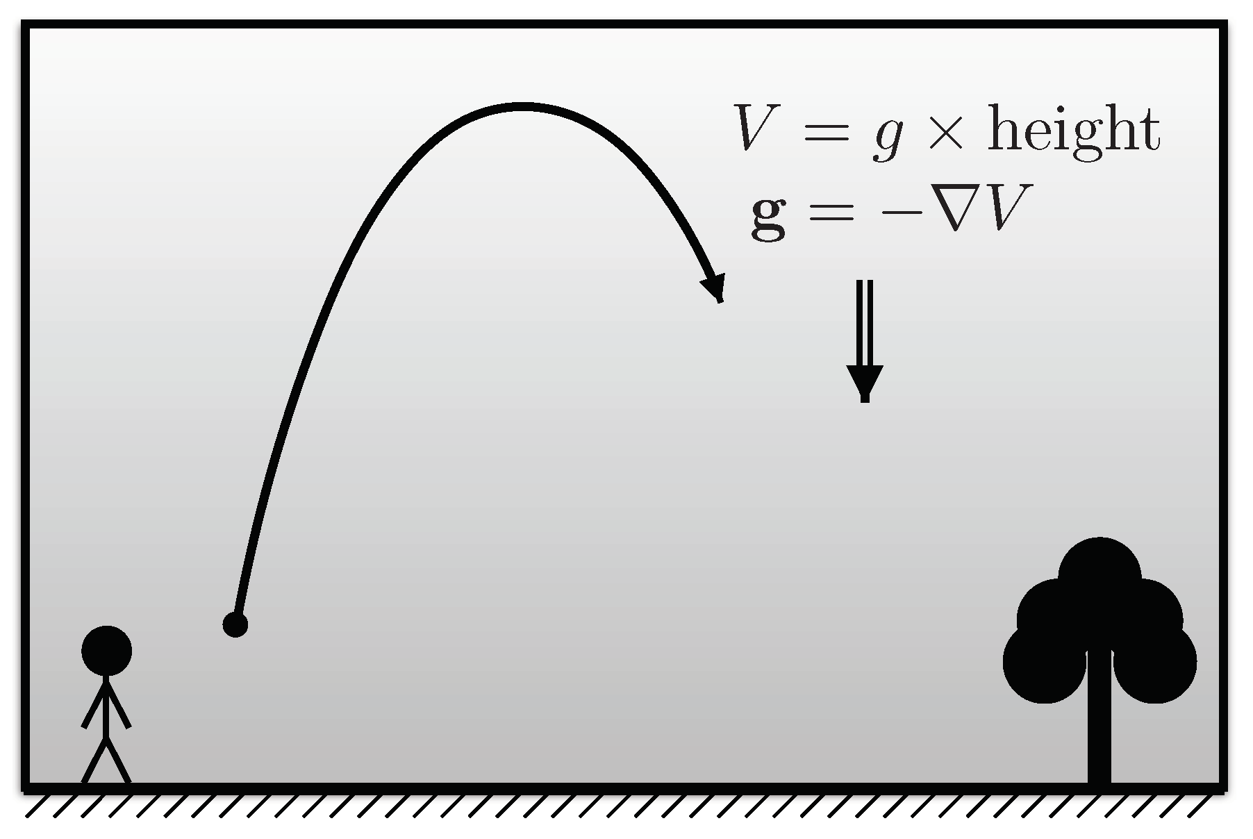
Hamiltonian Monte Carlo (HMC) [3] uses a physical analogy with kinetic theory of gases in which a thermal distribution of moving particles, whose position/velocity probability distribution factorises into space and velocity parts

$$Pr(\mathbf{x},\mathbf{v})\propto e^{-E(\mathbf{x},\mathbf{v})},E(\mathbf{x},\mathbf{v})=V\left(\mathbf{x}\right)+T\left(\mathbf{v}\right)$$

(9)

with potential energy V defining the spatial target distribution $Pr\left(\mathbf{x}\right)\propto e^{-V\left(\mathbf{x}\right)}$ and kinetic energy $T=\frac{1}{2}{\left|\mathbf{v}\right|}^2$ distributed as the Boltzmann thermal equilibrium $Pr\left(\mathbf{v}\right)\propto e^{-T\left(\mathbf{v}\right)}$.

The usual dynamics (Figure 7)

$$\frac{d\mathbf{x}}{dt}=\mathbf{v},\frac{d\mathbf{v}}{dt}=-\nabla V\left(\mathbf{x}\right)$$

(10)

relaxes an initial setting towards the joint equilibrium (9) under occasional collisions which reset $\mathbf{v}$ according to $Pr\left(\mathbf{v}\right)$, leaving $\mathbf{x}$ as a sample from the target $Pr\left(\mathbf{x}\right)$.

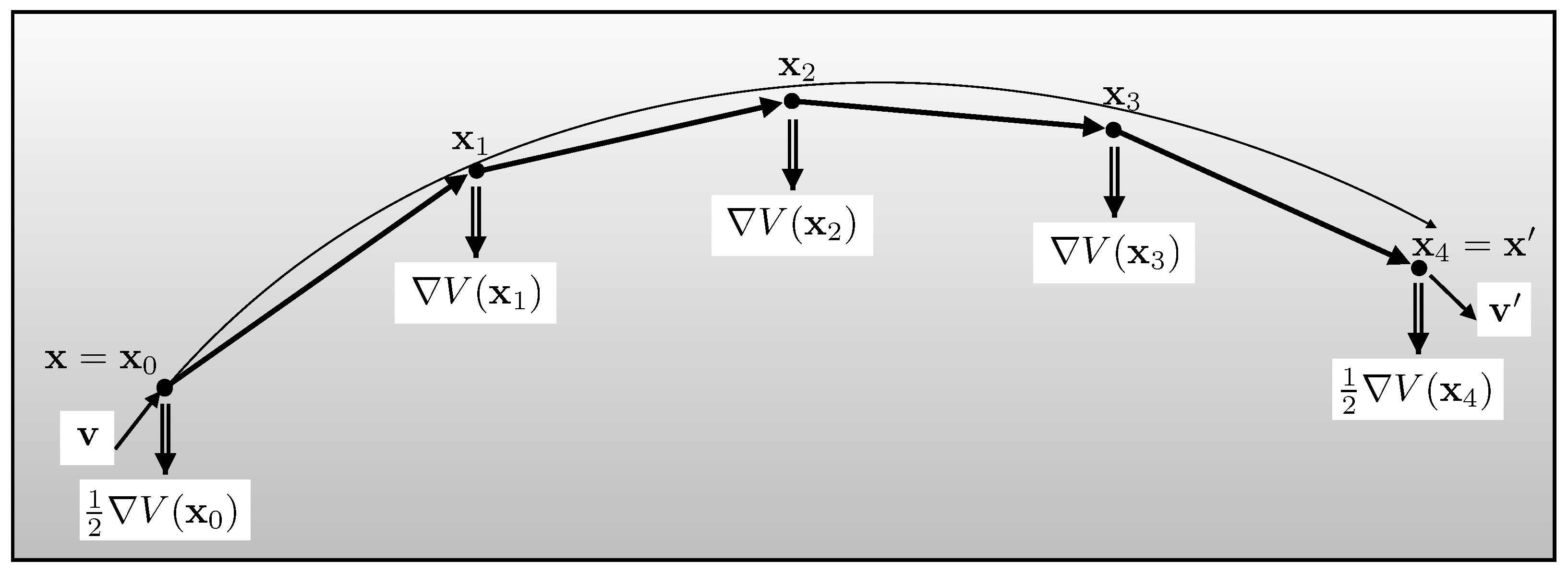
Between collisions, the force field is necessarily digitised into impulses at discrete time intervals $\delta t$, so the computation obeys

$$\delta \mathbf{x}=\mathbf{v}\delta t,\delta \mathbf{v}=-\nabla V\left(\mathbf{x}\right)\delta t$$

(11)

To make the trajectory reversible and increase the accuracy order, the impulses are halved at the start $\mathbf{x}$ and end ${\mathbf{x}}^{\prime }$, but even this does not ensure full accuracy because the dynamics has been approximated (Figure 8).

To correct this, the destination ${\mathbf{x}}^{\prime }$, whose total energy $E^{\prime }=V^{\prime }+T^{\prime }$ ought to agree with the initial $E=V+T$, is subjected to the usual Metropolis balancing.

$$\mathrm{Accept}{\mathbf{x}}^{\prime }\mathrm{iff}{e}^{-E^{\prime }}\ge e^{-E}·\mathtt{Uniform}(0,1).$$

(12)

In practice, the correction is often ignored because the (reversible) algorithm explores “level sets” whose contours are often an adequately good approximation to the true Hamiltonian provided the fixed timestep is not too large.

That’s Hamiltonian Monte Carlo. The trajectory is explored non-uniformly, with successive steps being closer at altitude where the particles are moving slower, so that sampling is closer where the density is smaller—a mismatch which needs to be overcome by the equilibrating collisions. And, of course, HMC requires the potential $V\left(\mathbf{x}\right)$ (a.k.a. log-likelihood) to be differentiable and generally smooth.

6. Compression versus Simulated Annealing

Simulated annealing uses a physical analogy to thermal equilibrium to compress from a prior probability distribution to a posterior. As in HMC, though without the complication of kinetic energy, the likelihood (or quality) is identified as the exponential $L=e^{-E}$ of an energy. In annealing, the energy is scaled by a parameter $\beta$ so that the quality becomes $Q=L^{\beta }=e^{-\beta E}$ of this scaled energy, with $\beta$ used to connect posterior (where $\beta =1$) with prior (where $\beta =0$).

This “simulates” thermal equilibrium at coolness (inverse temperature) $\beta$, and “annealing” refers to sufficiently gradual cooling from prior to posterior that equilibrium is locally preserved. A few lines of algebra, familiar in statistical mechanics, show that the evidence (or partition function) can be accumulated from successive thermal equilibria as

$$logZ={\int }_0^1{\langle logL\rangle }_{\beta }d\beta$$

(13)

where ${\langle logL\rangle }_{\beta }$ is the average log-likelihood as determined by sampling the equilibrium appropriate to coolness $\beta$. Equilibrium is defined by weights $L^{\beta }$ and can be explored either by GMC or (traditionally) by HMC. There is seldom any attempt to evaluate the statistical uncertainty in $logZ$, the necessary fluctuations being poorly defined in the simulations.

At coolness $\beta$, the equilibrium distribution of locations $\mathbf{x}$, initially uniform over the prior, is modulated by $L^{\beta }$ so that the samples have probability distribution $Pr\left(\mathbf{x}\right)\propto L{\left(\mathbf{x}\right)}^{\beta }$ which corresponds to

$$Pr\left(X\right)\propto L{\left(X\right)}^{\beta }$$

(14)

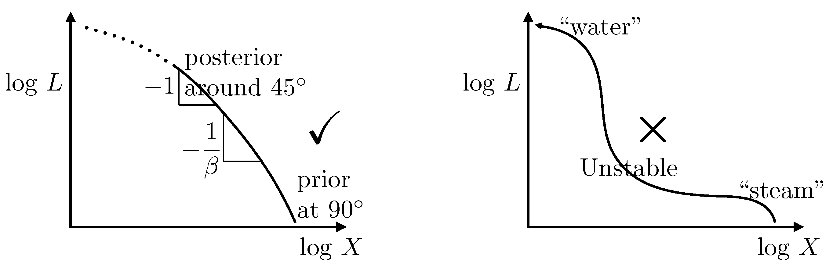
in terms of compression. Consequently, samples cluster around the maximum of $\beta logL+logX$, where the $logL(logX)$ curve has slope $-1/\beta$ (Figure 9, left). Clearly this only works properly if $logL(logX)$ is concave ($\stackrel{⌢}{}$). Any zone of convexity ($\stackrel{⌣}{}$) is unstable, with samples heading toward either larger L at little cost to X or toward larger X at little cost to L. A simulated-annealing program cannot enter a convex region, and the steady cooling assumed in (13) cannot occur.

In the physics analogy, this behaviour is a phase change and can be exemplified by the transition from steam to water at 100 °C (Figure 9, right). Because of the different volumes (exponentially different in large problems), a simulated-annealing program will be unable to place the two phases in algorithmic contact, so will be unable to model the latent heat of the transition. Correspondingly, computation of evidence Z will fail. Yet our world is full of interesting phase changes, and a method that cannot cope with them cannot be recommended for general use.

Nested sampling, on the other hand, compresses steadily with respect to the abscissa $logX$ regardless of the (monotonic) behaviour of $logL$, so is impervious to this sort of phase change. Contrariwise, simulated annealing cools through the slope, which need not change monotonically. By using thermal equilibria which average over $e^{-\beta E}$, simulated annealing views the system through the lens of a Laplace transform, which is notorious for its ill-conditioning. Far better to deal with the direct situation.

7. Conclusions

The author suggests that, just as nested sampling dominates simulated annealing, …

Nested sampling	Simulated Annealing
Steady compression	Arbitrary cooling schedule for $\beta$
Invariant to relabelling Q	Q has fixed form $L^{\beta }$
Can deal with phase changes	Cannot deal with phase changes
Evidence $Z=\int LdX$ with uncertainty	Evidence $Z=exp{\int }_0^1{\langle logL\rangle }_{\beta }d\beta$

… so does Galilean Monte Carlo dominate Hamiltonian.

Galilean Monte Carlo	Hamiltonian Monte Carlo
No rejection	Trajectories can be rejected
Any metric is OK	Riemannian metric required
Invariant to relabelling Q	Trajectory explores nonuniformly
Quality function $Q\left(\mathbf{x}\right)$ is arbitrary	Quality $Q\left(\mathbf{x}\right)$ must be differentiable
Step functions OK (nested sampling)	Can not use step functions
Can sample any probability distribution	Probability distribution must be smooth
Needs 2 work vectors	Needs 3 work vectors

In each case, reverting to elementary principles by discarding physical analogies enhances generality and power.