Proceeding Paper

A Sequential Marginal Likelihood Approximation Using Stochastic Gradients †

1
Department of Physics, Stellenbosch University, Stellenbosch 7600, South Africa
2
National Institute for Theoretical Physics, Stellenbosch 7600, South Africa
3
Computer Science Division, Stellenbosch University, Stellenbosch 7600, South Africa
*
Author to whom correspondence should be addressed.
Presented at the 39th International Workshop on Bayesian Inference and Maximum Entropy Methods in Science and Engineering, Garching, Germany, 30 June–5 July 2019.
Proceedings 2019, 33(1), 18; https://doi.org/10.3390/proceedings2019033018
Published: 3 December 2019

Abstract

:
Existing algorithms like nested sampling and annealed importance sampling are able to produce accurate estimates of the marginal likelihood of a model, but tend to scale poorly to large data sets. This is because these algorithms need to recalculate the log-likelihood for each iteration by summing over the whole data set. Efficient scaling to large data sets requires that algorithms only visit small subsets (mini-batches) of data on each iteration. To this end, we estimate the marginal likelihood via a sequential decomposition into a product of predictive distributions p ( y n | y < n ) . Predictive distributions can be approximated efficiently through Bayesian updating using stochastic gradient Hamiltonian Monte Carlo, which approximates likelihood gradients using mini-batches. Since each data point typically contains little information compared to the whole data set, the convergence to each successive posterior only requires a short burn-in phase. This approach can be viewed as a special case of sequential Monte Carlo (SMC) with a single particle, but differs from typical SMC methods in that it uses stochastic gradients. We illustrate how this approach scales favourably to large data sets with some simple models.

1. Introduction

Marginal likelihood (ML), sometimes call evidence, is a quantitative measure of how well a model can describe a particular data set; it is the probability that the data set occurred within that model. Consider a Bayesian model with parameters θ for a data set D = { y n } n = 1 N . The ML is the integral
Z : = p ( D ) = p ( D | θ ) p ( θ ) d θ ,
where p ( D | θ ) is the likelihood and p ( θ ) is the prior. In this paper we consider the case where the data are conditionally independent given the parameters
p ( D | θ ) = n p ( y n | θ ) ,
as is common in many parametric models. The posterior distribution over a set of models is proportional to their ML and so approximations to it are sometimes used for model comparison, and weighted model averaging [1] (chapter 12). This integral is typically analytically intractable for any but the simplest models, so one must resort to numerical approximation methods. Nested sampling (NS) [2] and annealed importance sampling (AIS) [3] are two algorithms able to produce accurate estimates of the ML. NS accomplishes this by sampling from the prior under constraints of increasing likelihood, and AIS by sampling from a temperature annealed distribution p ( D | θ ) β p ( θ ) and averaging over samples with appropriately calculated importance weights. Although NS and AIS produce accurate estimates of the ML, they tend to scale poorly to large data sets due the fact that they need to repeatedly calculate the likelihood function: for NS this is to ensure staying within the constrained likelihood contour; for AIS the likelihood must be calculated both to sample from the annealed distributions using some Markov chain Monte Carlo (MCMC) method, as well as to calculate the importance weights. Calculation of the likelihood is computationally expensive on large data sets. To combat this problem, various optimization and sampling algorithms rather make use of stochastic approximations of the likelihood by sub-sampling the data set into mini-batches B D [4]. The stochastic log-likelihood approximation is
log p ( D | θ ) | D | | B | y B log p ( y | θ ) ,
with each iteration of these algorithms generally using a different mini-batch. Unfortunately NS and AIS cannot trivially use mini-batching to improve scalability. Using stochastic likelihood approximations changes the statistics of the likelihood contours in NS, allowing particles to occasionally move to lower likelihood instead of higher, violating the basic assumptions of the algorithm. AIS could benefit from using stochastic likelihood gradients during the MCMC steps, but it is not obvious how one would calculate the importance weights in this setting. This work presents an approach for large-scale ML approximations using mini-batches. This is done using a sequential decomposition of the ML into predictive distributions, which can each be approximated using stochastic gradient MCMC methods. The particles sampled from each previous posterior distribution can be reused for efficiency since they will typically be close to the next posterior. This can be viewed as a special case of sequential Monte Carlo with Bayesian updating [5].
We illustrate our approach by calculating ML estimates on three simple models. For these models, we obtain roughly an order of magnitude speedup over nested sampling on data sets with one million observations with negligible loss in accuracy.

2. Sequential Marginal Likelihood Estimation

The ML can be decomposed, through the product rule, into a product of predictive distributions of the following form
Z = n p ( y n | y < n ) ,
where, from Equation (1),
p ( y n | y < n ) = p ( y n | θ ) p ( θ | y < n ) d θ .
Assuming one is able to produce accurate estimates p ^ ( y n | y < n ) of the predictive probabilities, the log-ML can be approximated by
log Z ^ = n log p ^ ( y n | y < n ) .
In this way the difficult problem of estimating an integral of an extremely peaked function, p ( D | θ ) , reduces to the easier problem of estimating many integrals of smoother functions p ( y n | θ ) . Note that this approach can more generally be applied using any other sequential decomposition of the data set. We only present derivations using the approach above for notational clarity but we decompose the data into varying-sized chunks of observations during our experiments as discussed in Section 4.
Typical sequential Monte Carlo (SMC) methods use a similar approach, and calculate predictive estimates using a combination of importance resampling and MCMC mutation steps [5]. Generic examples of such algorithms are the bootstrap particle filter [6], which is often used for posterior inference in hidden Markov models and other latent variable sequence models [5], and the “left-to-right” algorithm which is used in [7] to evaluate topic models.
The computational efficiency of using this approach depends on the method of approximating Equation (2). One such estimator is
p ^ ( y n | y < n ) = 1 M i = 1 M p ( y n | θ i ) ,
where each θ i is drawn from the posterior distribution p ( θ | y < n ) using MCMC methods. Again, one might use a chunk of observations for this predictive estimate rather than just one. As described in [8], estimators of this form tend to underestimate the ML, but still converge to the exact ML in the limit M . Since samples from the previous posterior, p ( θ | y < n 1 ) , would generally be available at each step, we expect only a small number of steps will be needed to accurately sample from the next posterior distribution, p ( θ | y < n ) . Metropolis-Hastings based MCMC algorithms would have to iterate over the previous n 1 data points in order to calculate the acceptance probability for each Markov transition, and so using them to estimate log Z in this sequential manner would scale at least quadratically in N. The key computational improvement in our approach is instead using stochastic gradient based MCMC algorithms such as stochastic gradient Hamiltonian Monte Carlo [9]. SGHMC utilizes mini-batching, allowing one to efficiently draw samples from the posterior distribution p ( θ | y < n ) even when n is large. We now describe how one can use SGHMC to sample from posterior distributions.

3. Stochastic Gradient Hamiltonian Monte Carlo

SGHMC [9] simulates a Brownian particle in a potential, by numerically integrating the Langevin equation
d θ = v d t d v = U ( θ ) d t γ v d t + 2 γ d W ,
where U ( θ ) is the potential energy, γ is the friction coefficient and W is the standard Wiener process [10]. That is, each increment Δ W is independently normally distributed with mean zero and variance Δ t . It can be shown through the use of a Fokker-Planck equation [11], that the above dynamics converge to the stationary distribution
p ( θ , v ) exp U ( θ ) v 2 2 .
We can use this to sample from the full data posterior by using a potential energy equal to the negative log-joint U ( θ ) : = log p ( D , θ ) . The numeric integration is typically discretized [9,12] as follows
Δ θ = v Δ v = η U ^ ( θ ) α v + ϵ 2 ( α β ^ ) η ,
where η is called the learning rate, 1 α is the momentum decay, ϵ is a standard Gaussian random vector, β ^ is an optional parameter to offset the variance of the stochastic gradient term and
U ^ ( θ ) = | D | | B | y B log p ( y | θ ) log p ( θ )
is an unbiased estimate of U ( θ ) . A new mini-batch B is sampled for each iteration of Equation (5). Since U ( θ ) grows with the size of the data set, a small learning rate η O ( 1 | D | ) is required to minimize the discretization error. The variance of the stochastic gradient term is proportional to η 2 while the variance of the injected noise is proportional to η , so in the limit η 0 , stochasticity in the gradient estimates becomes negligible and the correct continuum dynamics are recovered, even if one ignores the errors from the stochastic gradient noise and β ^ = 0 is used. We refer the reader to [9,13,14] for an in-depth analysis of the algorithm parameters.
For the purposes of Bayesian updating, we use SGHMC to sample from the nth posterior distribution, p ( θ | y n ) , using the stochastic potential energy
U ^ n ( θ ) = n 1 | B | y B log p ( y | θ ) log p ( y n | θ ) log p ( θ ) ,
where the mini-batch is drawn i.i.d. with replacement from the set of all previous data points i.e., B { y k | k < n } . The extra term here is to ensure that the previously unseen data point is always taken into account. If the extra term was not included, there would be some chance that the new data point does not get taken into account during the SGHMC steps. With this potential energy SGHMC still converges to the required posterior distribution, since it is still an unbiased estimator of the negative log-joint.

4. Experiments

We use mini-batches of size 500, with the following SGHMC parameters: η = 0.1/ n , α = 0.2 and β ^ = 0 . Predictive distributions are approximated using M = 10 samples and 20 burn-in steps for each new posterior. As mentioned in Section 2, rather than Bayesian updating by adding a single observation at a time, we add chunks of data at a time. In the following experiments we use chunks of 20 data points when n 80 , chunks of size n 4 when 80 < n < 2000 , and chunks of size 500 thereafter. Our motivation for this is because we expect that smaller chunk sizes will give a lower variance in the estimator Equation (4) when n is small and so the posterior is less peaked, but for large n using larger chunk sizes is more efficient.
We use NS as our reference standard of accuracy. We implement NS with 20 SGHMC steps to sample from the constrained prior. For SGHMC used with NS we used parameters η = 10 3 , α = 0.1 and β ^ = 0 because there is no gradient noise when sampling from the prior. Results reported are for two particles; more behave similarly but are slower. We allow NS to run until the additive terms are less than 1% of the current Z ^ estimate. This is a popular stopping criterion and is also used in [8]. For more information on the constrained sampler and NS see Appendix A. Our experiments were run on a laptop with an Intel i7 CPU. For fair comparison, all code is single threaded. Multithreading gives a considerable speedup when calculating the likelihood on large data sets but can introduce subtle complexities that are difficult to control for in tests of runtime performance.
We evaluate our approach on the following three models using simulated data sets:

4.1. Linear Regression

The data set consists of pairs ( x , y ) related by
y = w T x + b + ϵ ,
where ϵ is zero mean Gaussian distributed with known variance σ 2 . We do not assume any distribution over x as it always appears on the right hand side of the conditional.
p ( y | x , w , b ) = 1 2 π σ 2 exp ( y w T x b ) 2 2 σ 2
Parameters are w and b, with standard Gaussian priors. ML can be calculated analytically for this model. We used 5 dimensional vectors x ; this model has 6 parameters.

4.2. Logistic Regression

The data set consists of pairs ( x , y ) , where x is an observation vector which is assigned a class label y { 1 , , K } . The labels have a discrete distribution with probabilities given by
p ( y | x , θ ) = exp ( w y T x + b y ) k exp ( w k T x + b k ) .
Parameters are θ = ( w 1 : K , b 1 : K ) , with standard Gaussian priors. Again we do not assume any distribution over x as it always appears on the right hand side of the conditional. We used 10 dimensional vectors x with 4 classes; this model has 44 parameters.

4.3. Gaussian Mixture Model

The data are modeled by a mixture of multivariate Gaussian distributions with diagonal covariance matrices. Mixture weights, means and variances are treated as parameters. This type of model is often treated as a latent variable model, where the mixture component assignments of each data point are the latent variables. Here we marginalize out the latent variables to obtain the following conditional distribution:
p ( y | θ ) = k = 1 K β k j = 1 d 1 2 π σ k , j 2 exp ( y j μ k , j ) 2 2 σ k , j 2 ,
θ = ( β 1 : K , μ 1 : K , 1 : d , σ 1 : K , 1 : d 2 ) .
Mixture weights β 1 : K are modeled by a Dirichlet prior with α = 1 ; means μ k , j are modeled by Gaussian priors, centered around zero and with variance 4 σ k , j 2 ; variances σ k , j 2 are modeled by inverse gamma priors with shape and scale parameters equal to 1. We used 5 Gaussian components and observations were 2 dimensional; this model has 25 parameters with 24 degrees of freedom.

5. Results and Discussion

The log-ML typically grows linearly in the number of data points. For this reason, it is natural to measure errors in log Z N rather than log Z . In [8], the authors suggest that errors in log Z N of 0.1 are acceptable. For each model, we measured the runtime performance of nested sampling and our sequential estimator for various data set sizes up to one million data points. Due to computational constraints we run NS only for data set sizes at logarithmically increasing intervals, while the sequential sampler naturally produces many more intermediate results in a single run. In some of the figures below, the sequential sampler initially underestimates the log-ML. We believe this is due to higher variance of Equation (4) when n is small, and so we also give a hybrid result which replaces the initial terms in Equation (3) with a NS estimate of the ML for the first 100 data points.

5.1. Linear Regression

For the linear regression model, the exact ML is available analytically and is shown in Figure 1a for comparison. Both algorithms are able to produce accurate results for this model for all data set sizes. The final error of the sequential sampler on one million data points is only about 10 4 N (roughly 0.01%). For this model, our method was faster than NS by about a factor of 3 on one million observations.

5.2. Logistic Regression

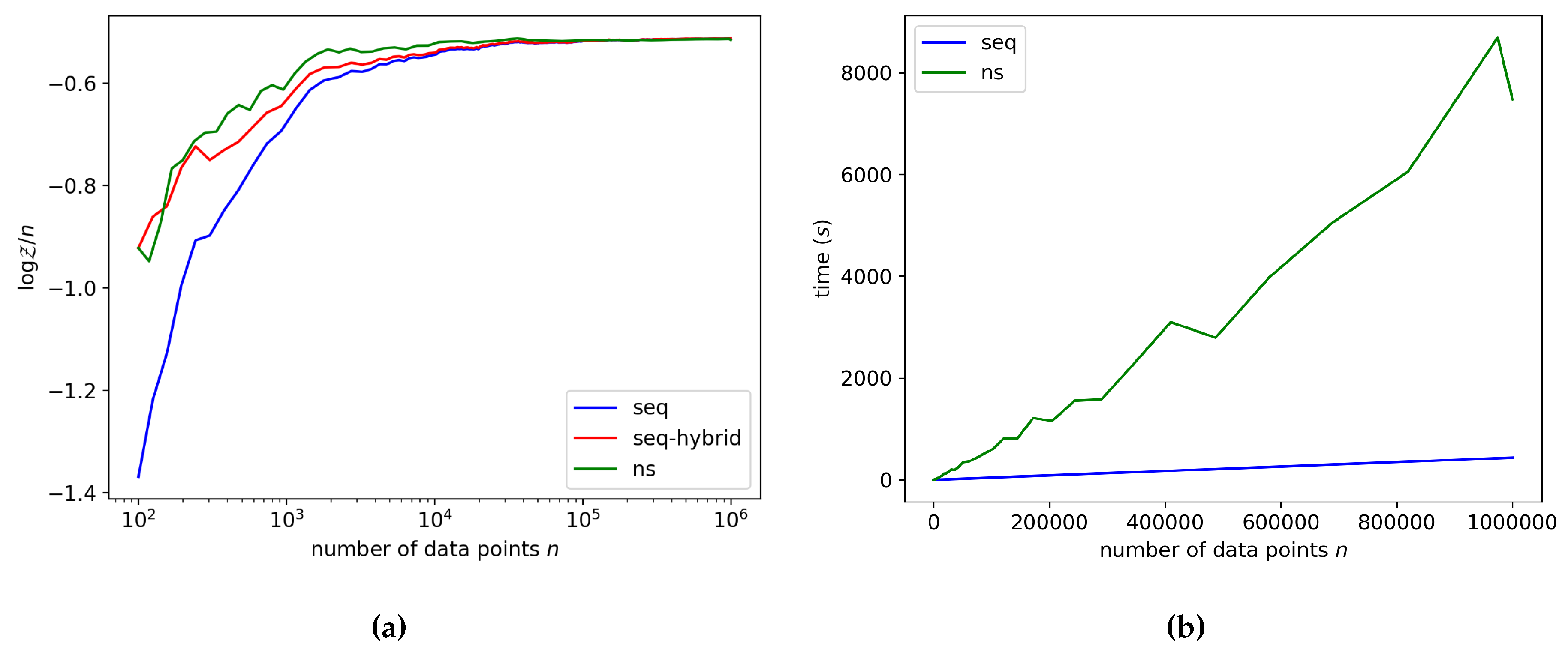
For the largest data set, NS and our sequential sampler produced estimates which differed by 3 × 10 4 N (roughly 0.7%), which is negligible. Our sequential sampler was almost a factor 17 faster than the nested sampler on one million observations for this model.

5.3. Gaussian Mixture Model

The posterior distribution for this model is multimodal. Some modes are due to permutation symmetries; these modes do not have to be explored since each one contains the same information. There are also some local modes which do not necessarily capture meaningful information about the data; for example, fitting a single Gaussian to the whole data set may be a poor local optimum of the likelihood function. If an MCMC walker finds one of these modes it can get trapped. However, we find that by Bayesian updating, the MCMC walkers tend to leave the poor local modes early on, before they become extremely peaked. This is similar to how annealing can help prevent MCMC and optimization algorithms from getting trapped in poor local optima. The estimates produced by NS and our sequential sampler differed on the largest data set by 2 × 10 3 N (roughly 0.06%). For this model our sequential sampler was about a factor 11 faster than the nested sampler on one million observations.
In all the experiments our sequential sampler seems to converge to the same result as NS within a negligible error for large n. The initial disagreement between NS and our sequential sampler on the first few thousand data points, seen in Figure 2a and Figure 3a, seems as if it can be attributed to the initial terms in Equation (3), since the proposed hybrid approach, replacing early terms in the sequential sampler by estimates based on NS, matches NS closely for all data set sizes.

6. Materials and Methods

Code for this work was implemented using pytorch [15]. The code for our experiments is available at https://gitlab.com/pleased/sequential-evidence.

7. Conclusions

We found that our sequential sampler using stochastic gradients was able to produce accurate ML estimates with a speedup over NS. Furthermore, since the marginal cost of updating the ML estimates when new data arrives does not depend on the number of previous data points, this approach may be effective for weighted model averaging in a setting where one periodically gets access to new data, such as in streaming applications. Potential future work may involve a more in-depth analysis of the algorithm parameters, for example automatic tuning of the number of samples, M, used for approximating predictive probabilities. One can imagine further exploring the effects of stochastic gradients for ML calculation in the full SMC setting, including latent variable models and resampling steps, with more general stochastic gradient MCMC algorithms such as those in [13].

Author Contributions

Conceptualization, methodology, software, formal analysis, investigation, visualization, writing–original draft preparation: S.A.C.; validation, writing–review and editing: S.A.C., H.C.E. and S.K.; resources: S.K.; project administration, supervision: H.C.E. and S.K.; funding acquisition: H.C.E.

Funding

S. Cameron received bursary support from the South African National Institute of Theoretical Physics, as well as financial support from both the organizers of MaxEnt 2019 and the National Institute of Theoretical Physics in attending the conference.

Acknowledgments

We wish to thank the organizers of MaxEnt 2019 and the South African National Institute of Theoretical Physics for financial support in attending the conference.

Conflicts of Interest

The authors declare no conflict of interest.

Abbreviations

The following abbreviations are used in this manuscript:
AISAnnealed importance sampling
MCMCMarkov chain Monte Carlo
MLMarginal likelihood
NSNested sampling
SGHMCStochastic gradient Hamiltonian Monte Carlo

Appendix A

Nested sampling requires one to sample from the prior under increasing likelihood constraints. Sampling under constraints is, in general, a difficult problem. This sampling can be accomplished by repeatedly sampling from the prior until the constraint is satisfied. This method of rejection sampling scales extremely poorly with both the size of the data set and the dimension of the parameter space, and is not feasible on any but the smallest problems. However NS using this rejection sampling method is a theoretically perfect implementation of NS, as it satisfies the assumptions of perfect i.i.d. sampling upon which NS is based. Further more it is extremely easy to implement correctly and so is a useful tool for testing the correctness of other NS implementation.
Our implementation of NS is based on SGHMC, simply because the code for SGHMC was already written. In order to sample under constraints we use a similar strategy to Galilean Monte Carlo as described in [16], where the particle reflects off of the boundary of the likelihood contour by updating the momentum as follows:
Δ v = 2 n ( v · n ) .
Here n is a unit vector parallel to the likelihood gradient θ p ( D | θ ) . While it is not the focus of our paper, we note that we have not previously encountered the idea of applying SGHMC to sampling under constraints; our implementation allows a fairly direct approach to implementing NS in a variety of contexts, and the technique may also potentially be of value in other constrained sampling contexts.
We found that, due to discretization error, the constrained sampler tends to undersample slightly at the boundaries of the constrained region; however the undersampled volume is of the order of the learning rate η and so can be neglected if a small enough learning rate is used.
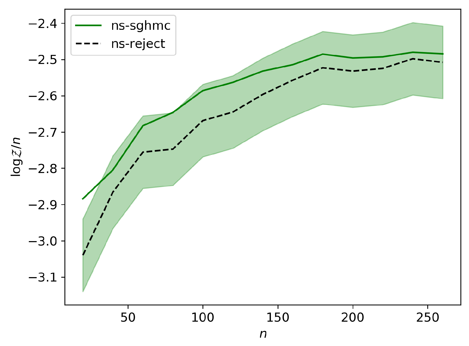
We tested the correctness of our constrained sampler against NS with rejection sampling for up to 250 observations. We found that the slight undersampling at the constraint boundaries tends to make the NS estimate slightly higher that that of the rejection sampler—see Figure A1—but the difference was within the acceptable range of 0.1N , and appears to be decreasing with the number of observations.
Figure A1. Comparison of NS with SGHMC to NS with rejection sampling for a 1-dimensional Gaussian mixture model with 9 parameters (8 degrees of freedom). The size of the shaded band is ± 0.1N around the rejection sampling implementation.
Proceedings 33 00018 g0a1

References

  1. Barber, D. Bayesian Reasoning and Machine Learning; Cambridge University Press: New York, NY, USA, 2012. [Google Scholar]
  2. Skilling, J. Nested sampling for general Bayesian computation. Bayesian Anal. 2006, 1, 833–859, doi:10.1214/06-BA127. [Google Scholar] [CrossRef]
  3. Neal, R.M. Annealed Importance Sampling. arXiv 1998, arXiv:physics/9803008. [Google Scholar]
  4. Welling, M.; Teh, Y.W. Bayesian Learning via Stochastic Gradient Langevin Dynamics. In Proceedings of the 28th International Conference on Machine Learning, ICML 2011, Bellevue, WA, USA, 28 June–2 July 2011; Getoor, L., Scheffer, T., Eds.; Omnipress: Madison, WI, USA, 2011; pp. 681–688. [Google Scholar]
  5. Naesseth, C.A.; Lindsten, F.; Schön, T.B. Elements of Sequential Monte Carlo. arXiv 2019, arXiv:1903.04797. [Google Scholar]
  6. Gordon, N.J.; Salmond, D.J.; Smith, A.F.M. Novel approach to nonlinear/non-Gaussian Bayesian state estimation. IEE Proc. F Radar Signal Process. 1993, 140, 107–113, doi:10.1049/ip-f-2.1993.0015. [Google Scholar] [CrossRef]
  7. Wallach, H.M.; Murray, I.; Salakhutdinov, R.; Mimno, D. Evaluation Methods for Topic Models. In Proceedings of the 26th Annual International Conference on Machine Learning, Montreal, QC, Canada, 14–18 June 2009; ACM: New York, NY, USA, 2009; pp. 1105–1112, doi:10.1145/1553374.1553515. [Google Scholar] [CrossRef]
  8. Grosse, R.B.; Ghahramani, Z.; Adams, R.P. Sandwiching the marginal likelihood using bidirectional Monte Carlo. arXiv 2015, arXiv:1511.02543. [Google Scholar]
  9. Chen, T.; Fox, E.; Guestrin, C. Stochastic Gradient Hamiltonian Monte Carlo. In Proceedings of the 31st International Conference on Machine Learning, Beijing, China, 21–26 June 2014; Volume 5. [Google Scholar]
  10. Durrett, R. Stochastic Calculus: A Practical Introduction; Probability and Stochastics Series; CRC Press: Boca Raton, FL, USA, 1996; pp. 177–207. [Google Scholar]
  11. Gardiner, C.W. Handbook of Stochastic Methods for Physics, Chemistry and the Natural Sciences, 3rd ed.; Volume 13, Springer Series in Synergetics; Springer: Berlin, Germany, 2004; p. xviii+415. [Google Scholar]
  12. Zhang, R.; Li, C.; Zhang, J.; Chen, C.; Wilson, A.G. Cyclical Stochastic Gradient MCMC for Bayesian Deep Learning. arXiv 2019, arXiv:1902.03932. [Google Scholar]
  13. Ma, Y.A.; Chen, T.; Fox, E.B. A Complete Recipe for Stochastic Gradient MCMC. arXiv 2015, arXiv:1506.04696. [Google Scholar]
  14. Springenberg, J.T.; Klein, A.; Falkner, S.; Hutter, F. Bayesian Optimization with Robust Bayesian Neural Networks. In Advances in Neural Information Processing Systems 29; Lee, D.D., Sugiyama, M., Luxburg, U.V., Guyon, I., Garnett, R., Eds.; Curran Associates, Inc.: Barcelona, Spain, 2016; pp. 4134–4142. [Google Scholar]
  15. Paszke, A.; Gross, S.; Chintala, S.; Chanan, G.; Yang, E.; DeVito, Z.; Lin, Z.; Desmaison, A.; Antiga, L.; Lerer, A. Automatic Differentiation in PyTorch. Available online: https://openreview.net/pdJsrmfCZ (accessed on 24 June 2019).
  16. Skilling, J. Bayesian Computation in Big Spaces-Nested Sampling and Galilean Monte Carlo. AIP Conf. Proc. 2012, 1443, 145–156, doi:10.1063/1.3703630. [Google Scholar] [CrossRef]
Figure 1. Linear regression model. (a) shows the accuracy of the sequential ML estimator compared to nested sampling and the exact ML and (b) shows the run time of both methods.
Proceedings 33 00018 g001
Figure 2. Logistic regression model. (a) shows the sequential ML estimator compared to nested sampling and (b) shows the run time of both methods.
Proceedings 33 00018 g002
Figure 3. Gaussian mixture model. (a) shows the sequential ML estimator compared to nested sampling and (b) shows the run time of both methods.
Proceedings 33 00018 g003