Low-Power Pedestrian Detection System on FPGA ^†

Abstract

Pedestrian detection is one of the key problems in the emerging self-driving car industry. In addition, the Histogram of Gradients (HOG) algorithm proved to provide good accuracy for pedestrian detection. Many research works focused on accelerating HOG algorithm on FPGA (Field-Programmable Gate Array) due to its low-power and high-throughput characteristics. In this paper, we present an energy-efficient HOG-based implementation for pedestrian detection system on a low-cost FPGA system-on-chip platform. The hardware accelerator implements the HOG computation and the Support Vector Machine classifier, the rest of the algorithm is mapped to software in the embedded processor. The hardware runs at 50 Mhz (lower frequency than previous works), thus achieving the best pixels processed per clock and the lower power design.

1. Introduction

Pedestrian detection is a safety-critical application on autonomous cars. There are two main approaches to implement pedestrian detection systems. On one hand, the detection algorithm relies on all input image pixels. This approach uses deep learning method and it requires costly computing platforms with not only many processing cores but also large memory bandwidth and capacity. On the other hand, only extracted features from the image will input the detection algorithm. This approach using HOG (Histogram of Gradients) [1] has proven to have good accuracy in detection [2]. While requiring less memory capacity, it is still a computing-intensive algorithm, which needs a low latency and high-throughput platform. FPGAs (Field-Programmable Gate Arrays), therefore, come as a suitable solution thanks to its capability in parallel processing. More importantly, FPGAs potentially have better energy efficiency in comparison with alternative platforms such as CPUs and GPUs. In this paper, we design and implement a pedestrian detection system, including a HOG feature extractor and an SVM classifier, on a low-cost FPGA device, targeting at high throughput and low power consumption. This work is an evolution of our previous works presented in [3,4]. There are several improvements to help achieving a high-performance design. First, the fixed-point number is used to represent values other than the integer number, which increases the feature’s accuracy with the cost of computational complexity. Secondly, a pipeline for normalizing cell features to take advantage of hardware’s capability in pipeline and parallel execution. Third, instead of buffering full input images, input pixels coming from the sensor use window pipelines before its processing. Fourth, an SVM classifier is implemented using FPGA’s programmable logic to further accelerating the detection system. Finally, we optimize the pipeline design to increase the number of frames processed per second. The throughput plays an important role in an energy-efficient design. The detection system works at a clock frequency of 50 MHz with a throughput of 75 fps, and consumes 9 W. This is the best-reported power consumption in the state-of-the-art. In addition, our implementation is also the most efficient in the number of pixels processed in a clock cycle. The paper is outlined as follows. Section 2 discusses related works regarding FPGA implementations of real-time pedestrian detection systems. An overview of the original HOG algorithm is described in Section 3. Section 4 presents our architectural design in detail. The experimental results and discussions are shown in Section 5. Finally, the conclusions are presented in Section 6.

2. Related Works

To the best of our knowledge, the works in [5,6] presented the first implementations of HOG extractors on FPGAs. In [5], the HOG extractor has good latency (just 312 µs). However, this design does not include the normalization module and it simplifies the computational process by using integer numbers. In [7], the authors proposed to process the pixel data at twice the pixel frequency and normalize the block histograms using L1-norm so that available resources are efficiently used and can address parallel computing of multiple scales. With an input image of 1920 × 1080, the design achieves high speed with a latency of only 150 µs. However, it is not clarified in the paper what this latency is about. Similarly, the design used some kinds of frame buffer before HOG processing module, which costs memory. The energy consumption of a HOG-based detection system on FPGA is first reported in [2]. In this work, the authors try to reduce the bit-width of the fixed-point representation to boost the performance. With a $640\times 480$ frame size and a 13-bit fixed-point representation, the energy efficiency of the HOG extractor module is $0.54$ J/Frame. Anyway, the design leverages a costly hardware system with four FPGA devices and each device has 16 64-bit memory channels. The memory space for those 4 FPGA devices is 128 GB. Another approach is presented in [8], in which the authors investigate the cell size and number of histogram bins that provide better performance. In this implementation, all the process of the detection system is integrated into an FPGA device. With a negligible loss in accuracy, the best set of parameters provides a frame rate of $42.7$ fps and high energy-efficiency of only $0.451$ J/Frame. A detailed description of HOG implementation on FPGA is presented in [9], which achieves a high processing speed at 40 fps, with 1920 × 1080 input image size. Interestingly, in [10], HOG algorithm is analyzed on a heterogeneous system, including CPU, GPU, and FPGA. Based on multiple configuration experiments, the authors concluded that FPGA is best suited for histogram extraction and classification tasks in the whole detection flow because it produces a good trade-off between power and speed. Recently, our work (published in [3]) showed how we can simplify the computation with integer numbers. We achieved high throughput in HOG extracting process by buffering the input image. Besides, a look-up table is used to store the results of the square root and arctan computations. This approach heavily consumes on-chip memory. A low-complexity implementation of HOG-based pedestrian detection is presented recently in [11]. Instead of the original HOG, the authors proposed the use of histogram of significant gradients, and the hardware is, therefore, less complex. In addition, hardware resource usage is optimized by reducing the number of bits representing the intermediate values during computation processes. Besides, the authors avoid using complex representation numbers as well as DSP operations by pre-calculated values and simplification techniques.

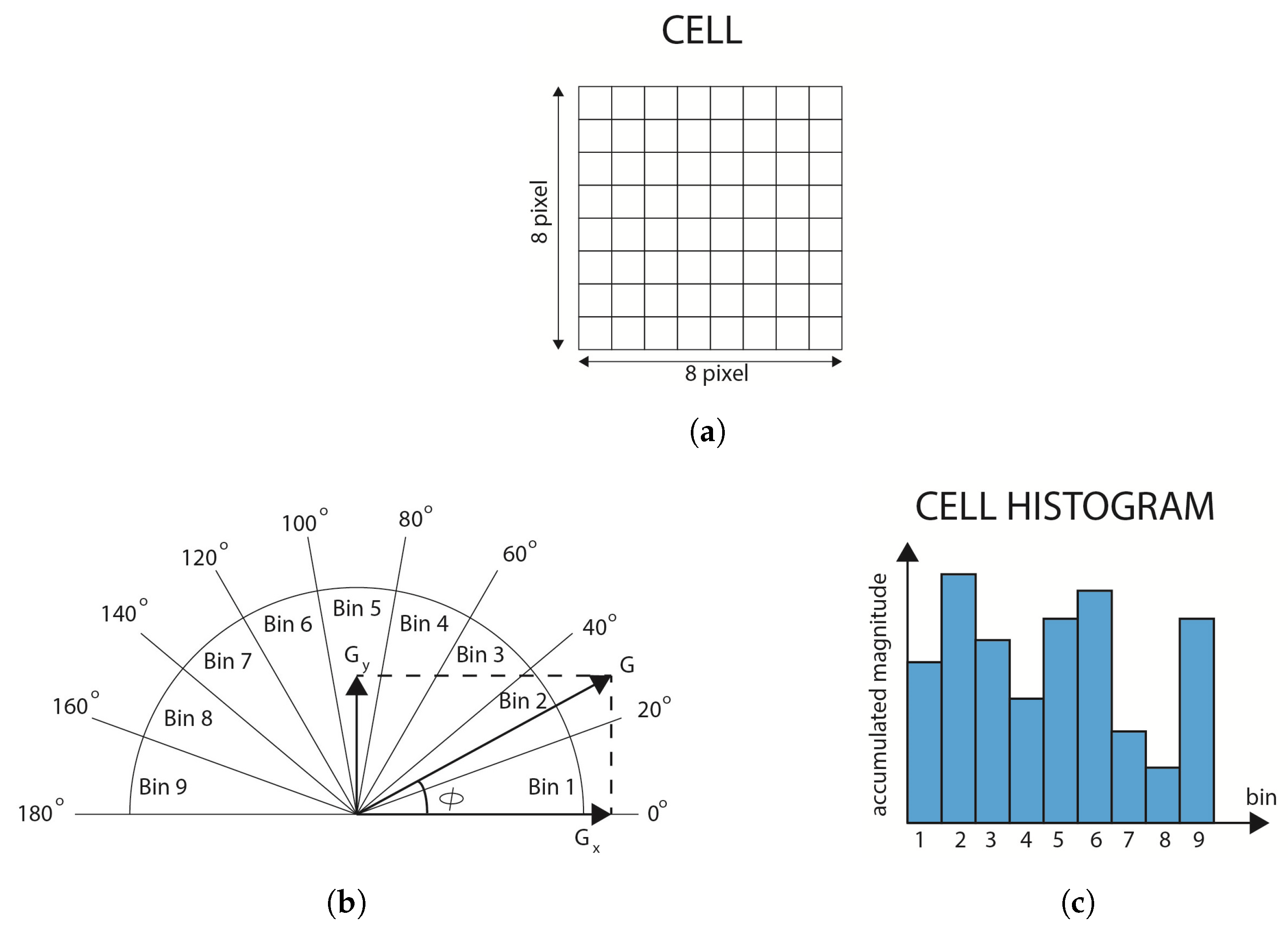
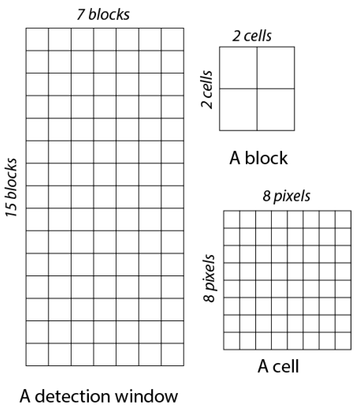
3. HOG Overview

The HOG algorithm consists of two main steps: gradient computation and histogram generation. To compute the gradient of a $pixel(x,y)$, first, we need to calculate the intensity difference of its two pairs of neighbor pixels in horizontal and vertical directions following Equations (1) and (2) respectively.

$$G_x(x,y)=I(x+1,y)-I(x-1,y)$$

(1)

$$G_y(x,y)=I(x,y+1)-I(x,y-1)$$

(2)

Then, the magnitude and the orientation of the gradient at pixel $(x,y)$ are computed by Equations (3) and (4).

$$\mid G(x,y)\mid =\sqrt{G_x{(x,y)}^2+G_y{(x,y)}^2}$$

(3)

$$\varphi (x,y)=arctan\frac{G_y(x,y)}{G_x(x,y)}$$

(4)

The histogram is generated cell by cell with those gradients. Figure 1 describes an example in detail. HOG feature is calculated cell-wise. Each cell has a size of $8\times 8$ pixels. Therefore, a cell consists of 64 pairs of magnitude and orientation gradient values. Depending on its associated orientations, magnitude gradients are accumulated to the corresponding bins. A cell histogram with nine bins is illustrated in Figure 1c. Figure 1b describes in detail how the orientation of the gradient is quantized into a range of 9 bins using the scale from 0 to 180°. The magnitude G, in this example, should be accumulated to bin 2 because its orientation is approximately 30°. For more accuracy, G could be accumulated fairly between adjacent bins depending on its orientation.

Figure 1. An illustration of how HOG features are generated. (a) Feature is calculated based on a cell of $8x8$ pixel; (b) Each pixel has a magnitude gradient G, and orientation gradient $\varphi$ ranged from 0 to 180°; (c) Each pixel contributes its magnitude gradient to the appropriate bin among 9 bins to generate the final HOG feature vector of a cell.

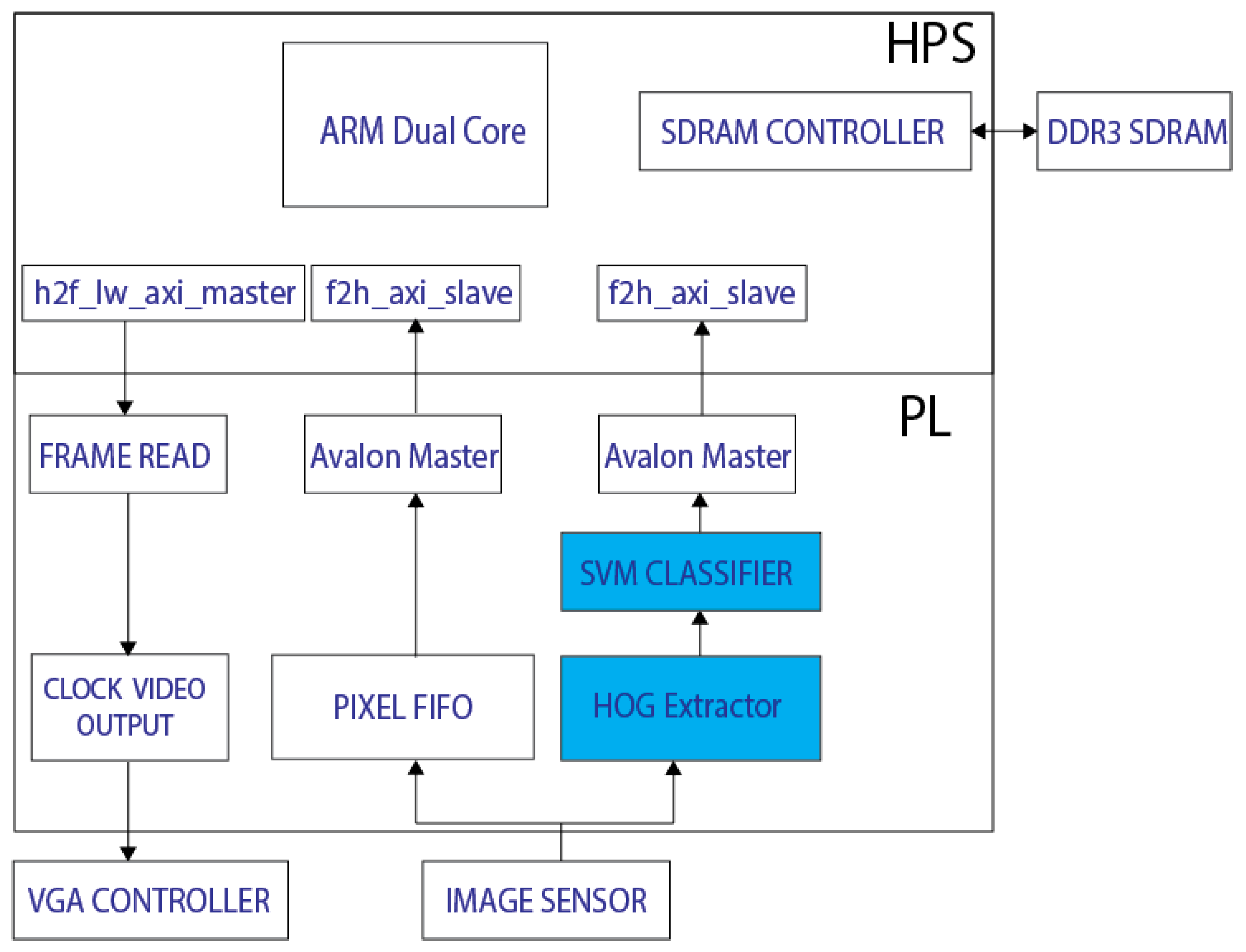
4. Implementation

We implement the whole system in Terasic’s DE1-SOC board. The system block diagram is shown in Figure 2. It includes hardware components such as the image sensor, the HOG pipeline, the Hard Processor System (HPS), and other supporting modules.

Figure 2. System diagram.

Images from the sensor, after being filtered by the Bayern Pattern, are transferred directly to both the HOG Extractor module and the pixel FIFO. The pixel FIFO is necessary for later showing the original image on the VGA. A custom Avalon master interface is created to get pixels from this FIFO and write to the 1 GB external SDRAM controlled by the HPS. The image sensor is configured through an I2C interface for some key parameters such as image size, pixel clock. The Bayer pattern filter module takes raw input pixels and calculates the three colors pixel values. After that, the grayscale pixel value is generated to provide the HOG Extractor module and the HPS for real-time visualization. The HOG extractor module is a long pipeline that generates the normalized hog features. Our best implementation in throughput used a 155 stages pipeline.

The normalized HOG features are then read by the SVM Classifier pipeline to detect pedestrians. The classifier generates the confidence values for all the sliding windows and passes them to the HPS. The confidence values are written to the external DDR3 SDRAM memory by a custom Avalon Memory-Mapped Master via the $f2h\_axi\_slave$ bridge. Similarly, another custom Avalon bus master is used to send image pixels to the DDR3 memory. These two memory locations are set to be dedicated to FPGA. This transfer method provides good performance because data are transmitted in parallel with the HPS’s CPU execution. Finally, based on a given threshold, a Python code running on the HPS will draw a bounding box at the window position in which the confidence value is higher than the threshold.

In the opposite direction, the pixels in the memory and detection results are sent to the VGA controller for real-time visualization.

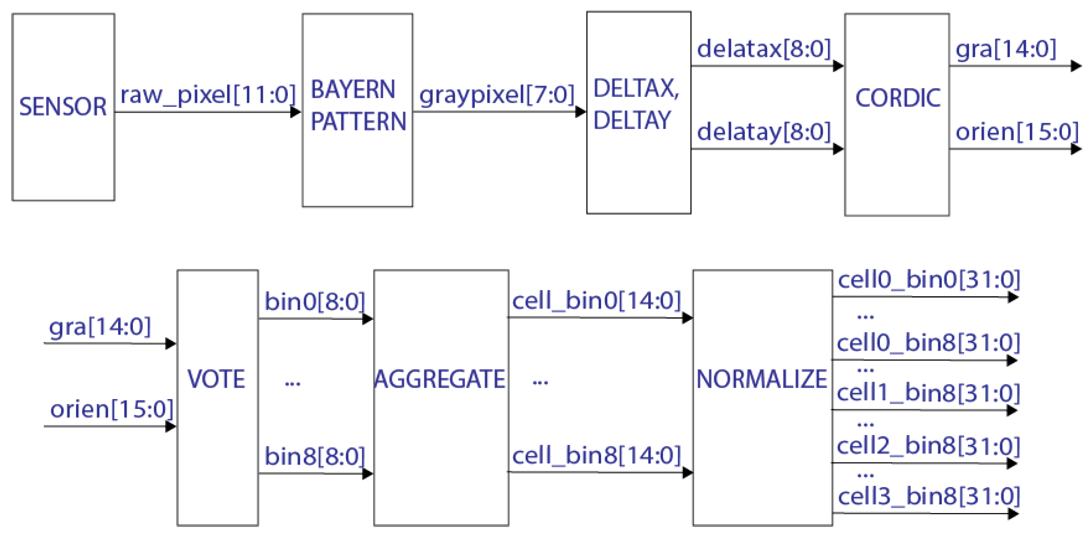
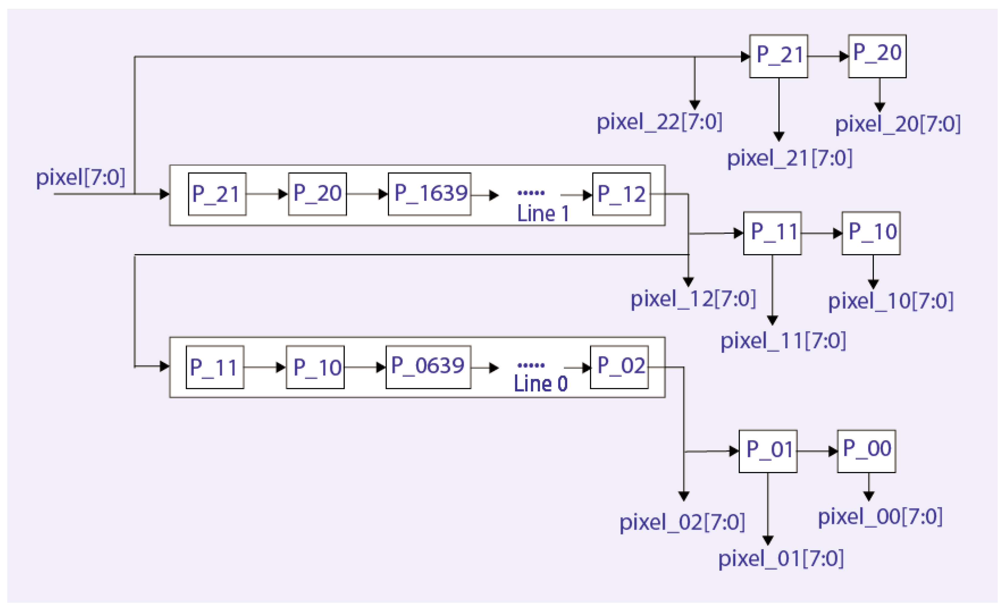
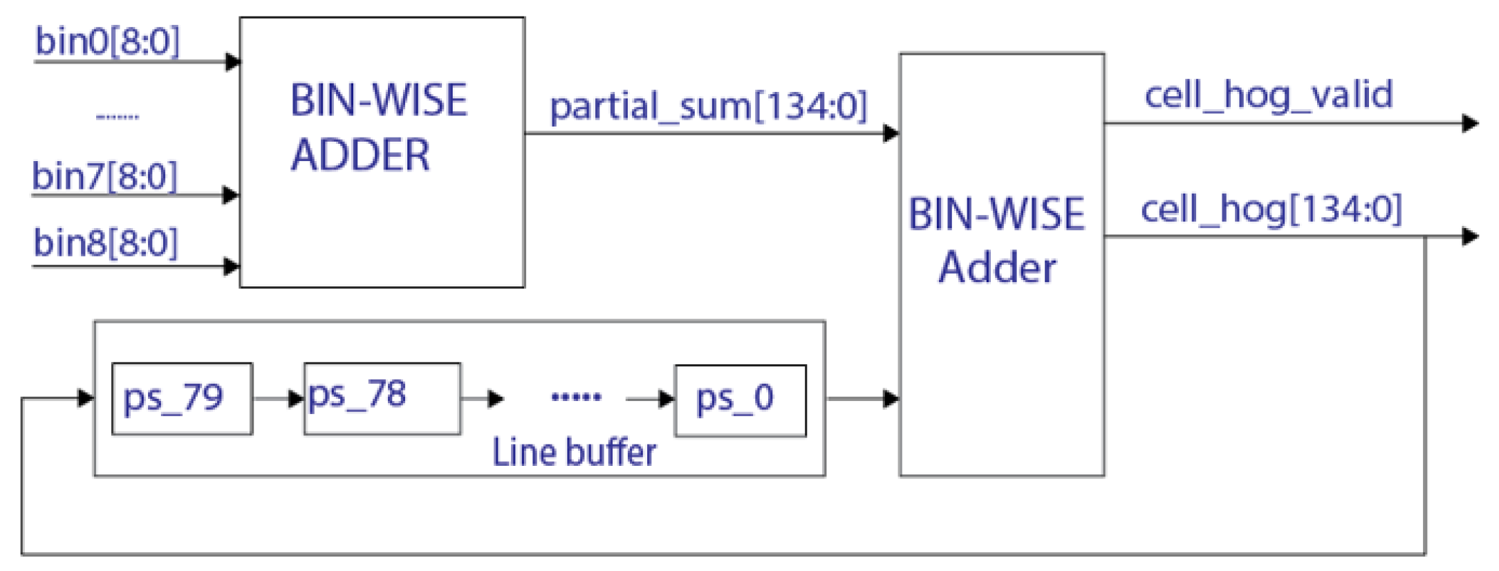
4.1. HOG Extractor

The detailed architecture inside the HOG pipeline is presented in Figure 3.

Figure 3. HOG extractor block diagram.

First, luminance differences $G_x$ and $G_y$ (Equations (1) and (2)) are calculated by the DELTAXY module. These are 9 bit signed integers. We used the vector translate function in CORDIC IP to compute the magnitude and the orientation gradients. Both of them are fixed-point numbers. To achieve two digits after the decimal point accuracy, we choose to represent the orientation gradient by 13 fractional bits. Thus, the number of fractional bits for the magnitude gradient is six, according to the configuring requirement of CORDIC IP. Depending on the orientation gradient, the magnitude gradient of each pixel will vote to appropriate bins. The AGGREGATE module adds 64 histogram values of 64 pixels in a cell bin by bin to output the final cell features. Finally, cell features are block-wise contrast normalized. In this design, each block has four cells and L2 normalization [1] is chosen for the sake of accuracy and simplicity.

Figure 4 describes our hardware line buffers that allow the HOG module to compute the luminance difference $G_x$ and $G_y$ between neighbor pixels in vertical and horizontal directions. This design supports processing pixels on every clock cycle, which means that the performance of the design can be boosted if input pixels come at every clock cycle. The depth of each buffer corresponds to the row size of the input image, in our case 640. The luminance differences, $G_x$ and $G_y$, at pixel $P_{11}$ are calculated using $P_{21}$ and $P_{01}$ for the vertical direction, and $P_{10}$ and $P_{12}$ for horizontal direction as in Equations (5) and (6).

$$G_x(1,1)=P_{10}-P_{12}$$

(5)

$$G_y(1,1)=P_{01}-P_{21}$$

(6)

Figure 4. Pixel line buffers.

Following the original HOG algorithm in [1], the final HOG feature is extracted from every cell of $8\times 8$ pixel size. In addition, the orientation is divided into 9 bins from 0 to 180°. In our case, with the $640\times 480$ image size, the final HOG feature is a vector of $80\times 60\times 9$ dimension. The HOG module processes in a pipeline approach every 8 continuous pixels in a row of a cell. It generates a partial hog vector with 9 bins aggregating 8 magnitude gradient values. These partial hog vectors are fed to a line buffer, as shown in Figure 5. Only 80 partial cell hogs are needed to be stored to minimize memory usage without stalling the pipeline. To generate the full HOG feature for a cell, it is necessary to aggregate 8 partial cell hogs from 8 different rows. The $cell\_hog\_valid$ signal will be active only if all the partial cell hogs are fully collected.

Figure 5. Partial cell hog line buffer.

The normalization of the cell histogram is done following the equation in (7). In the equation, v is the cell hog features in the block, and ${\parallel v\parallel }_2$ is the L2-normalization of all the cell hog features in the block. A small constant, $ϵ$, is added to avoid dividing by zero. As illustrated in Figure 3, each bin of the normalized hog feature is represented by 32 bits. This is not the final HOG feature value and it is represented in floating-point format. We only do the conversion from the fixed-point format to the floating-point format for the final step. Intermediate results are calculated using either integer or fixed-point number representations depending on every specific task.

$$v=\frac{v}{\sqrt{{\parallel v\parallel }_2^2+{ϵ}^2}}$$

(7)

We used the ModelSim simulator and a C golden model of the HOG to verify the HOG extractor design.

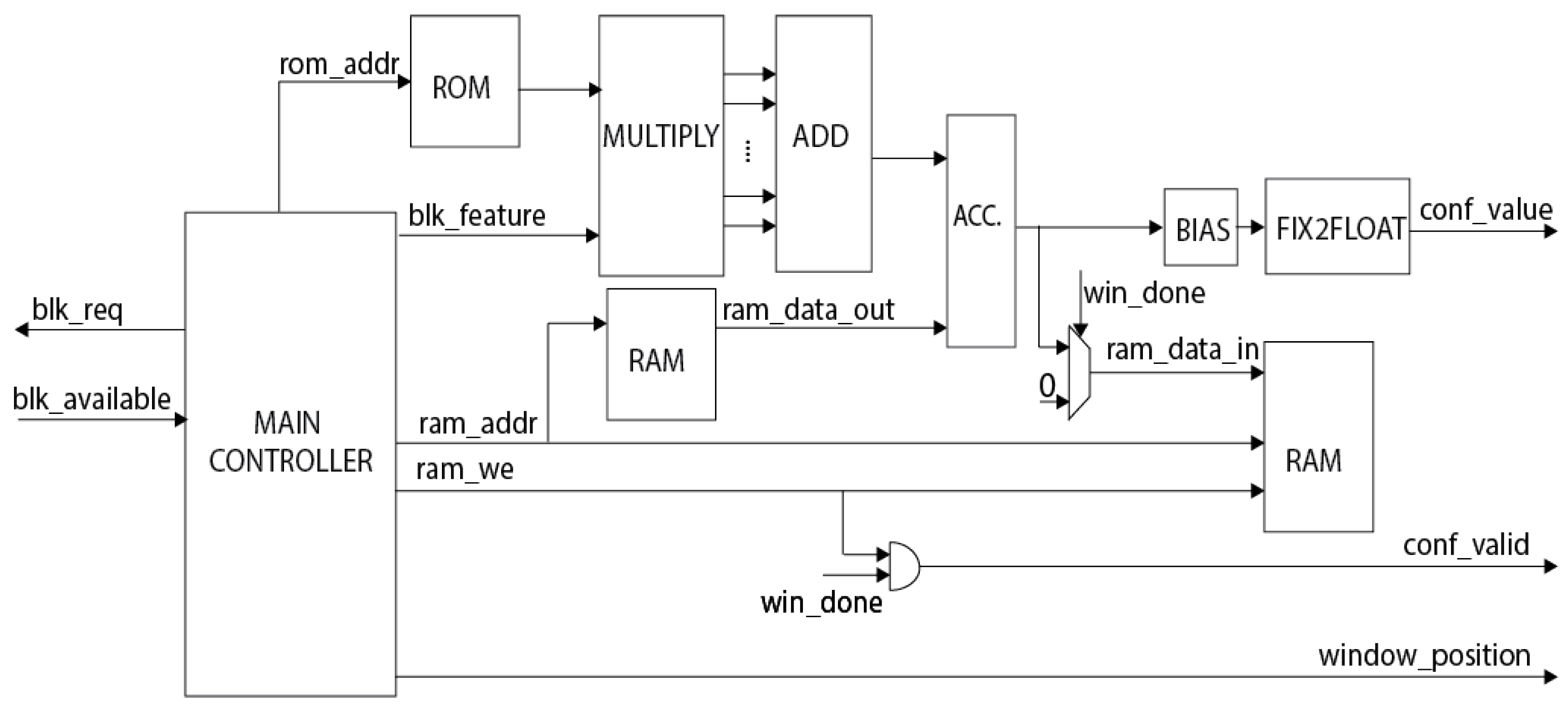
4.2. SVM Classifier

The key factor making an SVM classifier’s execution time quite long in software is the sliding window task. Figure 6 illustrates the sliding window implemented in our design. To be more specific, the size of the input image is $640\times 480$. The HOG feature of an image is organized in blocks. Each block is a concatenation of four neighboring cells, and a cell is formed by $8\times 8$ pixels as illustrated in Figure 7. To improve the detection performance, two consecutive blocks in either horizontal or vertical direction have two overlapped cells. Therefore, an image of size $640\times 480$ would have $80\times 60$ cells and $79\times 59$ blocks.

Figure 6. Sliding a 7 × 15 window over a 79 × 59 HOG frame.

Figure 7. Size of a detection window, a block, and a cell.

The SVM classifier works with block unit. In Figure 6, the HOG feature of the input image has 59 rows and each row has 79 blocks. The detection window has a size of $7\times 15$ blocks [1]. Figure 6 shows two detection windows drawn by dash lines with one block sliding step in the horizontal direction. Therefore, it takes 73 steps to slide horizontally. Similarly, in the vertical direction, there are 45 detection windows if the sliding step is one block. At each step, all 105 blocks containing 3780 fixed-point numbers in the detection window multiply with the 3780 elements of the weight vector stored in a ROM memory. Then the sum of all those 3780 products is added to the bias provided by the pre-trained model to obtain the final confidence value for that specific window. This process is repeated for $73\times 45$ detection windows. The detail accelerator of the classifier is presented in Figure 8. From the hardware point of view, there are two main problems to tackle to speed up the execution time compared to software implementation. Firstly, since blocks are generated sequentially, it is more efficient to process every block immediately after its being generated instead of waiting for the whole 105 blocks.

Figure 8. SVM classifier hardware block diagram.

In Figure 8, although the hardware design is pipelined for high throughput, the pipeline registers are not shown for the sake of clarity. Each hardware component will be briefly described in the following paragraphs.

• MAIN CONTROLLER: Finite state machine (FSM) that controls the whole design. Once a block is processed, it will check if a new block is available before fetching it to the pipeline. Knowing the block position, the FSM can infer at what detection windows belong that block. Besides, the FSM generates appropriate addresses to access ROM and RAM memory.
• ROM: this memory stores all the elements of the weight vector. If the pre-trained model is changed, that ROM must be reloaded with the new weight vector set. The size of this ROM is $3780\times 10$ bits. It means that each element of the weight vector is represented by a 10-bit fixed-point, in which 8 bits are fractional bits. To generate the weight vector, we trained and tested several models with different configurations using the INRIA Person Dataset [1] to achieve maximum yield in terms of accuracy. We tested our model with INRIA test dataset and with images coming from a camera sensor to have a more generalized model.
• RAM: there are two RAM instances in Figure 8 to distinguish between the reading and the writing process. Physically, there is one unique RAM module in the design. The memory, which has a size of $30\times 73\times 19$ bits, stores temporary sums for final confidence values. Each word is 19-bit width including a 12-bit partial sum and a 7-bit counter. Each resulting confidence value of a detection window is a sum of 105 partial sums. Therefore, the counter is used to signify that the detection window’s confidence value is valid. The $win\_done$ signal is active when 105 partial sums of a detection window are fully accumulated. Furthermore, to optimize the on-chip memory usage, the memory location storing that window’s value will be reused for other detection windows. Therefore, the design uses only $30\times 73$ RAM locations to store the temporary sums of the $45\times 73$ detection windows.
• MULTIPLY: this module takes a hog block and multiplies it with appropriate elements of the weight vector stored in the ROM memory. One-cycle multiplication will generate 36 products because a block contains 36 elements. Depends on the position of the block, it might belong to multiple detection windows. It would take 105 cycles to finish processing a specific block if that block belongs to 105 detection windows.
• ADD: This module simply sums up 36 products from the MULTIPLY module.
• ACC.: Since a detection window’s confidence value is the sum of 105 partial values. This module accumulates the temporary value stored in the RAM memory with the new partial sum.
• BIAS: This module adds the bias value to generate the final confidence value in fixed-point representation.
• FIX2FLOAT: Fixed-point confidence values are converted to 32-bit floating-point numbers by this block. From the right side of Figure 8, we can see that each confidence value is accompanied by a valid signal and an address indicating the position of that detection window in the image. This coordination is used by the HPS software to draw the rectangular if the confidence value is higher than the threshold or, in other words, a pedestrian is detected.

4.3. Number Representation

In this work, we used fixed-point numbers for all the calculations to achieve high accuracy in the detection system. The inputs to the MULTIPLY block are two fixed-point numbers, both have eight fractional bits. Although the MULTIPLY generates 16-bit fractional fixed-point numbers, only eight fractional bits are kept and feed the ADD module. This is reasonable since the 16-bit fractional number representation increases the system resources without adding accuracy. At the end of the pipeline, final confidence values are converted from fixed-point to floating-point instead of doing it by the HPS software. Owing to the use of fixed-point numbers, final scores, ranging from 0 to 1, have a 2 decimal place accuracy compared to the floating-point-based C golden model.

5. Results

To validate the design, each block is functionally validated against a reference C golden model. The golden model is implemented using floating-point arithmetic. Our hardware blocks are implemented using fixed-point arithmetic. Each block was adapted so that the maximum total error rate with respect to the golden model is 1%, which we validated to have no impact on the detection rate of the whole system.

Table 1 compares our implementation to the state-of-the-art. Regarding FPGA resources, our design is optimized for memory (what also affects energy) and therefore consumes the least memory resource except for the one in [9] which reports zero memory usage. The reason for this is that our pipeline works on every input pixel and there is not any buffer for input frames. Regarding the number of LUTs, the implementation in [7] is the most efficient, followed by ours. The reason is that, [7] targets low resource use by simplifying some computational operations. In the voting part, magnitudes are voted to only one unique bin without interpolation. To ensure the accuracy, our implementation used linear interpolation to split a magnitude into two bins unless the orientation is at the exact centre of a bin. Furthermore, all the calculations use integer numbers in [7]. About DSPs usage, our design is the second optimized. The best one only uses four DSP blocks [9]. Concerning the number of flip-flops, our design uses quite a large number of FFs to fulfill the long pipeline.

Table 1. Comparison with the state-of-the-art

Implementation	[10]	[7]	[2]	[9]	[8]	[12]	Ours
Year	2013	2013	2015	2015	2015	2018	2019
Hardware	Virtex 6	Virtex 5	Virtex 6	XC7Z020	Virtex 7	Cyclone IV	Cyclone V
Technology node	40 nm	65 nm	40 nm	28 nm	28 nm	60 nm	28 nm
Freq. (MHz)	NA	266	150	82.2	266	150	50
Frame size	1024 × 768	1920 × 1080	640 × 480	1920 × 1080	1920 × 1080	800 × 600	640 × 480
Latency	4.88 ms	<150 $\mathsf{\mu }$s	44 ms	25.2 ms	NA	NA	13.3 ms
Power (W)	182	NA	37	NA	19	NA	9
Energy (J/frame)	14	NA	0.54	NA	0.45	NA	0.12
FPS	13	64	68.2	40	42.7	162	75
Memory (Kb)	3.744	1.188	13.738	0	4.079	344	317
LUTs	108.518	5.188	184.953	21.297	30.360	16.060	13.464
DSPs	138	49	190	4	364	69	38
FFs	120.576	5.176	208.666	NA	48.576	7.220	17.117
Pixels per clock	NA	0.0005	0.0003	0.0009	0.0003	0.0009	0.0010
Energy per pixel	18	NA	1.8	NA	0.22	NA	0.39
($\mathsf{\mu }$J/pixel)
FPS per watt	0.07	NA	1.84	NA	2.25	NA	8.35

In terms of processing speed, our design takes 13.3 ms to detect a frame that correspond to a real-time throughput of 75 fps. The authors in [12] shown a throughput 2.16× better than ours with 3× faster in clock frequency. When it comes to the number of pixel processed per clock period, our design achieves the highest efficiency with 0.001 pixels per clock.

With respect to energy efficiency, we consider a resolution-independent metric such as Energy per pixel. In this case, our work is the second best after [8]. There is a difference in the measurement method. The authors in [8] used Xilinx Xpower Analyzer software to estimate the power consumption while we obtain the result from an energy meter model FHT-999. Besides, as stated in [13] some of the energy efficiency drivers for FPGA designs are the number of resources, the activity rate, and especially the technology node, which determine the dynamic power consumption. Thus, implementations on more recent 28 nm nodes benefit from this factor. For a fair comparison, the designs should be re-evaluated after mapping it to newer devices.

6. Conclusions

A low-power pedestrian detection system is implemented on a low-cost FPGA device. The power consumption of the whole system is reported to be the lowest in the state-of-the-art. Fixed-point representation is employed for achieving high accuracy with optimized resource usage. Despite that, our design achieves the highest performance in the number of pixels processed per clock. Finally, the system fulfills the real-time constraint of a pedestrian detection system with a throughput of 75 fps.

References

- Dalal, N.; Triggs, W. Histograms of Oriented Gradients for Human Detection. In Proceedings of the 2005 IEEE Computer Society Conference on Computer Vision and Pattern Recognition CVPR05, San Diego, CA, USA, 20–25 June 2005; pp. 886–893. [Google Scholar] [CrossRef]
- Ma, X.; Najjar, W.A.; Roy-Chowdhury, A.K. Evaluation and acceleration of high-throughput fixed-point object detection on FPGAS. IEEE Trans. Circuits Syst. Video Technol. 2015, 25, 1051–1062. [Google Scholar] [CrossRef]
- Ngo, V.; Casadevall, A.; Codina, M.; Castells-Rufas, D.; Carrabina, J. A pipeline hog feature extraction for real-time pedestrian detection on FPGA. In Proceedings of the 2017 IEEE East-West Design Test Symposium (EWDTS), Novi Sad, Serbia, 29 September–2 October 2017; pp. 1–6. [Google Scholar] [CrossRef]
- Ngo, V.; Casadevall, A.; Codina, M.; Castells-Rufas, D.; Carrabina, J. A low-cost SVM classifier on FPGA for pedestrian detection. In Proceedings of the Jornadas de Computación Empotrada y Reconfigurable (JCER2018), Teruel, Spain, 10–14 September 2018. [Google Scholar]
- Bauer, S.; Brunsmann, U.; Schlotterbeck-Macht, S. FPGA Implementation of a HOG-Based Pedestrian Recognition System; MPC-Workshop: Karlsruhem, Germany, 2009. [Google Scholar]
- Kadota, R.; Sugano, H.; Hiromoto, M.; Ochi, H.; Miyamoto, R.; Nakamura, Y. Hardware architecture for HOG feature extraction. In Proceedings of the IIH-MSP 2009—2009 5th International Conference on Intelligent Information Hiding and Multimedia Signal Processing, Kyoto, Japan, 12–14 September 2009; pp. 1330–1333. [Google Scholar] [CrossRef]
- Hahnle, M.; Saxen, F.; Hisung, M.; Brunsmann, U.; Doll, K. FPGA-Based real-time pedestrian detection on high-resolution images. In Proceedings of the IEEE Computer Society Conference on Computer Vision and Pattern Recognition Workshops, Portland, OR, USA, 23–28 June 2013; pp. 629–635. [Google Scholar] [CrossRef]
- Khan, A.; Khan, M.U.K.; Bilal, M.; Kyung, C.M. Hardware architecture and optimization of sliding window based pedestrian detection on FPGA for high resolution images by varying local features. In Proceedings of the IEEE/IFIP International Conference on VLSI and System-on-Chip, VLSI-SoC, Daejeon, Korea, 5–7 October 2015; pp. 142–148. [Google Scholar] [CrossRef]
- Rettkowski, J.; Boutros, A.; Göhringer, D. Real-time pedestrian detection on a xilinx zynq using the HOG algorithm. In Proceedings of the 2015 International Conference on ReConFigurable Computing and FPGAs (ReConFig), Mexico City, Mexico, 7–9 December 2015; pp. 1–8. [Google Scholar] [CrossRef]
- Blair, C.; Robertson, N.M.; Hume, D. Characterising a Heterogeneous System for Person Detection in Video using Histograms of Oriented Gradients: Power vs. Speed vs. Accuracy. IEEE J. Emerg. Sel. Top. Circuits Syst. 2013, 3, 236–247. [Google Scholar] [CrossRef]
- Bilal, M.; Khan, A.; Karim Khan, M.U.; Kyung, C. A Low-Complexity Pedestrian Detection Framework for Smart Video Surveillance Systems. IEEE Trans. Circuits Syst. Video Technol. 2017, 27, 2260–2273. [Google Scholar] [CrossRef]
- Luo, J.H.; Lin, C.H. Pure FPGA Implementation of an HOG Based Real-Time Pedestrian Detection System. Sensors 2018, 18. [Google Scholar] [CrossRef] [PubMed]
- Castells i Rufas, D. Scalable Parallel Architectures on Reconfigurable Platforms. Ph.D. Thesis, Autonomous University of Barcelona, Bellaterra, Spain, 2016. [Google Scholar]