Stress Measurement by Spectrum Analyses for Round Bar Subjected to Time-Varying Load ^†

Abstract

In this research, a feasibility study to measure the magnitude and cycle of the time-varying stress of a specimen using the natural frequency was carried out. An experiment was conducted. We used a round bar with 8 mm diameter and 290 mm span length as a specimen, which was fixed at both ends. A sinusoidal axial stress was applied to the bar. The deflection of the bar in free vibration was measured using a laser beam displacement device. To collect more information on the deflection, a device was made, which hit the bar periodically. The fast Fourier transform method, short-time Fourier transform method and wavelet analysis were applied to the deflection. The methods gave us relations among time, frequency and magnitude of the signal, with complicated representations. Applying the analyses to the experimental data, we tried to evaluate the magnitude and cycle of a time-varying load.

1. Introduction

Members of a structure or a machine are generally subjected to dynamic and periodic loads. Being fabricated into a machine, they are expected to cooperate to suspend heavy burdens. If we could evaluate with ease the magnitude and cycle of a time-varying load, it would offer us a fair evaluation of their integrity.

Strain gauges have been used to measure the stress of structures and machines. The method is simple and reliable. New kinds of strain gauges, like semiconductors and piezoelectric elements, have been developed. A Fiber Bragg Grating sensor was employed for health monitoring of a structure or a composite material [1]. In order to apply the method to a structure or a machine, we need many gauges. Measurement by strain gauges takes a lot of labor and is accompanied by troublesome work, and is unsuitable to measure working stress over a long period.

Other kinds of methods to estimate strain distribution over an area have been developed. These include the digital image correlation method [2] or the acoustic-elastic method [3]. These methods need to compare a picture or a property before and after the deformation of a structure or specimen. The procedure is still complicated and is not easily employed on site.

We applied a fast Fourier transform (FFT) method to a sound brought about by an impact with a round bar under a stationary axial load. We investigated a relation between the natural frequency and the axial stress of the bar with fix-supported ends and with simply-supported ends. The theoretical relations and experimental results were in agreement. This agreement enables us to measure the axial stress of a bar under these ends using the natural frequency [4].

In this research, we tried to evaluate the magnitude and cycle of a non-stationary load submitted to a bar specimen by a natural frequency. An experiment was conducted. We applied a sinusoidal load to the bar and measured the deflection of the bar in free vibration. Time-frequency analyses were applied to the deflection variation.

2. Theories and Experiments

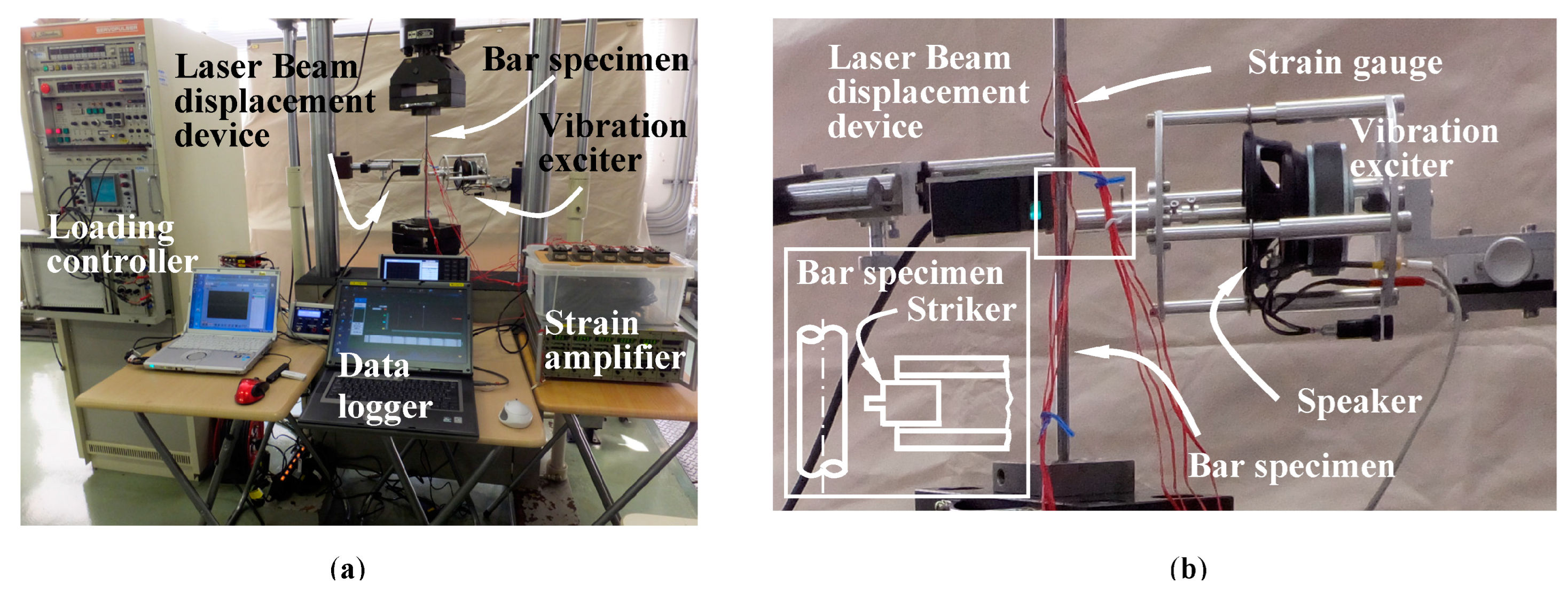
2.1. Experiment System

A round bar specimen with 8 mm diameter, 290 mm span length and fix-supported ends was used in the experiment. We measured the deflection of the bar in free vibration to evaluate the natural frequency. However, the deflection dies away in an instant. To collect more information on the deflection, we made an exciter to deliver impacts to the bar periodically. We measured the deflection of the bar using a laser beam displacement device and axial stress by strain gauges attached to the bar. The loading and measurement systems are shown in Figure 1.

We evaluate the axial stress of the bar using natural frequency. In the evaluation, we need material properties such as elastic modulus and density. The material was a rolled carbon steel for cold-finished steel bars. We obtained its density as 7.84 g/cm³. We measured its elastic modulus employing the relation given by Formula (1) between the elastic modulus and the natural frequency of the specimen suspended in the air. For the measurement, we used a specimen with 8 mm diameter and 100 mm length cut out from the same lot as the bar specimen. The elastic modulus was 210 GPa.

$$f_{p-\mathrm{th}}=\frac{1}{2\pi L^2}\sqrt{\frac{EI}{\rho A}}{({\lambda }_{p-\mathrm{th}}L)}^2$$

(1)

here, f_p-th is the natural frequency, L is the specimen length, A is the area, ρ is the density, E is the elastic modulus, I is the second moment of area and (λ_p-th L) is the eigen value.

2.2. Time-Frequency Analyses

We employed an FFT method, a short-time Fourier transform (STFT) method and a wavelet analysis. These methods and their analysis are now employed in various fields and are explained in detail elsewhere [5,6]. We leave out their explanations. An FFT gives us clear information on frequency, but does not provide any information on time. For a non-stationary load, a frequency-domain representation changes over time. The STFT method and wavelet analysis are expected to give us the relation among time, the natural frequency, and the magnitude of the signal.

2.3. Simulation Model

The angular natural frequency of the p-th natural mode of the bar in free vibration, ω_p-th, is a function of the applied load, σ_Load. The relation is expressed as Function (2). If you bring to mind tuning a guitar, this situation can be understood. If you pull a string and give it a higher tension, the string will sound with a higher tone.

$${\omega }_{p-\mathrm{th}}={\omega }_{p-\mathrm{t}h}({\sigma }_{\mathrm{Load}})$$

(2)

We applied a sinusoidal load to the bar, as described by Expression (3).

$${\sigma }_{\mathrm{Load}}(t,{\sigma }_{\mathrm{Mean}},{\sigma }_{\mathrm{Amp}},f_{\mathrm{Load}})={\sigma }_{\mathrm{Mean}}+{\sigma }_{\mathrm{Amp}}\cdot \sin (2\pi f_{\mathrm{Load}}t)$$

(3)

here, σ_Mean is the average stress, σ_Amp is the amplitude of the stress and f_Load is the cycle.

In an analysis, we usually postulate the deflection of the p-th mode natural vibration of the bar, u_p-th (x,t), as in the next expression

$$u_{p-\mathrm{th}}(x,t)=X_{p-\mathrm{th}}(x)\cdot \exp (j{\omega }_{p-\mathrm{th}}t)$$

(4)

here, X_p-th is the p-th natural mode shape and j is an imaginary unit.

The deflection of the free vibration decays. We usually refer to the effect using the next expression.

$$u_{p-\mathrm{th}}^{\mathrm{damp}}(x,t)=u{}_{p-\mathrm{th}}(x,t)\cdot \exp (-\kappa \cdot t)$$

(5)

here, κ is the damping coefficient.

The deflection of the bar in free vibration is composed of many natural mode deflections. We express it as Expression (6).

$$u=u(t,{\sigma }_{\mathrm{Mean}},{\sigma }_{\mathrm{Amp}},f_{\mathrm{Load}})={\displaystyle \sum _{x-\mathrm{th}=1}^{\infty }{u}_{x-\mathrm{th}}^{\mathrm{damp}}(x,t)\cdot {\chi }_{x-\mathrm{th}}}$$

(6)

here, χ_p-th is the ratio of the contribution of each mode to the whole deflection. We measured this deflection.

Other variables, such as a bar length and sectional area were also included in Expression (6), but they did not vary in our experiment. They were excluded in the expression as variables. In this research, we evaluate σ_Mean, σ_Amp and f_Load using signal analysis of the 1st mode of natural vibration. We employed FlexPro [7] for the data analysis of signals.

3. Results

We measured the deflection of the bar at the middle position and the stresses at the location 20 mm up from the middle using strain gauges. We compared the stress with that obtained by spectrum analysis.

Hereafter, four kinds of figures are presented. These include one for time-stress variation, the vertical axis of which is the stress of the bar measured using a strain gauge; one for time-deflection, the vertical axis of which is the deflection of the bar measured by a laser beam displacement device; and one for the frequency-spectrum using the FFT method, the horizontal axis of which is the frequency and the vertical axis is the normalized amplitude spectrum. That for time-frequency variation using the STFT method uses the vertical axis as frequency and the shade of color in the figure shows the intensity of the normalized amplitude spectrum, which is scaled by the indicator at the right-hand side of the figure.

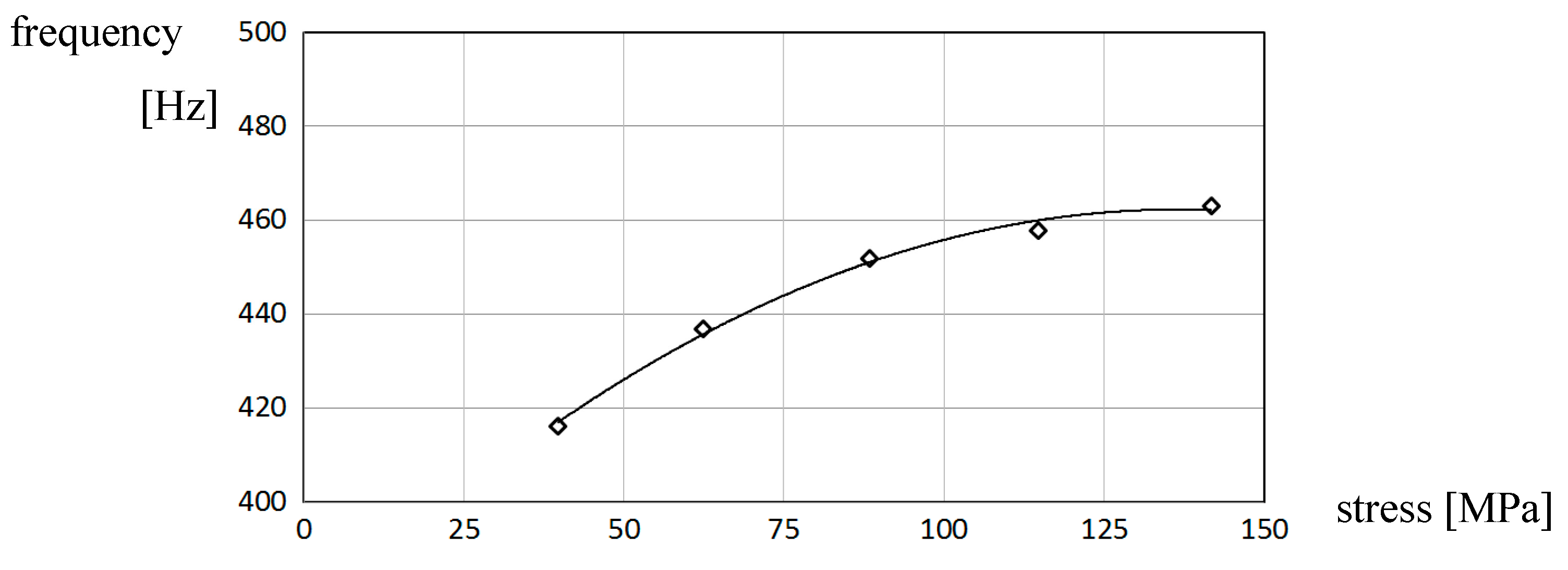
3.1. Experimental Relation between Natural Frequency and Stationary Axial Stress

Based on the experiment, we obtained the relation between the natural frequency of the 1st mode natural vibration and the stationary axial stress. The result is shown in Figure 2, which corresponds to Expression (2). Employing this relation, we can evaluate the axial stress using the natural frequency of the bar.

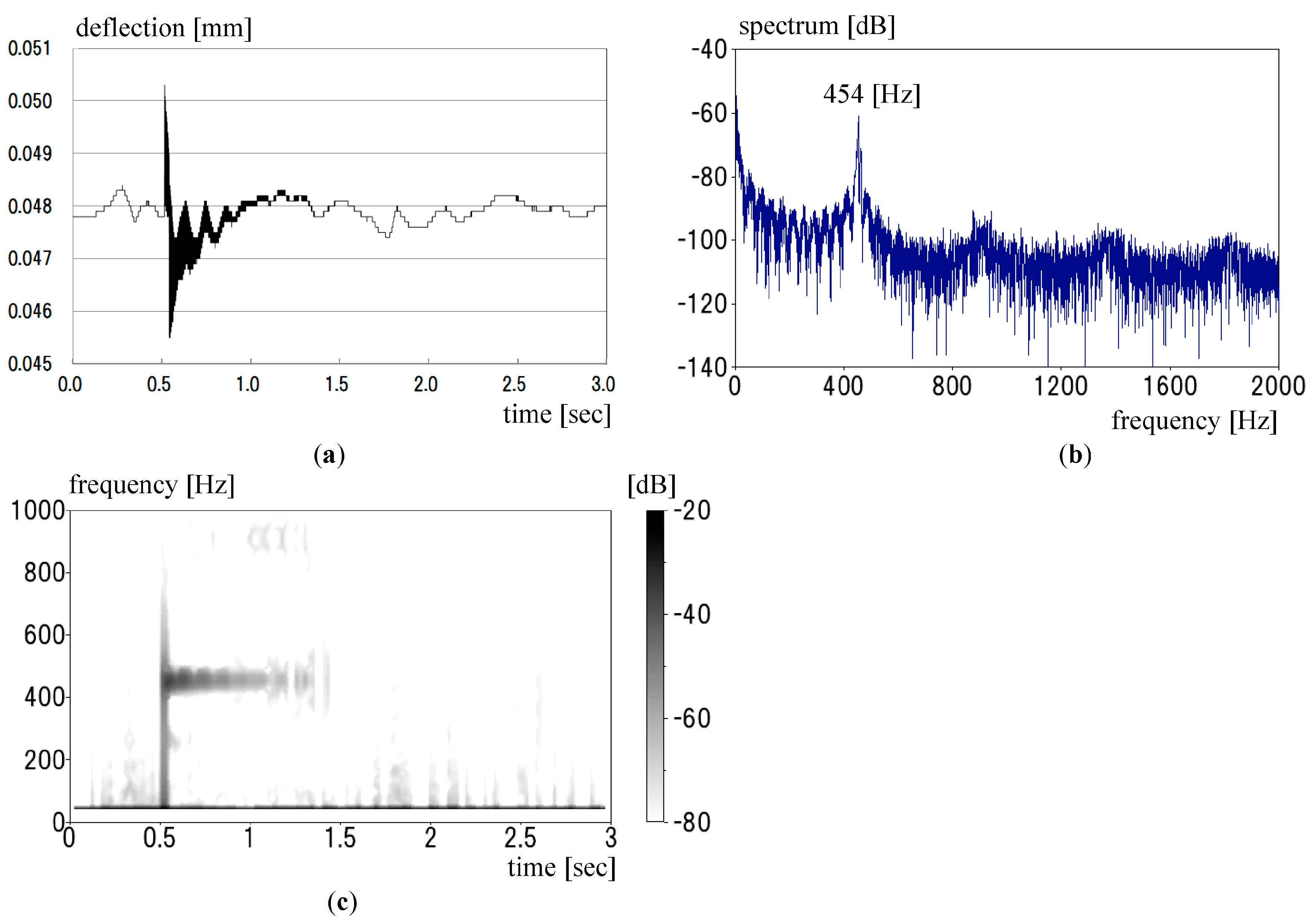
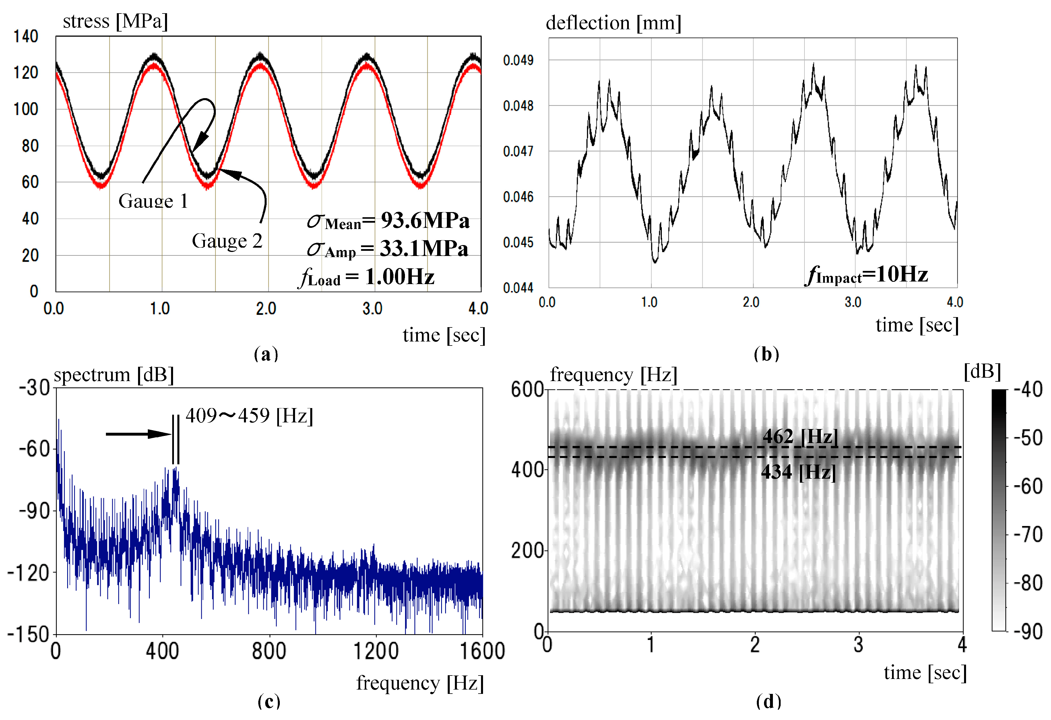
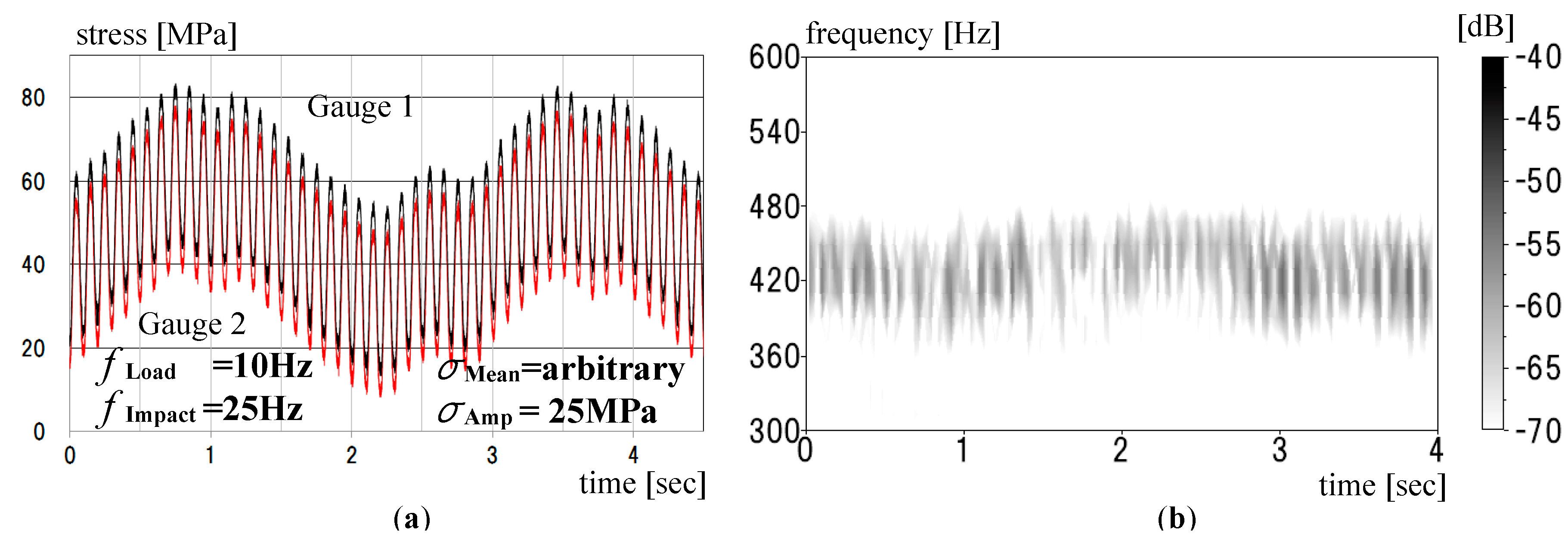
3.2. Relation between Time, Deflection and Non-Stationary Axial Stress by Experiment and Analysis

After applying a stationary load of 101 MPa to the bar, we hit the bar once to bring about a free vibration. Figure 3a shows the deflection variation of the bar. We see that the bar was impacted at around 0.5 sec and that the deflection decayed in a second.

Figure 3b shows the FFT result. We see the distinguished frequency of 454 Hz in the figure. When we evaluated the stress using this natural frequency through the relation in Figure 2, the stress was found to be 94.9 MPa. The stress value corresponds to that mentioned above.

Figure 3c shows the result using a STFT method. We used the Blackman window. The frequency distribution is a blur in the figure and faded out. The uncertainty principal between time and the natural frequency in a signal analysis is given by the equation ∆t·∆f > 1/(4π). We are able to obtain definite frequency by FFT analysis, but are not able to designate the time at which the frequency occurred. In a time-frequency analysis, we seek information both on time and frequency. As an outcome of the compromise because of this principle, we are forced to obtain an indistinct picture like the one in Figure 3c. However, we see that the frequency around 450 Hz occurred at around 0.5 s, continued for a second, and that then the vibration ended.

We applied a sinusoidal load, as defined by Expression (3), to the bar. Figure 4a shows the relation between time and the axial stress of the bar, as measured by two strain gauges. In the figure, we see sinusoidal stress variations. The gauges were attached to the bar just opposite. We see a slight difference between them. A small bending stress occurred. The parameters σ_Mean, σ_Amp and f_Load in Figure 4a are the averaged values of the two stresses.

Figure 4b shows the relation between time and the deflection of the bar by the sinusoidal load and impacts. The f_Impact in Figure 4b is the exciting frequency of the impacts to bring about free vibrations to the bar using the striker, as shown in Figure 1b. In Figure 4b, we see small ripples in the main variation of the deflection. The number of ripples coincides with the exciting frequency. The times of the horizontal axes in Figure 4a,b are not synchronized. Their times are slightly off.

We analyzed the time-deflection data in Figure 4b using FFT. The result is shown in Figure 4c. We see that peaks occur densely in the frequency range from 409 to 459 Hz. The bar loaded based on Expression (3) with the parameters in Figure 4a is expected to vibrate with a frequency of between 434 and 462 Hz, based on the relation in Figure 2.

The result using the STFT method is shown in Figure 4d. We see that a strip of a frequency varies sinusoidally at approximate 1 Hz. The same is true for the axial stress. It is difficult to evaluate definitely the range of the frequency because of the uncertainty principle. We put broken lines into Figure 4d, the frequency range obtained by the relation in Figure 2 employing the parameters in Figure 4a. If we could draw a curve which followed each peak at each time in the blurred strip, the curve would show a sinusoidal variation between the broken lines.

We applied a time-varying load to the bar, the mean stress of which was made to vary arbitrarily. The loading frequency and the stress amplitude were unchanged. The time-stress variation is given in Figure 5a. Two curves in red and black show variations of the stresses measured by strain gauges. The variation of the stress shows a saw-tooth variation. Figure 5b shows the result by STFT method. The time-frequency variation is also shown by a blurred strip for this case. However, the frequency curve peaks at each time seem to reflect the stress variation. In the next step, it will be necessary to specify definite quantification of the time-frequency variation.

4. Conclusions

We applied a time-varying sinusoidal load to a round bar. We tried to evaluate the magnitude and cycle of the stress of the bar using the natural frequency. To obtain the natural frequency, we applied impacts to the bar with an exciter to bring about a free vibration and measured the deflection of the bar. We obtained a time-stress variation pattern by spectrum analyses, but could not evaluate the magnitude of the stress definitively. We expect we will be able to obtain more detailed information on time-stress variation by accumulating our knowledge and making elaborate use of time-frequency analyses.

References

1. Moreira, P.M.G.P.; da Silva, L.F.M.; Loureiro, A.L.D. Determination of the strain distribution in adhesive joints using fiber bragg grating sensors. In Proceedings of the 15th International Conference on Experimental Mechanics, Porto, Portugal, 22–27 July 2012; pp. 581–582. [Google Scholar]
2. Leplay, P.; Rethore, J.; Meille, J.; Baietto, M.C. Identification of damage and cracking behaviors based on energy dissipation mode analysis in a quasi-brittle material using digital image correlation. Int. J. Fract. 2011, 17, 35–50. [Google Scholar] [CrossRef]
3. Kudryavtsev, Y.F. Residual Stress. In Springer Handbook on Experimental Solid Mechanics; Springer: New York, NY, USA, 2008; pp. 371–387. [Google Scholar]
4. Yoshida, T.; Takahashi, Y.; Watanabe, T.; Ain, N. Evaluation of Static Stress in Round Bar by Eigen Mode Deflection. In Proceedings of the International Conference on Advanced Technology in Experimental Mechanics, Kobe, Japan, 19–21 September 2011. [Google Scholar]
5. Christopher, T.; Compo, G.P. A Practical Guide to Wavelet Analysis. Bull. Am. Meteorol. Soc. 1998, 79, 61–78. [Google Scholar]
6. Addison, P.S. The Illustrated Wavelet Transform Handbook; IOP Publishing Ltd.: Bristol, UK, 2002. [Google Scholar]
7. FlexPro7, Data Analysis & Presentation Application; Weisang Gmbh & Co. KG: St. Ingbert, Germany, 2005.
Figure 1. Experiment system: (a) Whole arrangement; (b) Detailed configuration.
Proceedings 02 00434 g001
Figure 2. Relation between natural frequency and axial stress.
Proceedings 02 00434 g002
Figure 3. Experiment and analyzed data for stationary load from one impact: (a) Time-deflection variation; (b) Result by FFT method; (c) Result by short-time Fourier transform method.
Proceedings 02 00434 g003
Figure 4. Experiment and analyzed data for sinusoidal load: (a) Time-axial stress variation; (b) Time-deflection variation; (c) Result by FFT method; (d) Result by STFT method.
Proceedings 02 00434 g004
Figure 5. Experiment and analyzed data for load with arbitrary mean stress: (a) Time-stress variation; (b) Result by STFT method.
Proceedings 02 00434 g005
Publisher’s Note: MDPI stays neutral with regard to jurisdictional claims in published maps and institutional affiliations.