Acoustic Emission Signal Associated to Fiber Break during a Single Fiber Fragmentation Test: Modeling and Experiment †


Abstract
:1. Introduction
2. Materials and Methods
2.1. Experimental Setup
2.2. Numerical Setup
3. Results and Discussion
3.1. Experimental Results
3.1.1. Localization of AE Sources
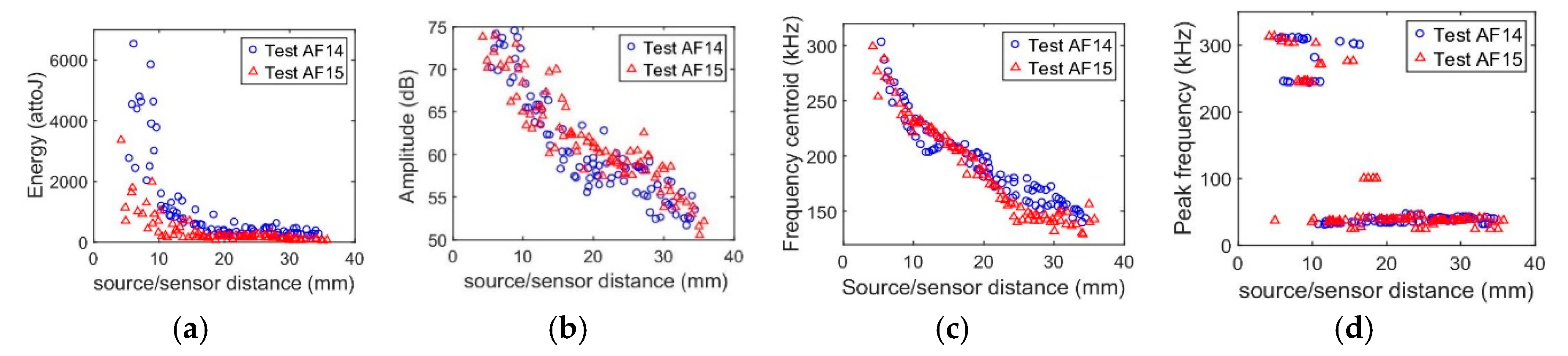
3.1.2. Effect of Distance between Source and Sensor on AE Results
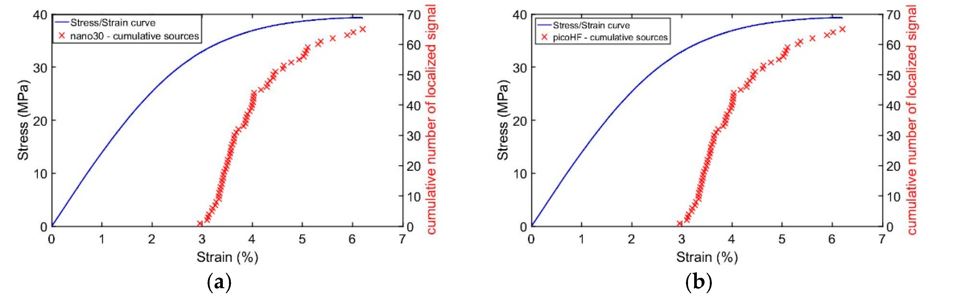
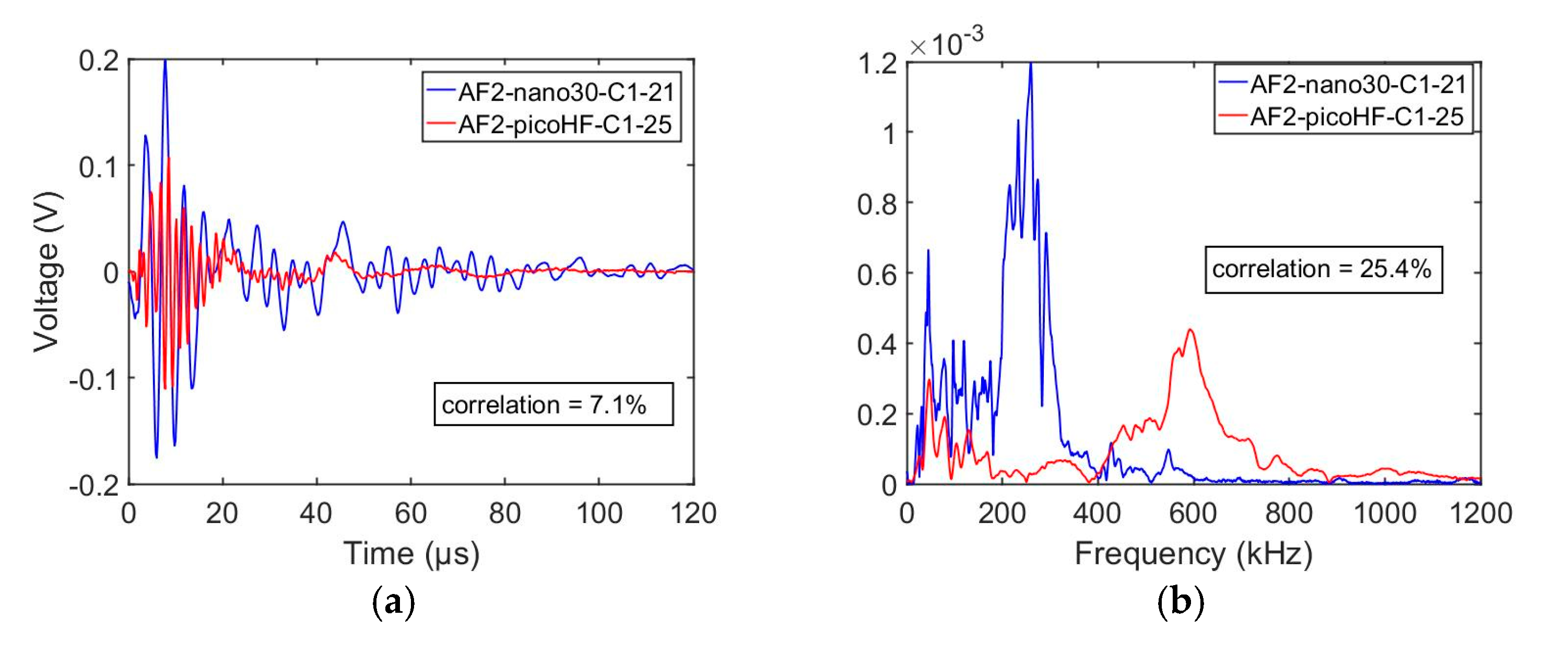
3.1.3. Effect of Sensor Type: Comparison Results of PicoHF with Results of Nano30
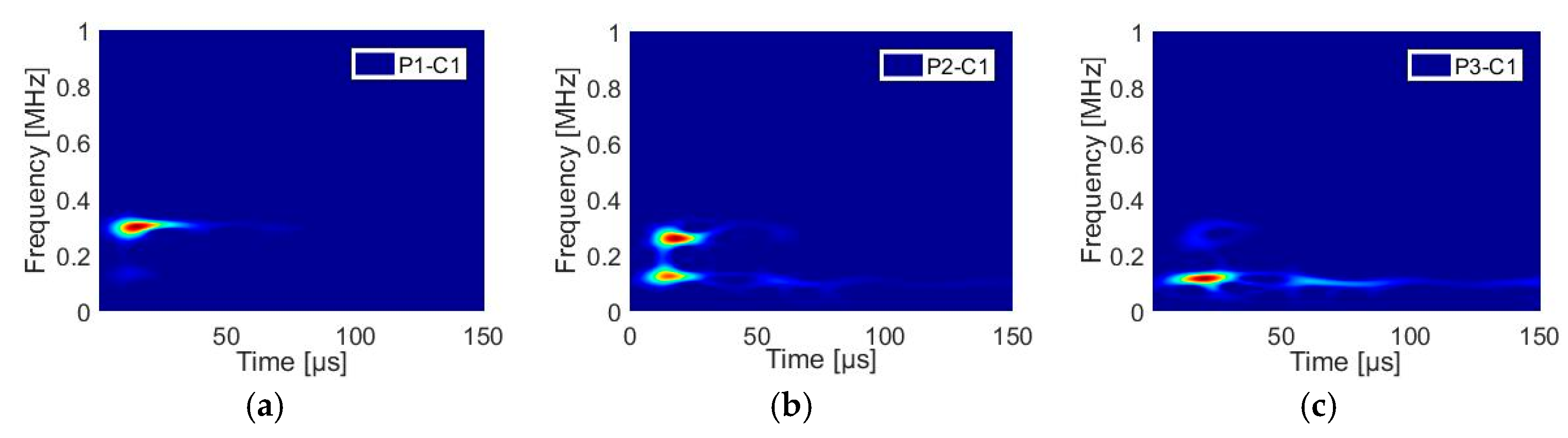
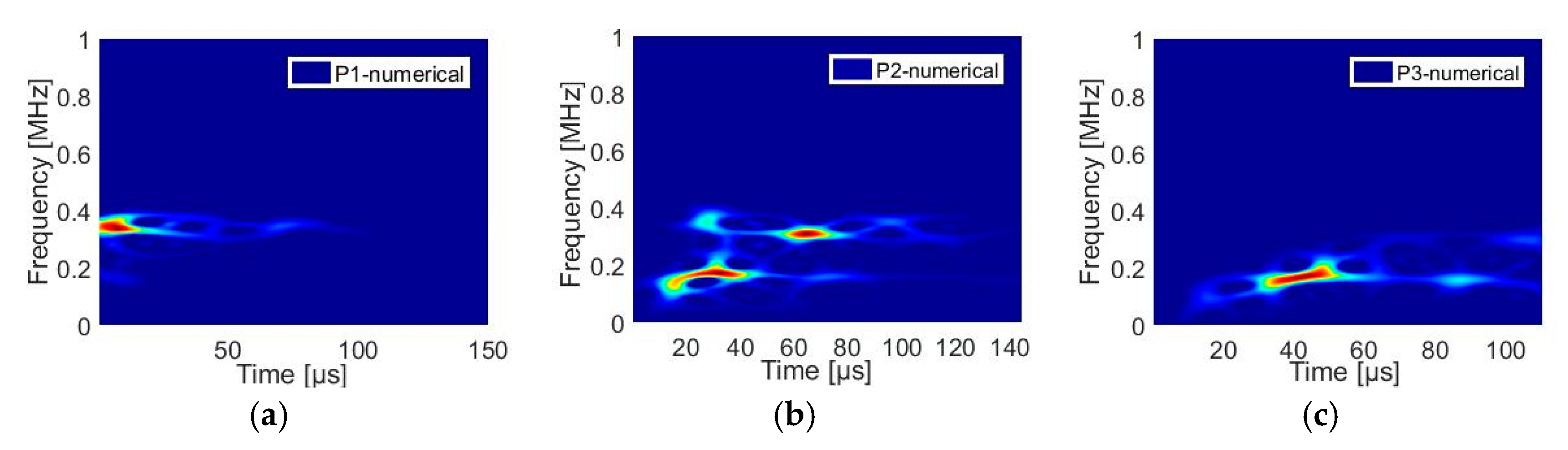
3.2. Results of the Numerical Model
3.2.1. Numerical Results without and with Sensor
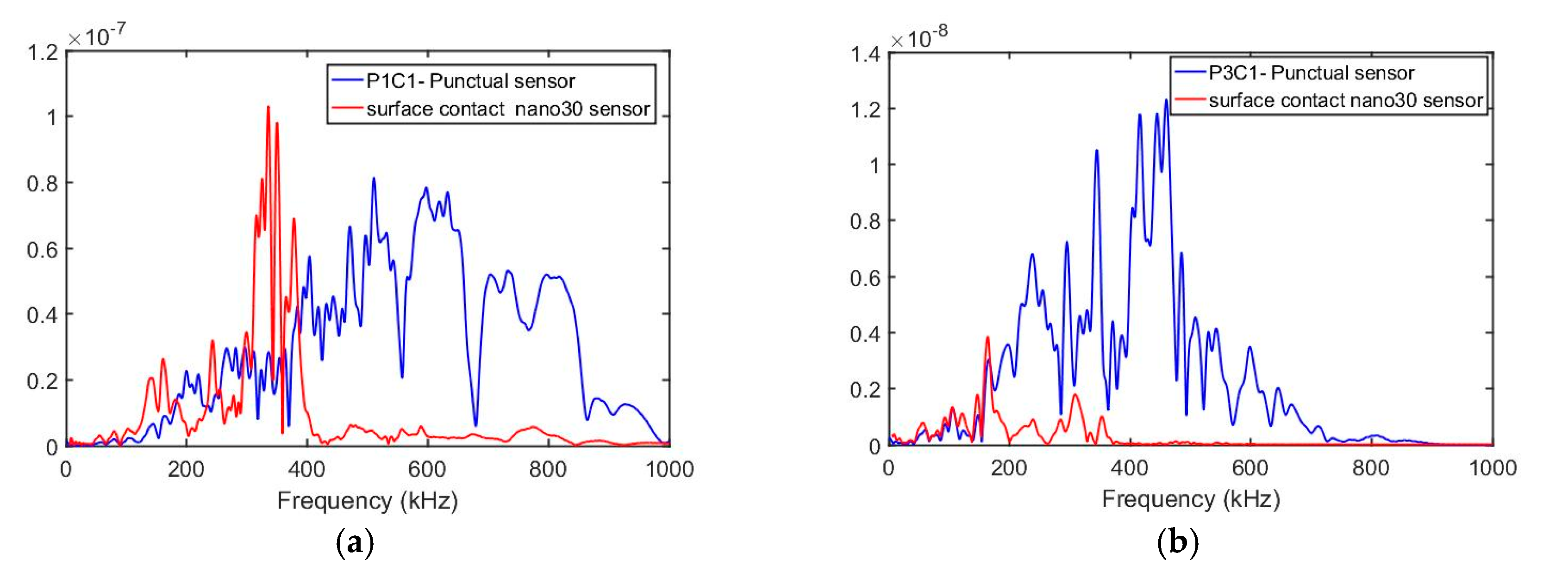
3.2.2. Comparison Numerical and Experimental Results
4. Conclusions
References
- Giordano, M.; Cndelli, L.; Nicolais, L. Acoustic Emission wave propagation in viscoelastic plate. Compos. Sci. Technol. 1999, 59, 1735–1743. [Google Scholar] [CrossRef]
- Sause, M.G.; Richler, S. Finite element modelling of cracks as acoustic emission sources. J. Nondestruct. Eval. 2015, 34, 4. [Google Scholar] [CrossRef]
- Le Gall, T.; Godin, N.; Monnier, T.; Fusco, C.; Hamam, Z. Acoustic Emission modeling from the source to the detected signal: Model validation and identification of relevant descriptors. J. Acoust. Emiss. 2017, 34, S59–S64. [Google Scholar]
- Morizet, N.; Godin, N.; Tang, J.; Maillet, E.; Fregonese, M.; Normand, B. Classification of acoustic emission signals using wavelets and Random Forests: Application to localized corrosion. Mech. Syst. Signal Process. 2016, 70, 1026–1037. [Google Scholar] [CrossRef]
- Godin, N.; Reynaud, P.; Fantozzi, G. Acoustic Emission and Durability of Composite Materials; John Wiley & Sons: Hoboken, NJ, USA, 2018. [Google Scholar]
- Monnier, T.; Seydou, D.; Godin, N.; Zhang, F. Primary calibration of acoustic emission sensors by the method of reciprocity, theoretical and experimental considerations. J. Acoust. Emiss. 2012, 30, 152–166. [Google Scholar]


| Young Modulus (GPa) | Poisson Ratio | Density (kg/m3) | |
|---|---|---|---|
| Carbon fiber | 187 | 0.22 | 1800 |
| DGEBD-3DCM | 1.41 | 0.38 | 1034 |
| Descriptors | nano30 | picoHF | ||||||
|---|---|---|---|---|---|---|---|---|
| Near to Sensor | Far from Sensor | Near to Sensor | Far from Sensor | |||||
| AF02 | AF03 | AF02 | AF03 | AF02 | AF03 | AF02 | AF03 | |
| Amplitude (dB) | 66.4 | 64 | 53.7 | 48.6 | 60.8 | 57.2 | 43.7 | 41.2 |
| Energy (attoJ) | 2332 | 320 | 260 | 15.8 | 107 | 55.1 | 8.4 | 5.2 |
| PP [0,1,2,3,4,5,6,7,8,9,10,11,12,13,14,15,16,17,18,19,20,21,22,23,24,25,26,27,28,29,30,31,32,33,34,35,36,37,38,39,40,41,42,43,44,45,46,47,48,49,50,51,52,53,54,55,56,57,58,59,60,61,62,63,64,65,66,67,68,69,70,71,72,73,74,75,76,77,78,79,80,81,82,83,84,85,86,87,88,89,90,91,92,93,94,95,96,97,98,99,100,101,102,103,104,105,106,107,108,109,110,111,112,113,114,115,116,117,118,119,120,121,122,123,124,125,126,127,128,129,130,131,132,133,134,135,136,137,138,139,140,141,142,143,144,145,146,147,148,149,150,151,152,153,154,155,156,157,158,159,160,161,162,163,164,165,166,167,168,169,170,171,172,173,174,175,176,177,178,179,180,181,182,183,184,185,186,187,188,189,190,191,192,193,194,195,196,197,198,199,200] kHz (%) | 36.2 | 35.6 | 70.5 | 72.5 | 24.5 | 25.5 | 82.5 | 78.1 |
| PP [200,201,202,203,204,205,206,207,208,209,210,211,212,213,214,215,216,217,218,219,220,221,222,223,224,225,226,227,228,229,230,231,232,233,234,235,236,237,238,239,240,241,242,243,244,245,246,247,248,249,250,251,252,253,254,255,256,257,258,259,260,261,262,263,264,265,266,267,268,269,270,271,272,273,274,275,276,277,278,279,280,281,282,283,284,285,286,287,288,289,290,291,292,293,294,295,296,297,298,299,300,301,302,303,304,305,306,307,308,309,310,311,312,313,314,315,316,317,318,319,320,321,322,323,324,325,326,327,328,329,330,331,332,333,334,335,336,337,338,339,340,341,342,343,344,345,346,347,348,349,350,351,352,353,354,355,356,357,358,359,360,361,362,363,364,365,366,367,368,369,370,371,372,373,374,375,376,377,378,379,380,381,382,383,384,385,386,387,388,389,390,391,392,393,394,395,396,397,398,399,400] kHz (%) | 53 | 55 | 25.8 | 21.8 | 10.9 | 11.4 | 7.4 | 7.5 |
| PP [400,401,402,403,404,405,406,407,408,409,410,411,412,413,414,415,416,417,418,419,420,421,422,423,424,425,426,427,428,429,430,431,432,433,434,435,436,437,438,439,440,441,442,443,444,445,446,447,448,449,450,451,452,453,454,455,456,457,458,459,460,461,462,463,464,465,466,467,468,469,470,471,472,473,474,475,476,477,478,479,480,481,482,483,484,485,486,487,488,489,490,491,492,493,494,495,496,497,498,499,500,501,502,503,504,505,506,507,508,509,510,511,512,513,514,515,516,517,518,519,520,521,522,523,524,525,526,527,528,529,530,531,532,533,534,535,536,537,538,539,540,541,542,543,544,545,546,547,548,549,550,551,552,553,554,555,556,557,558,559,560,561,562,563,564,565,566,567,568,569,570,571,572,573,574,575,576,577,578,579,580,581,582,583,584,585,586,587,588,589,590,591,592,593,594,595,596,597,598,599,600,601,602,603,604,605,606,607,608,609,610,611,612,613,614,615,616,617,618,619,620,621,622,623,624,625,626,627,628,629,630,631,632,633,634,635,636,637,638,639,640,641,642,643,644,645,646,647,648,649,650,651,652,653,654,655,656,657,658,659,660,661,662,663,664,665,666,667,668,669,670,671,672,673,674,675,676,677,678,679,680,681,682,683,684,685,686,687,688,689,690,691,692,693,694,695,696,697,698,699,700,701,702,703,704,705,706,707,708,709,710,711,712,713,714,715,716,717,718,719,720,721,722,723,724,725,726,727,728,729,730,731,732,733,734,735,736,737,738,739,740,741,742,743,744,745,746,747,748,749,750,751,752,753,754,755,756,757,758,759,760,761,762,763,764,765,766,767,768,769,770,771,772,773,774,775,776,777,778,779,780,781,782,783,784,785,786,787,788,789,790,791,792,793,794,795,796,797,798,799,800] kHz (%) | 9.4 | 7.1 | 2.2 | 3.8 | 55.3 | 36.3 | 7.2 | 8.4 |
| PP [800,801,802,803,804,805,806,807,808,809,810,811,812,813,814,815,816,817,818,819,820,821,822,823,824,825,826,827,828,829,830,831,832,833,834,835,836,837,838,839,840,841,842,843,844,845,846,847,848,849,850,851,852,853,854,855,856,857,858,859,860,861,862,863,864,865,866,867,868,869,870,871,872,873,874,875,876,877,878,879,880,881,882,883,884,885,886,887,888,889,890,891,892,893,894,895,896,897,898,899,900,901,902,903,904,905,906,907,908,909,910,911,912,913,914,915,916,917,918,919,920,921,922,923,924,925,926,927,928,929,930,931,932,933,934,935,936,937,938,939,940,941,942,943,944,945,946,947,948,949,950,951,952,953,954,955,956,957,958,959,960,961,962,963,964,965,966,967,968,969,970,971,972,973,974,975,976,977,978,979,980,981,982,983,984,985,986,987,988,989,990,991,992,993,994,995,996,997,998,999,1000,1001,1002,1003,1004,1005,1006,1007,1008,1009,1010,1011,1012,1013,1014,1015,1016,1017,1018,1019,1020,1021,1022,1023,1024,1025,1026,1027,1028,1029,1030,1031,1032,1033,1034,1035,1036,1037,1038,1039,1040,1041,1042,1043,1044,1045,1046,1047,1048,1049,1050,1051,1052,1053,1054,1055,1056,1057,1058,1059,1060,1061,1062,1063,1064,1065,1066,1067,1068,1069,1070,1071,1072,1073,1074,1075,1076,1077,1078,1079,1080,1081,1082,1083,1084,1085,1086,1087,1088,1089,1090,1091,1092,1093,1094,1095,1096,1097,1098,1099,1100,1101,1102,1103,1104,1105,1106,1107,1108,1109,1110,1111,1112,1113,1114,1115,1116,1117,1118,1119,1120,1121,1122,1123,1124,1125,1126,1127,1128,1129,1130,1131,1132,1133,1134,1135,1136,1137,1138,1139,1140,1141,1142,1143,1144,1145,1146,1147,1148,1149,1150,1151,1152,1153,1154,1155,1156,1157,1158,1159,1160,1161,1162,1163,1164,1165,1166,1167,1168,1169,1170,1171,1172,1173,1174,1175,1176,1177,1178,1179,1180,1181,1182,1183,1184,1185,1186,1187,1188,1189,1190,1191,1192,1193,1194,1195,1196,1197,1198,1199,1200] kHz (%) | 1.1 | 2.1 | 1.5 | 1.9 | 9.2 | 26.8 | 2.9 | 6 |
| Frequency Centroid (kHz) | 253 | 259 | 162 | 168 | 455 | 536 | 157 | 189 |
| Peak Frequency (kHz) | 251 | 260 | 70 | 53 | 351 | 256 | 50 | 40 |
Publisher’s Note: MDPI stays neutral with regard to jurisdictional claims in published maps and institutional affiliations. |
© 2018 by the authors. Licensee MDPI, Basel, Switzerland. This article is an open access article distributed under the terms and conditions of the Creative Commons Attribution (CC BY) license (https://creativecommons.org/licenses/by/4.0/).
Share and Cite
Hamam, Z.; Godin, N.; Fusco, C.; Monnier, T. Acoustic Emission Signal Associated to Fiber Break during a Single Fiber Fragmentation Test: Modeling and Experiment. Proceedings 2018, 2, 394. https://doi.org/10.3390/ICEM18-05222
Hamam Z, Godin N, Fusco C, Monnier T. Acoustic Emission Signal Associated to Fiber Break during a Single Fiber Fragmentation Test: Modeling and Experiment. Proceedings. 2018; 2(8):394. https://doi.org/10.3390/ICEM18-05222
Chicago/Turabian StyleHamam, Zeina, Nathalie Godin, Claudio Fusco, and Thomas Monnier. 2018. "Acoustic Emission Signal Associated to Fiber Break during a Single Fiber Fragmentation Test: Modeling and Experiment" Proceedings 2, no. 8: 394. https://doi.org/10.3390/ICEM18-05222
APA StyleHamam, Z., Godin, N., Fusco, C., & Monnier, T. (2018). Acoustic Emission Signal Associated to Fiber Break during a Single Fiber Fragmentation Test: Modeling and Experiment. Proceedings, 2(8), 394. https://doi.org/10.3390/ICEM18-05222