Impact of Water Demand Pattern on Calibration Process ^†

Abstract

Mathematical models are the basic tool that simulates the operation of the Water Distribution System (WDS). Building such a tool is a complex task that requires as much detail as possible. The information needed to build a model can be divided into two categories: network data and WDS operating data. The first group includes pipe and node attributes, such as pipe length, pipe diameter, pipe roughness, junction elevation, and junction demand. The second category includes data specifying network performance such as pump characteristics, water demand patterns, and controls. The quality of these data will reflect the quality (compatibility) of the model. In WDS modeling—especially dynamic modeling—water demand patterns will have a significant impact on model accuracy. The appearance of each pattern may be different; it depends on the type of consumption (domestic, industrial) or the period analyzed. Consumption patterns define the operational work of the WDSs. Changes in water demand patterns may affect the accuracy of the model calibration. Real WDS models were used in this paper. Three simulations were analyzed, with each corresponding to a different period: one year, six months, and one month. Junction demand and water demand patterns were generated from a GIS (Geographic Information System) and SCADA (Supervisory Control and Data Acquisition) database.

1. Introduction

Mathematical models are a basic tool used by water supply companies to support decision-making. The purpose of Water Distribution System (WDS) modeling is to reflect the operational workings of a network. The most important task is to achieve the highest possible accuracy of the WDS model, independently of the chosen period or the occurrence of failure to be analyzed. For this reason, the model is calibrated. Calibration is a process through which the physical and operational data of the WDS is determined; as a result, a coincident model of the WDS is obtained [1]. During modeling, all data that represent network graphs and WDS performance are verified. According to Walski [2], the highest uncertainty of data is related to pipe roughness and water demand. These data are verified in the final stage of calibration—micro-calibration [2,3]. Pipe roughness is dependent on the pipe diameter, material, age and water quality, which can be defined by mathematical function or systemized. Water demand is a force that determines the type of operational workings of the network.

Water demand is related to water consumption patterns and the placement of consumption points [4]. Data used to create hydraulic models are mostly based on the GIS (Geographic Information System) database, billing databases, and SCADA (Supervisory Control and Data Acquisition) systems. The location points of customers are obtained from the first database, which assigns water demand to the nearest node. While water demand (average, maximal or minimal value) and water consumption patterns are exported from the two other databases. According to the modeling algorithm, the water consumption pattern is determined by formula below [5]:

$${\mathrm{d}}_{\mathrm{i}}\left(\mathrm{k}\right){=\mathrm{d}}_{{\mathrm{base}}_{\mathrm{i}}}·\mathrm{pattern}\left(\mathrm{k}\right)$$

(1)

where:

d_i(k)—i junction water consumption at any time k

d_basei—i water consumption (value from billing databases)

pattern(k)—water consumption pattern exported from the SCADA database

The sum of momentary water consumption should equate to total daily water consumption at the node:

$${\displaystyle \sum }_{\mathrm{i}}{\mathrm{d}}_{\mathrm{i}}\left(\mathrm{k}\right)={\mathrm{d}}_{\mathrm{total}}\left(\mathrm{k}\right)$$

(2)

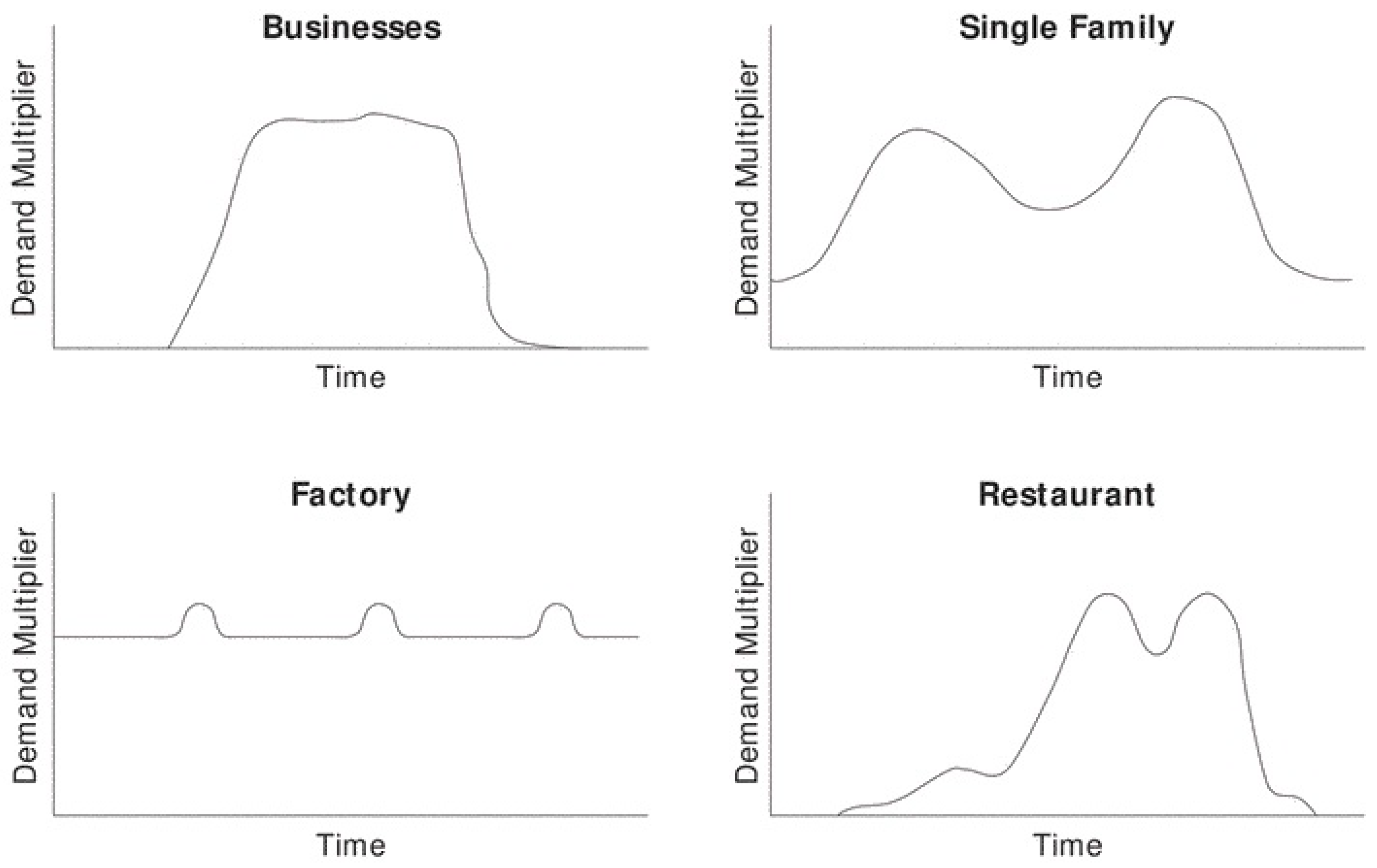
Water consumption patterns vary from each other, depending on the type of customer. There are four basic types of recipients: domestic, industry (e.g., factory), business and service (e.g., restaurant). Domestic and service areas are characterized by two maximum water demands per day, for domestic these are morning and evening, and for services there are two in the evening. Industry water consumption patterns are determined by the nature of the customers’ work—the maximum water demand may occur in the afternoon or at night—while for businesses, it is characterized by an equal water intake throughout the day (Figure 1).

Water demand also depends on seasonal changes, like spring (gardening) and summer changes. Selection of the simulation period should be preceded by precise analysis of the network operational work and water consumption, so that it reflects the normal operating work of the WDS.

2. Research Subject—Selected Area of the WDS

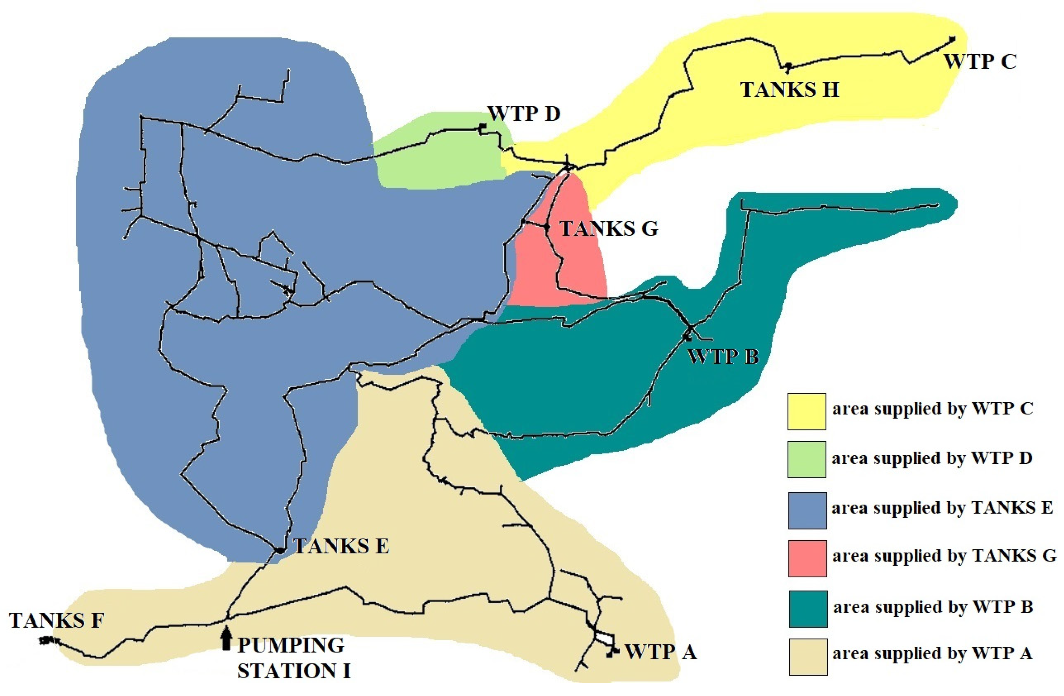
The subject of this study is the selected water supply area of the large WDS. The subsystem consists of four Water Treatment Plants (WTP A, WTP B, WTP C and WTP D) with a total daily average production of 55,000 m³ and four complexes of tanks (TANKS E, F, G and H) with a total capacity of 162,000 m³ (Figure 2). Tanks E are additionally supplied from a pumping station (PUMPING STATION I) located outside the considered area of subsystem, with an average daily amount of 60,000 m³. The average daily amount of supplied water in this area is 115,000 m³. Daily water demand for this area is 102,000 m³. The WDS under consideration is a wide network with a total length of 256 km. The water supply infrastructure is characterized by high variability of material and diameters from 55 mm to 1600 mm. The WDS is mainly made of steel (73%) and polyethylene PE-SDR17 (10.6%), with a small share of ductile iron. The oldest pipelines comprising this distribution subsystem date back to 1929 (steel wires), and the most recentto2016 (PE-SDR17).

The central point of the subsystem is the storage tanks E, which are supplied from two directions (WTP A and PUMPING STATION I), and supply water to the largest number of customers, representing nearly 50% (Figure 2 color blue). Tanks F are the boundaries of the subsystem, and in the simulations under consideration are the water receivers (normally supplied with water from five directions). Storage tanks G supplied the smallest area, due to pipe failures that occurred in the considered period. WTP D works periodically, in situations of increased water consumption (summer time) (Figure 2).

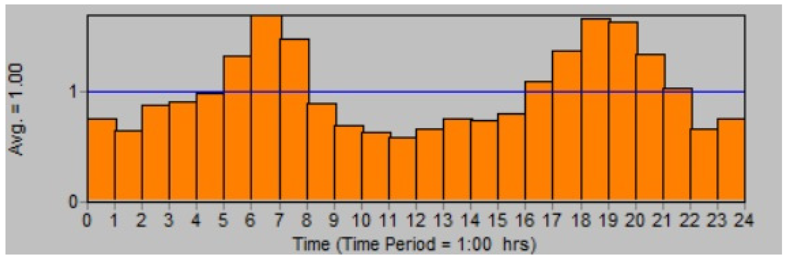
The WDS supplies an urban-industrial area with a high prevalence of urban areas (93.8%). Domestic water consumption patterns are characterized by the standard regularity of the occurrence of two peaks of water consumption in the morning and in the evening (Figure 3).

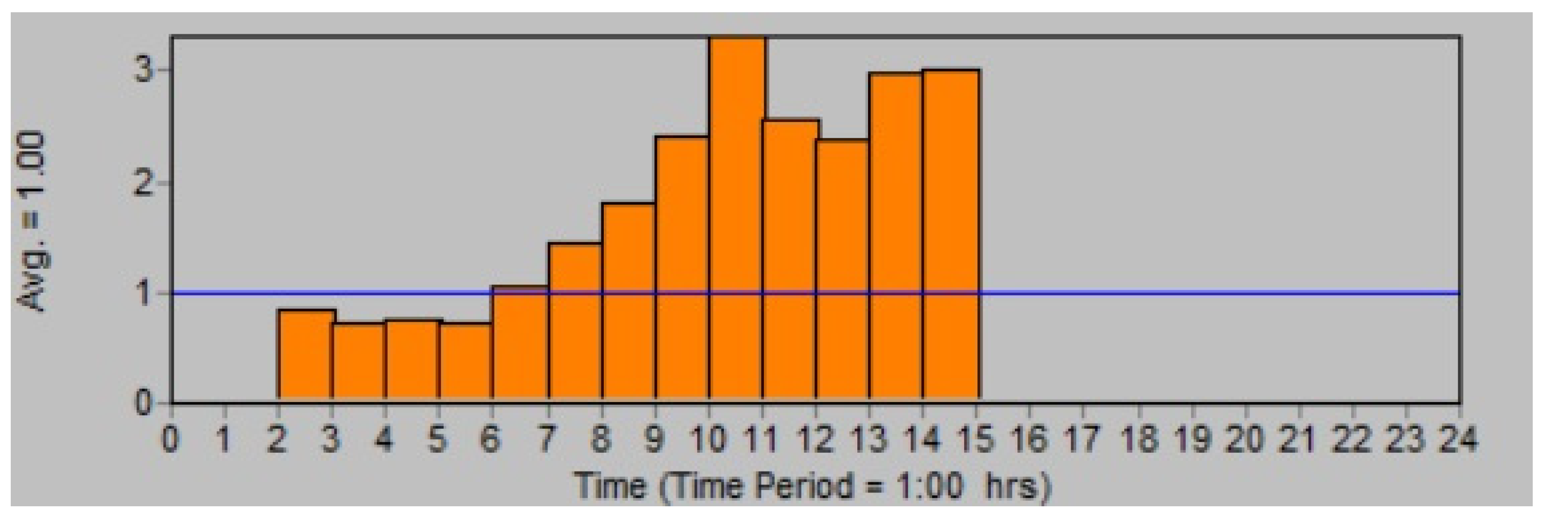
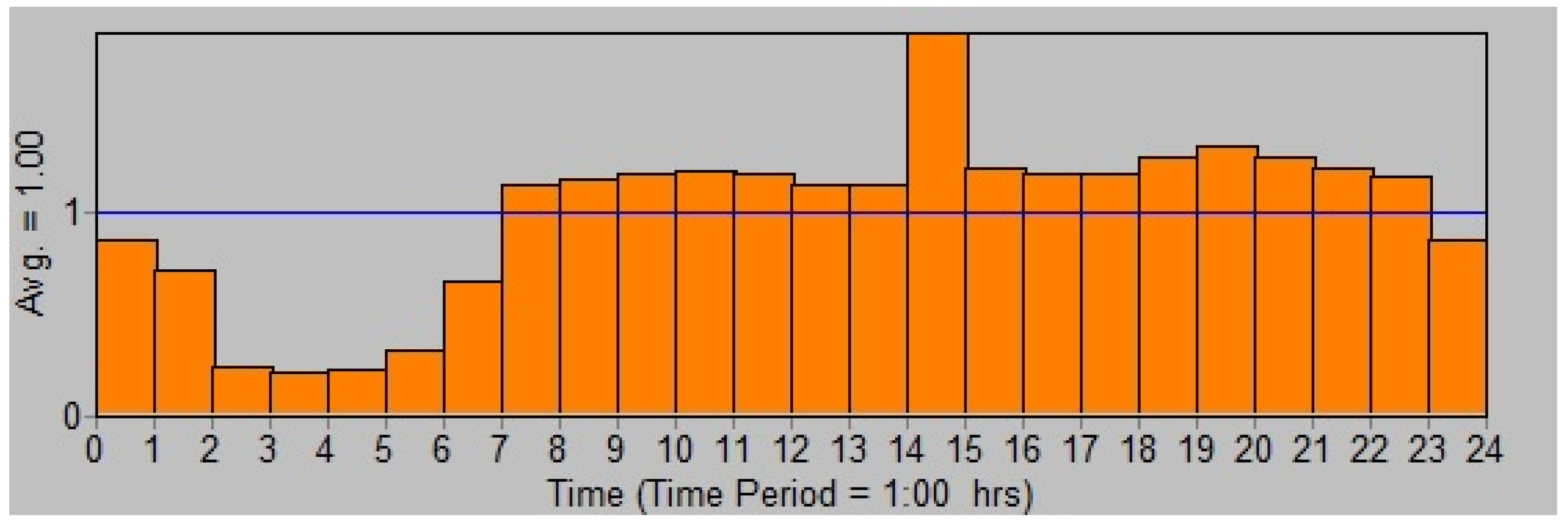
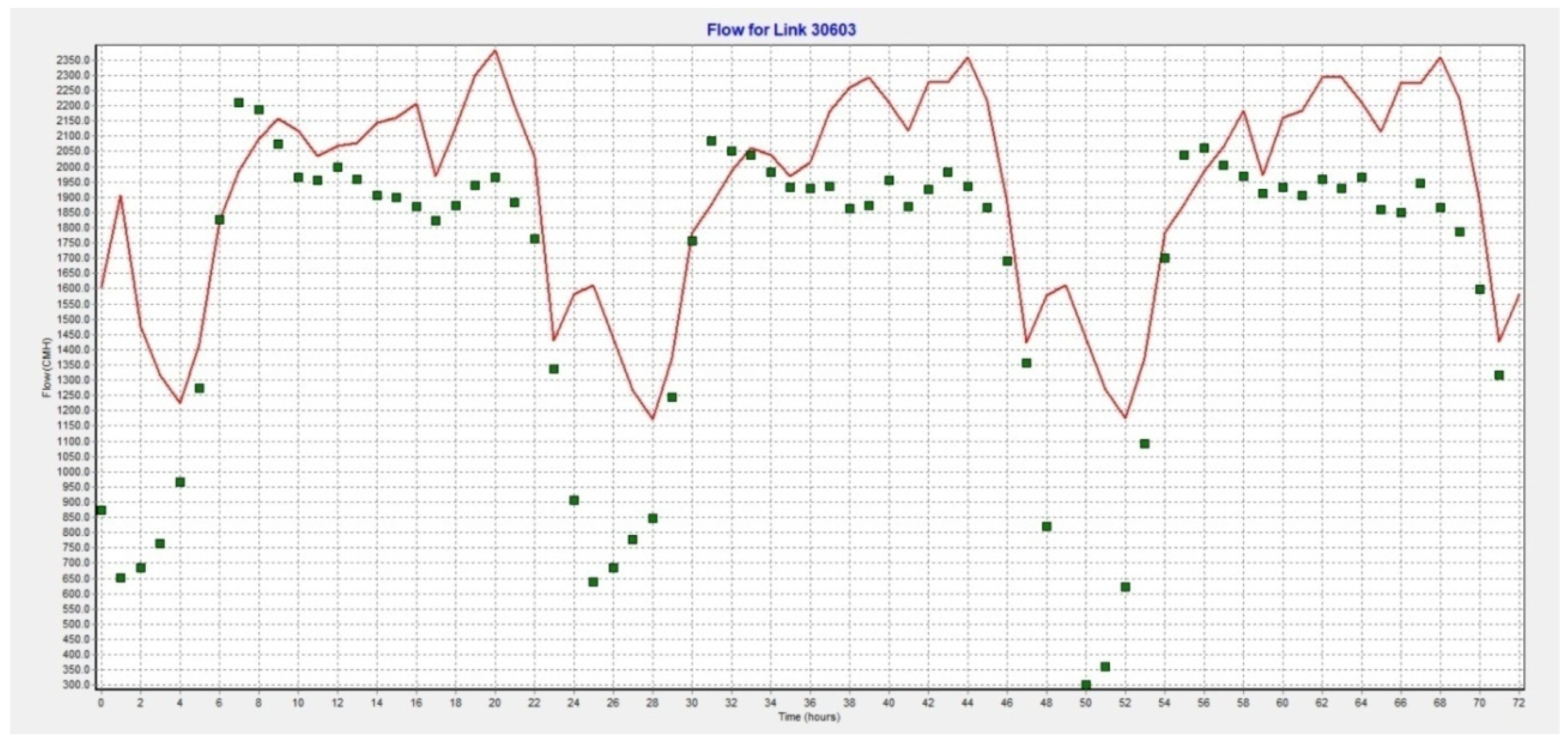
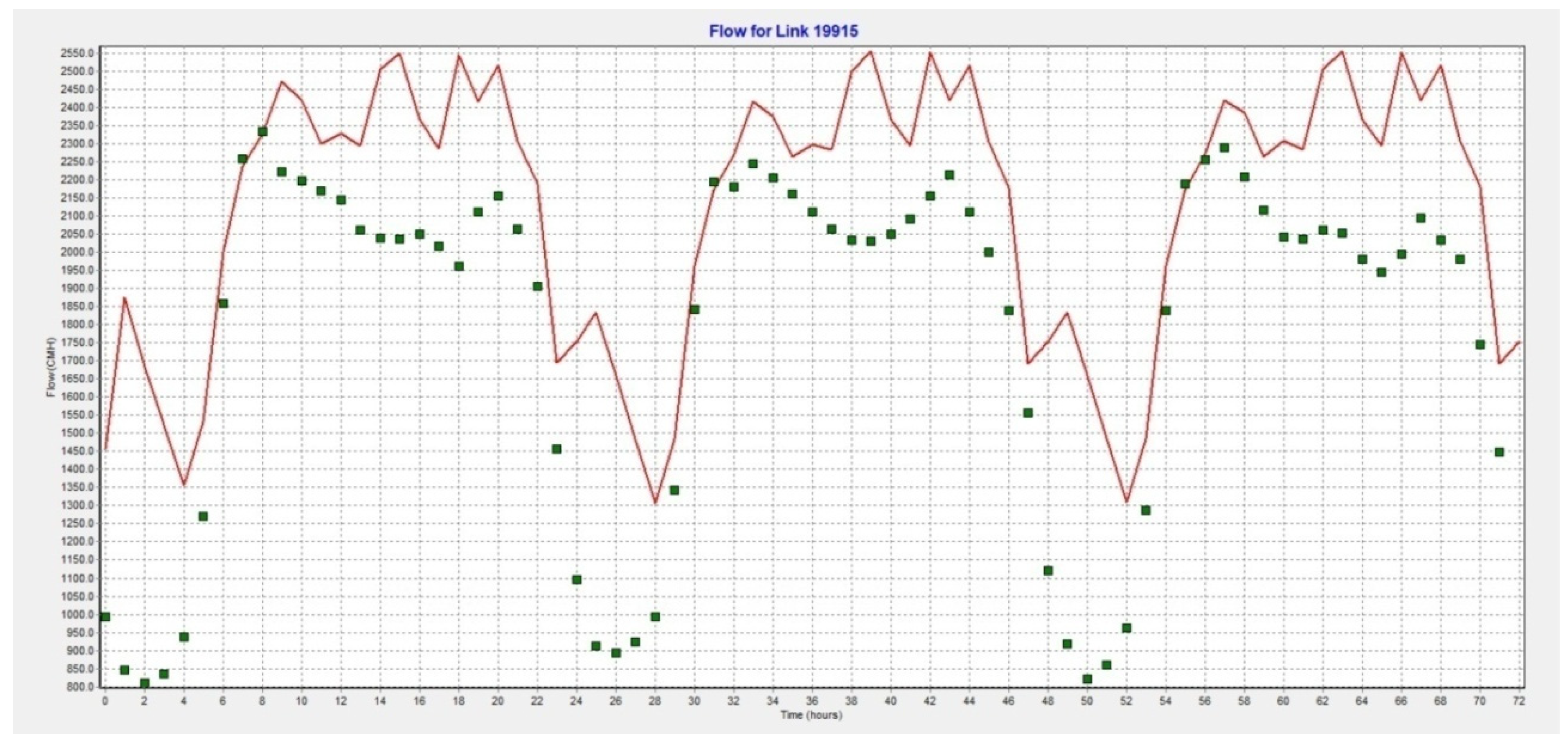
Industrial consumers often collect water irregularly or periodically, contributing to the maintenance of high network pressures around the clock at 75–100 m H₂O. Figure 4 and Figure 5 show exemplary water consumption patterns for industry, showing irregular water consumption. Figure 4 shows a customer receiving water for 13 h, and Figure 5 shows a customer characterized by a certain regularity of water intake from morning to night.

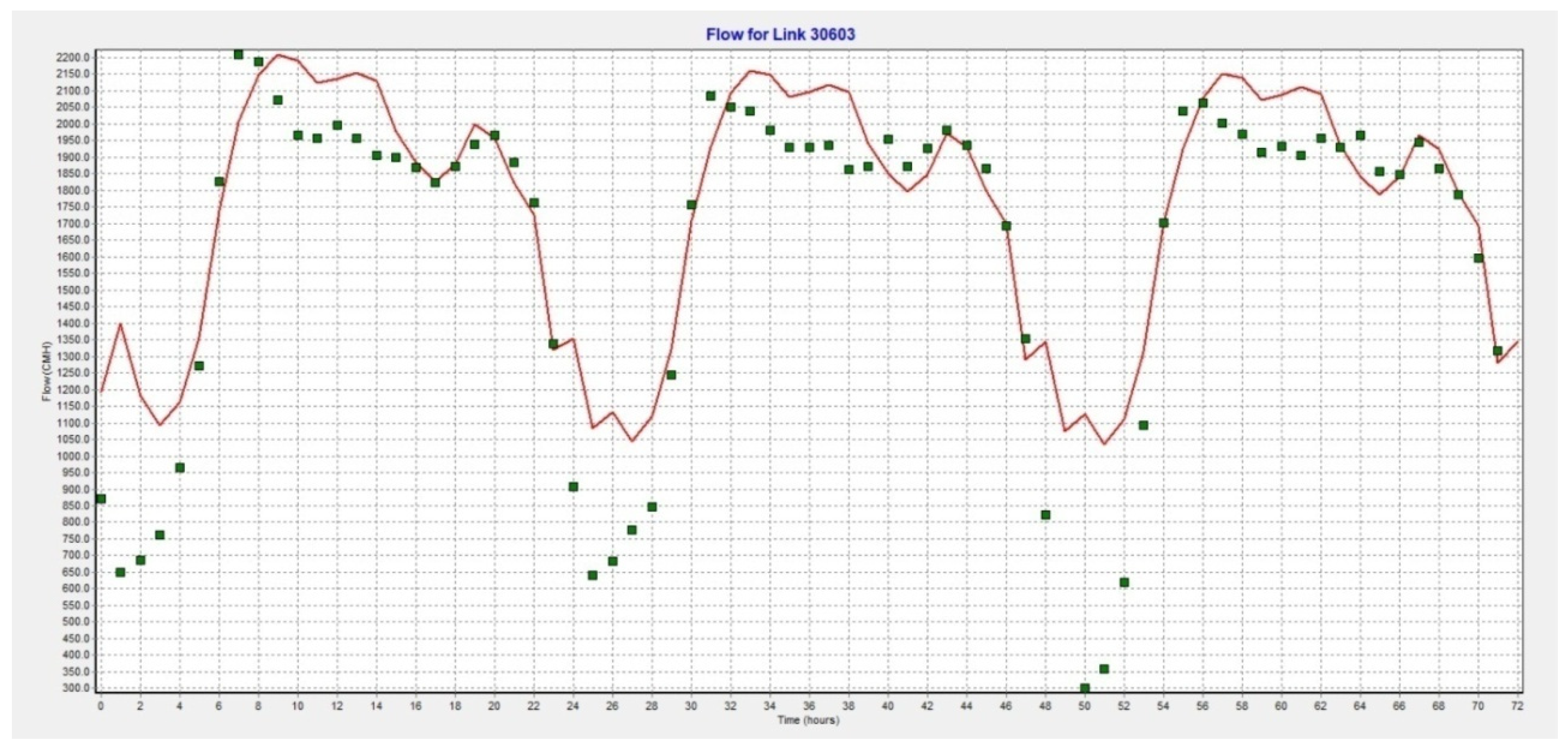
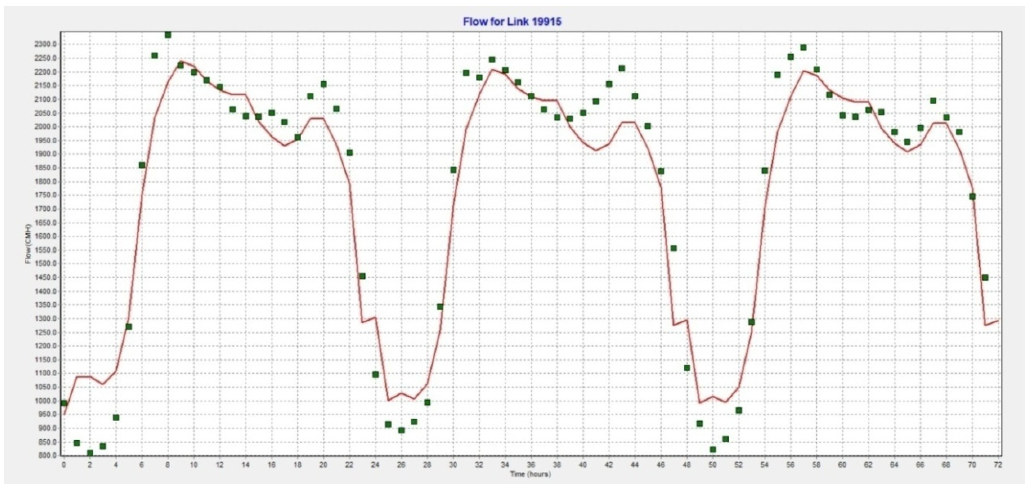
3. Assumptions Simulation and Result Discussion

A calibrated model was used in the study. EPANET 2.0 was used for the simulation. The network graph was exported from the GIS database, while the water demand data fora one-year period (2016) was exported from the available billing databases. Daily water consumption patterns were created from the SCADA telemetry system. The model was built from 1488 pipes and 1989 nodes, 524 valves, 22 pumps, 4 tanks and 4 reservoirs. The calibration was performed for data from a one-month period October 2016), while model validation covered a period of three days (17–19 October).Correlation of simulation results and actual measurements for flows was98.5% and was99.2%for pressure.

In the study, the model was simulated in three scenarios. For each scenario, data (average water demand and water consumption patterns) was retrieved from a different period:

1. Scenario I—simulation for one month (October); the period for which the model had been calibrated. In the simulation, there were267 nodes, with a total average water demand of 105,500 m³/day. Compatibility of the simulation result with the actual measurements for flows was98.5%, and for pressures 99.2%.

2. Scenario II—simulation for a period of 6 months (second half of 2016). In this simulation, there were275 nodal water demands with a total average water demand of 104,500 m³/day. Compatibility of the simulation result with the actual measurements for flowswas98.7%, and for pressures 99.3%.

3. Scenario III—Simulation for a period of one year (2016). In the simulation, there were281 nodal water demands with a total average demand of 123,900 m³/day. Compatibility of the model with the actual measurements for flows was97.5%, and for pressures 98.7%.

For each scenario, a different number of nodes with water demands was received, as well as a different value for water consumption. This could be caused by periodic water intake from some water consumption points, or by device failure. In relation to Scenario I, water demand for Scenario II was 1% lower, while for Scenario III it was 15% higher. This indicates that the length of the period, from which the data was exported, has a great influence on the specifics of the model.

Due to the size of the supplying area, a detailed analysis was conducted for Tanks E (Figure 1, color blue). Figure 6, Figure 7, Figure 8, Figure 9, Figure 10 and Figure 11 show simulation results for two flows from Tanks E—west and east directions.

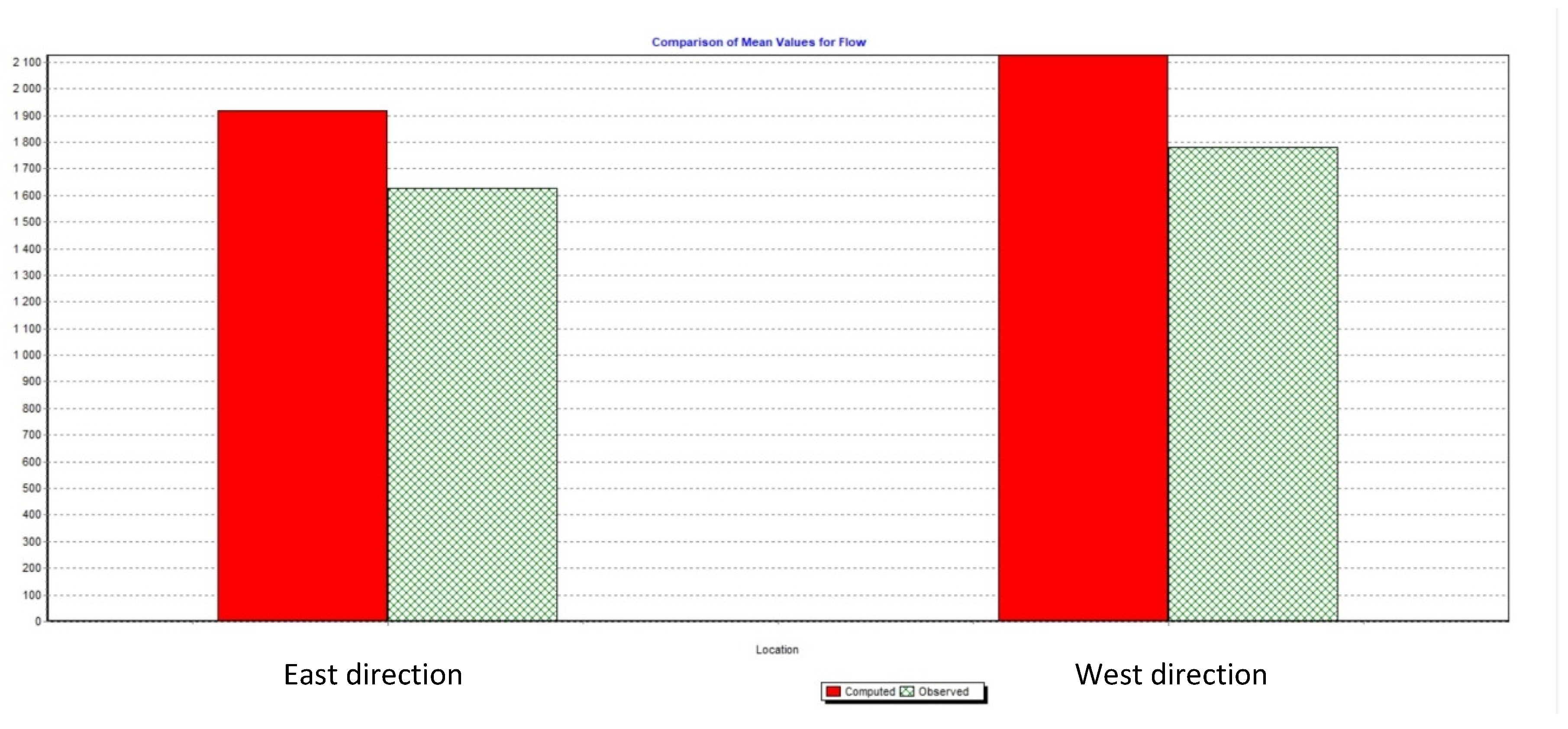
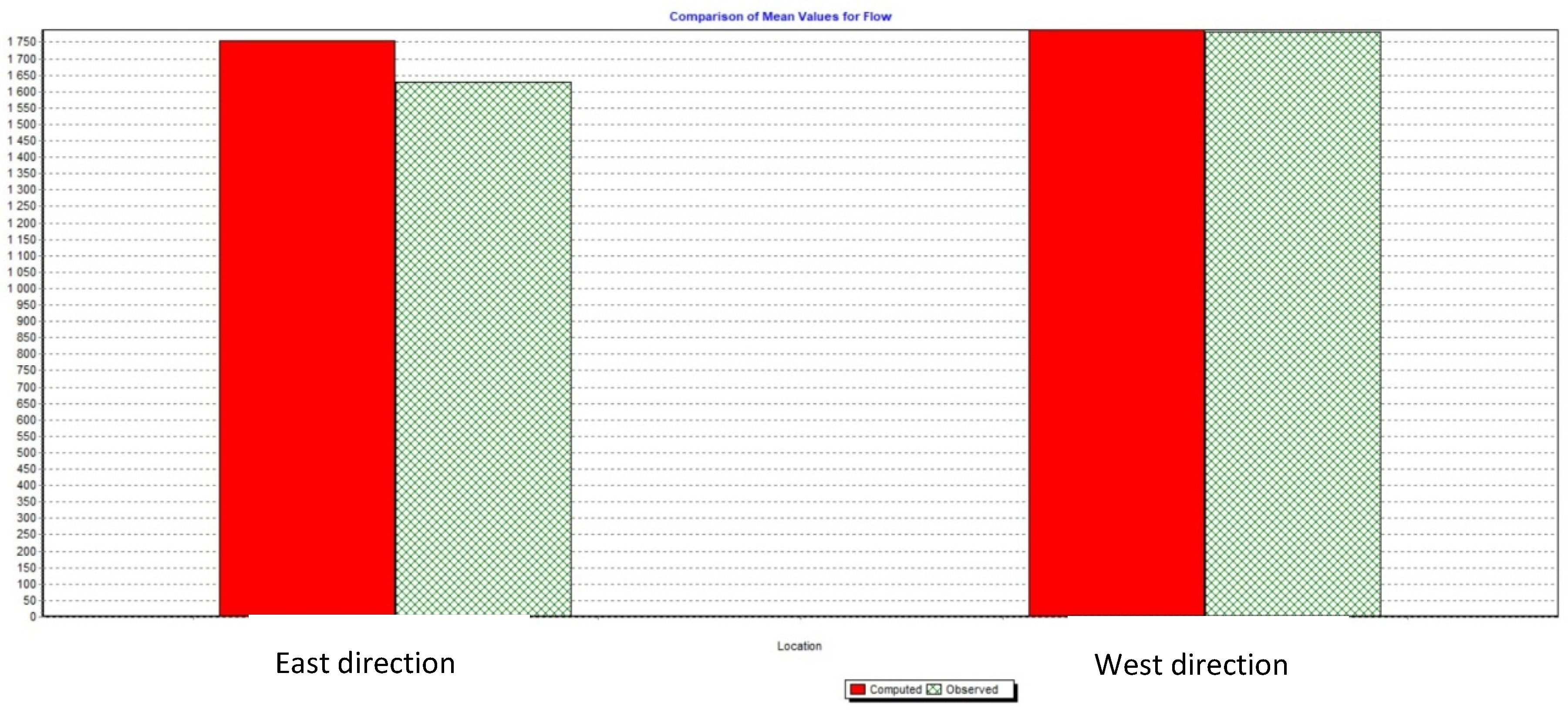
The best results were obtained for Scenario II (data from six months), and the worst for Scenario III (data from one year). Compatibility of simulation results for these two directions for mean flow values is as follows:

Scenario I: east direction 92.8%, west direction 99.6%

Scenario II: east direction 94.0%, west direction 98.6%

Scenario III: east direction 84.8%, west direction 83.8%.

Figure 12, Figure 13 and Figure 14 show charts of the comparison of mean values created in EPANET 2.0.

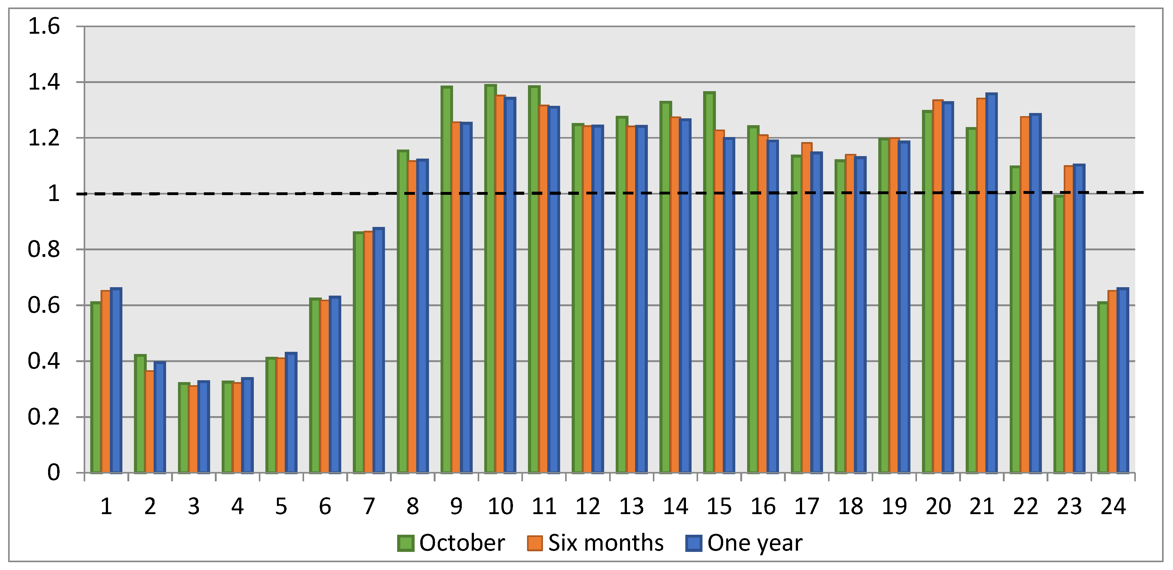
Such results may be due to various events occurring in the given periods, which could have influenced the quality of the data. The one-month period may seem appropriate because there are no seasonal fluctuations, but data from this period would be very sensitive to disturbances. In October, in this area, there were several pipe failures and several devices failures, which affected the data. In the six-month and one-year periods, there were dozens of such failures, but these distortions were “lost” in the correct data. On the other hand, the nodal demand values were calculated over the entire period, which contained seasonal fluctuations. This means that the average value could be overestimated or underestimated. The figures below show daily water consumption patterns for selected water intake points from the area supplied by Tanks E. Figure 15 shows the variability of the water consumption pattern, depending on the time period, for the domestic area, and Figure 16 for the industrial area. The graphs show that the longer the period from which the patterns were created, the closer the hourly demand values were to the daily average demand value (line = 1), meaning that they are more stable.

4. Conclusions

Calibration is a complex process that requires a lot of data analysis. Particular attention should be paid to water demand and water consumption patterns. These data are groups of information that are very sensitive to disturbances occurring during the considered period. Therefore, the period should not be too short or too long. In short periods, the water demand values may be overestimated or underestimated due to disturbances; while in extended periods, like one year, there are seasonal fluctuations that affect the data. Modelers should pay attention to the selected period, and should specify unwanted events such as pipe and devices failures. During modeling it is important to choose a period that reflects the normal operation of the WDS.