Abstract
Phytoplankton blooms are sporadic events in time and isolated in space. This complex phenomenon is produced by a variety of both natural and anthropogenic causes. Early detection of this phenomenon, as well as the classification of a water body under conditions of bloom or non-bloom, remains an unresolved problem. This research proposes the use of Inherent Optical Properties (IOPs) in optically complex waters to detect the bloom or non-bloom state of the phytoplankton community. An IOP index is calculated from the absorption coefficients of the colored dissolved organic matter (CDOM), the phytoplankton (φ) and the detritus (d), using the wavelength (λ) 443 nm. The effectiveness of this index is tested in five bloom events in different places and with different characteristics from Mexican seas: (1) Dzilam (Caribbean Sea, Atlantic Ocean) a diatom bloom (Rhizosolenia hebetata); (2) Holbox (Caribbean Sea, Atlantic Ocean) a mixed bloom of dinoflagellates (Scrippsiella sp.) and diatoms (Chaetoceros sp.); (3) Campeche Bay in the Gulf of Mexico (Atlantic Ocean) a bloom of dinoflagellates (Karenia brevis); (4) Upper Gulf of California (UGC) (Pacific Ocean) a diatoms bloom (Planktoniella sol) and (5) Todos Santos Bay, Ensenada (Pacific Ocean) a dinoflagellates bloom (Lingulodinium polyedrum). The diversity of sites shows that the IOP index is a suitable method to determine the bloom conditions.
1. Introduction
Phytoplankton blooms are sporadic events in time and isolated in space [1]. This complex phenomenon is produced by a variety of both natural and anthropogenic causes [2]. The availability of light and nutrients is a key factor for its development [3]. This factor is illustrated during the spring–summer period. At the beginning of this period, the seasonal increase in daily irradiation eliminates the light limitation, and the end of the thermal stratification supposes a supply of nutrients thanks to the turbulent and convective mixing processes, which allows the phytoplankton to grow rapidly [4]. However, phytoplankton blooms are not only limited to this period.
A bloom is the rapid growth of one or more species leading to an increase in the species’ biomass [5]. Different adjectives have been used to characterize the degree of negative impact of these blooms according to their characteristics and those of the causative species, such as toxic, noxious or harmful [6].
Identifying phytoplankton blooms has been the target of several researches [7,8,9,10]. Some research has focused on detecting changes in chlorophyll a fluorescence, changes in the composition of plankton species [9], or increases in nutrient levels [11]. Measuring the intensity of blooms has also been the subject of several researches, such as continuous measurements of fluorescence and chlorophyll a [12] deviations in normal biomass variations [13], the ratio of two in situ optical measurements such as chlorophyll fluorescence (Chl F) and optical particulate backscattering () [14], or satellite indices, such as the Maximum Chlorophyll Index (MCI) of the MERIS sensor [15].
Defining under which conditions an increase in phytoplankton biomass can be considered as a bloom is important to avoid the arbitrary use of the term bloom [4,7,16]. This research proposes the use of Inherent Optical Properties (IOPs), specifically the absorption coefficient, as an indicator that a phytoplankton community has passed into a bloom condition.
The absorption coefficient characterizes light absorption properties in the aquatic environment. Light absorption in natural waters is attributable essentially to four components: water, colored dissolved organic matter, photosynthetic biota and inorganic particles [17]. Thus, a (λ) can be expressed as:
where the subscripts w, cdom and p represent water, colored dissolved organic matter (CDOM) and particulate matter, respectively. This particulate material consists of phytoplankton (φ) and detritus (non-algal particles) (d), thus, [18].
Seawater components present a typical spectrum of light absorption, which means that they absorb light with a preference for certain wavelengths in the visible (400 to 700 nm) or ultraviolet (250 to 400 nm) [17]. Optically pure water absorbs light with a preference for red in the electromagnetic spectrum of 750 to 800 nm. Phytoplankton has an absorption spectrum characterized by two peaks located in the 440 and 675 nm spectrum, which are related to chlorophyll a absorption. Detritus and CDOM absorb with an exponential increase towards shorter wavelengths, with the most significant absorption towards the UV spectrum between 250 and 400 nm [19]. In optically complex waters, such as coastal and inland waters, the optical properties are determined by the combination of these water components in varying proportions [20].
The authors of [19] developed the IOP index with the objective of identifying phytoplankton blooms. This index is calculated from the absorption coefficients of the colored dissolved organic matter (CDOM), the phytoplankton (φ) and the detritus (d), using the wavelength (λ) 443 nm, and the relationship with chlorophyll a concentration and phytoplankton abundance is analyzed.
This research proposes the use of Inherent Optical Properties (IOPs) in optically complex waters to detect the bloom or non-bloom state of the phytoplankton community, as well as detecting whether it is an active or a decaying bloom. The objective is to test the effectiveness of the IOP index in bloom events in different coastal areas with distinctive characteristics.
2. Materials and Methods
2.1. Study Area
The study areas are well-known coastal areas of Mexico with distinctive characteristics where bloom events have been observed recurrently (Figure 1). These areas are as follows:
Area 1 is three coastal areas in the Yucatán Peninsula: Dzilam de Bravo (Dzilam for short) in the Yucatan state (Figure 1a), Holbox in the Quintana Roo state (Figure 1b), and Campeche Bay in the Campeche state (Figure 1c). This Peninsula is a karstic region, characterized by minimal soil cover and rapid infiltration of rain water, with the consequent high vulnerability of aquifer pollution [21,22]. The rainy season occurs from June through December with minimal rainfall occurring during the rest of the year. The unconfined Yucatán aquifer has submarine groundwater discharges (SGD) that can threat coastal ecosystems [22,23]. SGD has been linked to eutrophication and harmful algal blooms [23]. According to [24], the Yucatán coastal aquifer is a triple porosity system, where the flow of groundwater takes place mainly through interconnected cave systems and fractures, and drains inland catchment mainly through coastal springs. In recent years, intense coastal development is taking place within the Caribbean, due to tourism, which increases the risk of aquifer pollution. This development is particularly fast on the eastern coast of the Yucatan Peninsula (Quintana Roo state). Both Yucatán and Quintana Roo state coastal waters are influenced by waters of the Caribbean Sea and the Gulf of Mexico [25]. Campeche state coastal water is influenced by the current system of Yucatan/Lazo/Florida [26]. This region has a predominantly cyclonic circulation [27], caused by the wind effort [28], and by an upwelling on the north coast of the Yucatan Peninsula [29].
Area 2 is the Upper Gulf of California (UGC). The Gulf of California is a semi-enclosed sea in the Eastern Pacific. The UGC is located in the Northern Gulf of California, where the Sonora and Baja California state coasts intersect at a 60° angle [30]. It is considered as one of the most biologically productive marine regions [31,32], with peak chlorophyll a concentrations of 18.2 mg m−3 and averages of 1.8 mg m−3 between 1997 and 2007 in coastal waters near the delta [33]. This high productivity is due to a complex mix of factors, including coastal upwelling, wind-driven mixing, extreme tidal mixing and turbulence, thermohaline circulation, coastal-trapped waves, regular sediment resuspension, and, to a lesser extent, agricultural runoff, released nutrients from erosion of ancient Colorado River Delta sediments and groundwater discharges [31,34]. After the construction of the Hoover and Glen Canyon dams in the USA in 1935 and 1964, the Colorado river only discharges variable and insignificant surface water-flows occasionally into the Gulf of California [34].
Area 3, Todos Santos Bay (TSB), is a semi-enclosed bay, adjacent to the Pacific Ocean, within the upwelling zone of the Baja California peninsula (Mexico). This area is influenced by the California Current System (CCS), which produces coastal upwelling along the coast of the Baja California peninsula. This is a phenomenon with a marked seasonality caused by the prevailing winds from the northwest, which tend to be more intense during the spring and summer months [35,36,37]. Two water masses integrate the CCS, the California Current (CC), a year-round equatorward surface flow, which transports Subarctic Water (SAW), characterized by low salinity, and the California Undercurrent (CU), a poleward subsurface (100–400 m) flow that transports Equatorial Subsurface Water (ESsW), characterized by relatively high salinity, high nutrient concentration, and low dissolved oxygen content, according to a previous description [38]. SAW is mainly important during winter and spring, while ESsW appears at the end of summer and autumn [39]. In addition to the described seasonal variability, the El Niño-Southern Oscillation (ENSO) induces oceanographic changes in the region off Baja California at an interannual scale [39]. Altogether, these factors control primary productivity which is characteristically high [35,40]. Dinoflagellate algal bloom (DAB) events in this area have increased considerably in extension and frequency over the past two decades [41].
2.2. Collection of Samples
Water samples were taken in Mexico coastal waters at the stations shown in Figure 1. Samples were taken in four field campaigns, two in 2011 and two in 2017, during reported bloom events.
Dzilam (Yucatán) and Holbox (Quintana Roo) samples were collected between 27 and 30 August 2011 (nine and six samples respectively). All the Dzilam and Holbox stations were sampled at the surface (1.5 m); stations were selected based on reports of fishermen on fish mortality and patches of discolored water. Campeche Bay (Campeche) samples were collected between 22 and 24 September 2011 (19 samples). Campeche Bay was also sampled at the surface (1.5 m), except for stations number 13 and 16 which were sampled at 15 m. The campaign was conducted in response to a phytoplankton bloom reported by various local, state and federal public health institutions in Campeche. The Todos Santos Bay (TSB) in Ensenada (Baja California) was sampled on 2 June 2017 (seven samples) during the second week of a bloom event that lasted three weeks. This event was characterized by the bioluminescence observed during all the nights that lasted. TSB was also sampled at the surface (0.5 m). Stations 5, 6 and 7 were taken on the reddish patch that distinguished itself from the rest of the bay water.
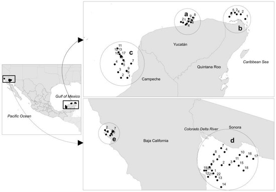
Figure 1.
Sampling stations. (a) Dzilam de Bravo (Yucatan); (b) Holbox (Quintana Roo); (c) Campeche Bay (Campeche); (d) Upper Gulf of California (Baja California and Sonora) and (e) Todos Santos Bay (Baja California).
These data were collected in small vessels where the samples were taken manually and stored in Nalgene dark bottles of high density polyethylene (HDPE) until processing in the laboratory. For the CDOM, samples were collected in amber glass bottles and refrigerated until laboratory processing.
Sampling of the Upper Gulf of California (UGC), was carried out from 23 February to 3 March 2017, on the research vessel “Tecolutla” of the Mexican Navy during the oceanographic cruise “Vaquita Marina 2017” (22 samples). Samples were taken with Niskin bottles attached to a rosette, and immediately processed in the vessel’s laboratory. Sampling depth was at the chlorophyll maximum fluorescence (10–40 m). The chlorophyll maximum was measured with an ECO FLNTU fluorimeter coupled to a CTD SB 19 Plus. During the oceanographic cruise, color patches were detected in the water; on this basis, it was decided to take samples.
In each study area, the samples were collected inside and outside the patches with evidence of a bloom, in order to be able to capture the variability that exists in a parcel of water, and to better define the baseline or mean of each campaign.
2.3. Absorption Coefficients Determination
The CDOM samples were filtered using a 0.2-μm pore membrane filter (Nuclepore™) and processed according to the methodology of [42]. The CDOM absorption coefficient, , was measured in the wavelength range of 250 to 800 nm in a 10-cm long quartz cuvette using Milli-Q water as reference.
The particulate matter absorption coefficient was determined using the methodology of [42]. A volume of seawater of 0.5 to 2 L, depending on the particle load, was filtered from water stored in Nalgene bottles, with Whatman GF/F glass fiber filters 25 mm in diameter and 0.7 μm in pore size. The particulate matter absorption coefficient, (), was measured in the wavelength range of 400 to 800 nm. Then, the filters are immersed in methanol to depigment the filter and obtain the detritus coefficient absorption, . The phytoplankton absorption coefficient, , was calculated by subtracting from .
The 2011 samples were read with a Perkin-Elmer Lambda 18 spectrophotometer, and the 2017 samples were read with a Cary 100 UV-Visible spectrophotometer.
A non-parametric one-way analysis of variance (Kruskal–Wallis) was performed to statistically assess variations in the absorption coefficients. The water absorption coefficient of phytoplankton, detritus and CDOM for each sampling area was compared.
2.4. IOP Index Determination
The IOP index was determined according to [19] following the next steps. Firstly, the absorption coefficients () were standardized, and a principal component analysis (PCA) was performed to explore associations between the sampled stations. Then, samples were classified as bloom or non-bloom using a factorial analysis [43]. Finally, the IOP index was calculated based on the first standardized empirical orthogonal function (SEOF1) [19] according to Equation (2).
The coefficients y are the eigenvalues resulting from the PCA, while and are the values obtained from the Pearson correlation matrix between the absorption coefficients. To describe the stages of a phytoplankton bloom [19], the values of the IOP index were interpreted as follows: (1) values in the interval (−1,1) show an average value and represent non-bloom conditions; (2) values in the interval (1,2) are above the average and represent decaying bloom conditions; and (3) values higher than 2 are anomalous and indicate active bloom conditions.
2.5. Phytoplankton Characterization
The blue/red ratio ( ) is an index that allows to characterize the dominant phytoplankton size [19,44,45,46,47]. It is calculated as expressed in Equation (3):
If the is >3.0, dominance of picophytoplankton (<2 μm) is implied. If the ratio is <2.5, dominance of microphytoplankton (>20 μm) is implied. Ratios between 2.5 and 3.0 indicate that there is no dominance of a particular group and it is identified as mixed bloom.
Some representative samples of each sampling were analyzed by microscopy to identify the main blooming species and/or genus. Samples were preserved in 125-mL bottles in a neutral lugol solution with a sodium acetate base in a 1:100 ratio. The samples were stored in dark and cold conditions until their identification. The Dzilam, Holbox, and Campeche samples were identified at the Florida Fish and Wildlife Conservation Commission (FWC). Phytoplankton identification was performed using an inverted Olympus IX71 microscope following a modified method of Utermöhl [48]. In the case of the UGC and TSB samples, the same method was performed using phase contrast microscopy with a microscopeBausch and Lomb; [49,50,51,52] were used as taxonomic references.
For Dzilam, Holbox and Campeche, the chlorophyll a concentration was determined fluorometrically on methanol extracts following the method of [53], using a Turner Designs 10-AU field fluorimeter.
3. Results and Discussion
In Table 1, we summarized the main characteristics of each bloom event. For each sampling campaign, we studied the contribution of each water component absorption coefficient (colored dissolved organic matter ( phytoplankton and detritus () to the global absorption coefficient at 443 nm. In Figure 2, the inner circumference shows the average contribution of each absorption coefficient to for each sampling campaign.

Table 1.
Characterization of bloom events. The absorption coefficient that contributes most to the Inherent Optical Properties (IOPs) is underlined for each sampling campaign.
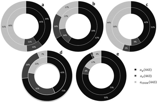
Figure 2.
Contribution of each absorption coefficient ( and ) to for each sampling area. The inner circumference shows the average contribution of each absorption coefficient to for each sampling campaign. The outer circumference represents the average value of sampling points classified as active bloom according to the IOP index. (a) Dzilam de Bravo (b) Holbox; (c) Campeche Bay; (d) Upper Gulf of California; (e) Todos Santos Bay.
In Dzilam, colored dissolved organic matter (CDOM) was the major contributor to . represented 48% of total absorption, followed by with 41% and with 11% (Figure 2a). In Holbox, phytoplankton was the major contributor to . represented 59% of water absorption, followed by with 27% and with 14% (Figure 2b). In Campeche Bay, as in Dzilam, the dominant absorption component was CDOM; was 50%, followed very closely by phytoplankton with 41% of , and a minor contribution of detritus ( was 9%) (Figure 2c). In the Upper Gulf of California, the highest contribution was from phytoplankton was 43%), followed by detritus ( was 35% of , and CDOM was 22%) (Figure 2d). In Todos Santos Bay (TSB), as in Holbox, phytoplankton represented the highest absorption percentage ( was 77%). However, in TSB, the contribution of CDOM and detritus is characteristically low (17% and 6% respectively).
In Figure 3, the phytoplankton, detritus and CDOM absorption spectrum of all sampling campaigns are compared. The phytoplankton absorption coefficient, , was significantly higher in TSB than in other sampling areas (p < 0.05 for (443)). No significant differences were observed between Dzilam and Campeche Bay (p > 0.05 for (443). The lowest values were observed in the UGC. The detritus absorption coefficient, , was significantly higher in the UGC than in all the other studied areas (p < 0.05 for ). No significant differences were observed between the Yucatan Peninsula areas (Dzilam, Holbox and Campeche), nor with TSB (p > 0.05 for ). The CDOM absorption coefficient, , was significantly higher in Dzilam and Campeche Bay than in other areas (p < 0.05 for ).
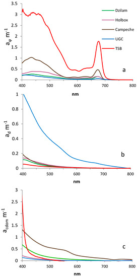
Figure 3.
Absorption coefficients (): (a) phytoplankton; (b) detritus and (c) colored dissolved organic matter (CDOM) of sampling points in active bloom for each sampling campaign (Dzilam, Holbox, Campeche Bay, Upper Gulf of California (UGC) and Todos Santos Bay (TSB)).
Figure 4 represents the absorption spectrum of each seawater component (phytoplankton, detritus and colored dissolved organic matter) for all the sampling points (Dzilam, Holbox, Campeche Bay, Upper Gulf of California and Todos Santos Bay). This graphical representation allowed us to compare the different study areas. In general terms, the most important components were phytoplankton and CDOM ( In this graph, we observed the significantly higher importance of detritus in the UGC. This detritus contribution is much more important near de Colorado River and decreases southward.
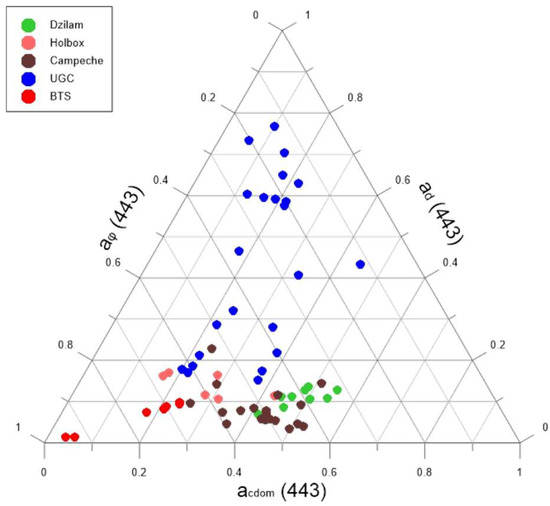
Figure 4.
Triangular diagram used to classify sampling points according to the contribution to of each component: phytoplankton ), colored dissolved organic matter ) and detritus ( ).
The IOP index was calculated from the absorption coefficients for each sampling area and sampling point. The IOP index results are represented graphically in Figure 5. In Figure 2, the outer circumference represents the average value of sampling points classified as active bloom according to the IOP index. In Dzilam, sampling points 4 and 6 had a value in the interval (1,2), meaning that they were above the sampling area average and in decaying bloom conditions. However, only sampling point 5 was above two and in active bloom conditions. In Figure 2a, we observed that the contribution of each absorption coefficient to in sampling point 5 is similar to the sampling campaign average. In Holbox, only sampling point 6 was above an IOP index value of two (Figure 5), and thus in active bloom conditions. In Figure 2b, we observed a higher contribution of phytoplankton to than the average value of the sampling campaign ( of 67% in sampling point 6 compared with 59% average value). The lower average contribution of phytoplankton when considering all sampling points was related with a higher CDOM contribution in non-bloom conditions. In Campeche Bay, sampling points 12, 14, 15 and 16 were in active bloom conditions (Figure 5). Sampling point 16 showed the highest anomaly; this sample was collected at 15 m depth. In Figure 2c, as in Holbox, we observed a higher contribution of phytoplankton to than the average value of the sampling campaign ( of 51% in sampling point 16 compared with 41% average value). The lower average contribution of phytoplankton was also related with a higher CDOM contribution in non-bloom conditions. In the Upper Gulf of California (UGC), sampling points 8, 19 and 22 were in decaying bloom conditions (IOP index value higher than one and lower than two), while sampling station 20 was in active bloom conditions according to the IOP index (Figure 5). In Figure 2d, we can observe that, as in Holbox and Campeche Bay, the contribution of phytoplankton to was higher than the average ( of 73% in sampling point 20 compared with 43% average value). In Todos Santos Bay, sampling point 6 was under decaying bloom conditions, while sampling point 7 was in active bloom conditions. As in Holbox and Campeche Bay, we noticed a higher contribution of phytoplankton to than the average value of the sampling campaign ( of 93% in sampling point 7 compared with 77% average value). The contribution of and was even lower than average.
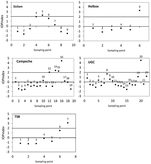
Figure 5.
IOP index results for each sampling campaign and sampling point. From top to bottom and from left to right: Dzilam, Holbox, Campeche Bay, Upper Gulf of California (UGC) and Todos Santos Bay (TSB).
In order to characterize the phytoplankton community, the blue/red ratio (B/R) is graphically represented in Figure 6. B/R values higher than 3 reveal a community dominated by picophytoplankton; B/R values lower than 2.5 reveal microphytoplankton (>20 µm) dominance; and B/R values between 2.5 and 3.0 indicate mixed community. In Dzilam, microphytoplankton dominated in the active bloom sampling point 5 ( = 1.71) (Figure 6). According to the microscope taxonomic analysis, the dominant species was the diatom Rhizosolenia hebetata. In Holbox, the ratio in active bloom point 6 was 2.57 (Figure 6), thus a mixed picophytoplanton and microphytoplankton community was observed. This was corroborated by microscope taxonomic analysis that identified the dinoflagellate Scrippsiella sp., and the diatoms Chaetoceros sp. and Rhizosolenia hebetata. In Campeche Bay, was lower than 2.5 in all active bloom condition points (Figure 6), so microphytoplankton was dominant. The dinoflagellate Karenia brevis was identified by microscopy as the dominant specie. In the UGC, was below 2.5 in nearly all the sampling stations (Figure 6). However, in sampling point 15, was 2.59, indicating a mixed community. The diatom Planktoniella sol was identified by microscopy. In Todos Santos Bay, was below 2.5 in sampling point 7 (active bloom conditions) (Figure 6), thus indicating microphytoplankton dominance. The most abundant species in this point was the dinoflagellate Lingulodinium polyedrum.
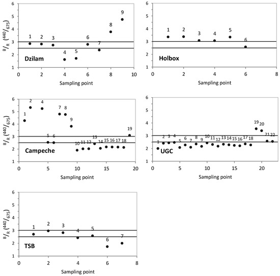
Figure 6.
Blue/red ratio (B/R) index for each sampling campaign and sampling point. From top to bottom and from left to right: Dzilam, Holbox, Campeche Bay, Upper Gulf of California (UGC) and Todos Santos Bay (TSB).
Dzilam (Yucatan), Holbox (Quintana Roo), and Campeche Bay (Campeche) (Figure 1a–c) are located in the karstic Yucatan Peninsula [54]. This region is characterized by rapid rain water infiltration into the groundwater system, and nearly no surface runoff [21,25]. Due to its hydrological characteristics, the lowest absorption coefficient is the detritus one ( is 11%, 14% and 9% respectively in each area) (Figure 3), as there is no relevant detritus source, no river runoff (the nearest one is located in south Campeche, far from the sampling area located in north Campeche). The climate of the region is characterized by three seasons associated with rainfall patterns: the dry season (March to May), the rainy season (June to October) and the northern wind season [55]. In this region, submarine groundwater discharges (SGDs) play a significant role in driving the nutrient stoichiometry (N:Si:P ratio) in receiving waters, which is a key factor in phytoplankton assemblages. SGDs are an important source of nitrogen, particularly , during the wet season (June to October), the high N:P ratio in SGDs can drive phosphorus limitation in the nearshore environment [23]. SGDs are also rich in silica, which can lead to diatom growth. Several studies have concurred that low salinity groundwater is an important source of nutrients in the Yucatan, specifically and silica, and have linked SGD sto harmful algal blooms [23]. According to [55], the HAB events in the state of Yucatan have been reported almost every year since 2001, covering an approximate area of 6000 km2.
Our sampling was developed during the large-scale pelagic HAB event of August–December, 2011. This event started in Dzilam and tended to move westward along the northern Yucatan coast [54]. In Dzilam, the dominance of the diatom Rhizosolenia hebetata can be explained by the input of silica from nearby springs (cenotes). The authors of [56] observed the the maximum chlorophyll a concentrations on 8 and 30 August. Our sampling was performed on 27 August. So, the degradation of phytoplankton cells from the previous peak may explain the high contribution of the CDOM absorption coefficient (48% on average). The sampling point identified as being in active bloom conditions according to the IOP index had significantly higher chlorophyll a levels, 12.5 mg m−3, which indicates non-bloom conditions—3.1 mg m−3 on average.
In Holbox, the diatoms Chaetoceros sp. and Rhizosolenia hebetata were also dominant, but dinoflagellates of Scrippsiella sp. were also abundant. Both Chaetoceros sp. and Scrippsiella sp. were also observed in Dzilam during this HAB event according to [56]. The characteristic springs (cenotes) of the Quintana Roo state could have supplied the silica needed for this sustained diatom bloom. Also in this sampling campaign, the sampling point identified as being in active bloom conditions according to the IOP index had significantly higher chlorophyll a levels, 12.5 mg−3, which indicates non-bloom conditions—2.2 mg m−3 on average.
In Campeche Bay, the blooming species was identified as the dinoflagellate Karenia brevis. Again, in this sampling campaign, the sampling point in active bloom conditions according to the IOP index had significantly higher chlorophyll a levels, 33.2 mg m−3, than sampling points in non-bloom conditions, 7.0 mg m−3 on average. The CDOM absorption coefficient, was as high as in Dzilam (higher than in all the other study areas) (Figure 3). Our sampling was performed on 22 September 2011. So, the high CDOM values could be explained by the degradation of accumulated phytoplankton cells during August and September. This region is influenced by the current system of Yucatan/Lazo/Florida [26]. It is important to note that even under very high CDOM values, the IOP index was able to distinguish an active phytoplankton bloom.
The Upper Gulf of California (UGC) and Colorado River Delta (CRD) area, is a region of sediment re-suspension characterized by high detritus levels, low light extinction coefficient values (−0.05 m−1) and high sedimentary loads (maximum values of 8 g/L) [30]. So, we expected the highest detritus absorption coefficient () to be observed. It is remarkable that, also under very high detritus levels, the IOP index was able to distinguish an active phytoplankton bloom.
In Todos Santos Bay (TSB), the most abundant species during our study was the dinoflagellate Lingulodinium polyedrum. The authors of [41] have reported an increase in dinoflagellate algal blooms (DABs), with Lingulodinium polyedrum as the dominant species, over the past few years in coastal areas off Baja California. Our sampling was developed on 2 June 2017, that is late spring, when L. polyedrum blooms usually occur in this area [41]. This blooms have been related with increases in irradiance, daylight hours, temperatures between 17 and 23 °C, stratification of the water column and formation of a seasonal surface thermocline [57]. These blooms are favoured by the convergence of surface currents and winds, which induce the transport of cells that tend to concentrate near the surface and toward the coast [41,58]. This bloom presented the highest phytoplankton absorption coefficient () observed in our study (Figure 3).
4. Conclusions
The selected study areas have allowed us to apply the IOP index within the wide variability of optically complex coastal waters. Within this variability, we found areas with dominance of detritus or CDOM, despite the samplings being developed in areas with observed phytoplankton blooms. The IOP index was able to discern sampling points in active bloom conditions from points in decaying bloom conditions. In the Yucatan region, the IOP index distinguished points in active bloom from points with high CDOM due to phytoplankton cell degradation from previous bloom. Also, the IOP index has been proved useful to distinguish phytoplankton blooms from the natural variability of one area. In the case of the UGC, typical high detritus levels produce a high absorption coefficient, which is not related with phytoplankton blooms. The IOP index was able to identify points in active bloom conditions from points with high detritus load.
To be able to distinguish a phytoplankton bloom from natural variability, regular monitoring is important. The inherent optical properties play a key role for correctly identifying phytoplankton blooms, but are highly variable in complex coastal waters. Different coastal areas have different baseline values that should be defined, thus enabling the detection of anomalous events. Thus, the measurement of absorption coefficients should be considered in programs monitoring coastal waters. The use of remote sensing can help to define IOPs from satellite reflectances, , and to build a baseline at a lower cost. Further research is needed to test whether contrasting in situ IOP measurements at baseline, calculated by remote sensing using the IOP index, are also able to correctly identify active phytoplankton blooms.
Acknowledgments
CONACYT supported this research with the doctoral grant, with announcement number 251025 of year 2015. The Generalitat Valenciana (Spain) provided funding through a scholarship for research staff to María-Teresa Sebastiá-Frasquet (BEST/2017/217).
Author Contributions
Jesús A. Aguilar-Maldonado carried out the tests and analyses developed in the article, drafted the text of the article and supported the sampling campaigns. Eduardo Santamaria-del-Ángel and Adriana G. Gonzalez-Silveira are authors of the methodology on which this article was based; the data used were obtained by resources of their research group, and they took part in the sampling campaigns. Maria-Teresa Sebastia-Fraquet organized the text, compiled and wrote data, and formulated new ideas for this article; she was also fundamental in the writing and correction of English. Omar D. Cervantes-Rosas, Lus M. López-Acuña, Angélica Gutiérrez-Magness collaborated in the entire process with ideas, corrections and advisory times.
Conflicts of Interest
The authors declare no conflict of interest. The founding sponsors had no role in the design of the study; in the collection, analyses, or interpretation of data; in the writing of the manuscript, and in the decision to publish the results.
References
- Gower, J.; King, S.; Borstad, G.; Brown, L. Detection of intense plankton blooms using the 709 nm band of the MERIS imaging spectrometer. Int. J. Remote Sens. 2005, 26, 2005–2012. [Google Scholar] [CrossRef]
- Carstensen, J.; Conley, D. Frequency, composition, and causes of summer phytoplankton blooms in a shallow coastal ecosystem, the Kattegat. Limnol. Oceanogr. 2004, 49, 191–201. [Google Scholar] [CrossRef]
- Legendre, L. The significance of microalgal blooms for fisheries and for the export of particulate organic carbón in oceans. J. Plankton Res. 1990, 12, 681–699. [Google Scholar] [CrossRef]
- Ji, R.; Edwards, M.; Mackas, D.; Runge, J.; Thomas, A. Marine plankton phenology and life history in a changing climate: Current research and future directions. J. Plankton Res. 2010, 32, 1355–1368. [Google Scholar] [CrossRef]
- Richardson, K. Harmful or exceptional phytoplankton blooms in the marine ecosystem. Adv. Mar. Biol. 1997, 31, 301–385. [Google Scholar]
- Smayda, T.J. What is a bloom? A commentary. Limnol. Oceanogr. 1997, 42, 1132–1136. [Google Scholar] [CrossRef]
- Brody, S.R.; Lozier, M.S.; Dunne, J.P. A comparison of methods to determine phytoplankton Bloom initiation. J. Geophys. Res. Oceans 2013, 118, 2345–2357. [Google Scholar] [CrossRef]
- Platt, T.; Fuentes-Yaco, C.; Frank, K.T. Spring algal Bloom and larval fish survival. Nature 2007, 423, 398–399. [Google Scholar] [CrossRef] [PubMed]
- Schneider, B.; Kaitala, S.; Maunula, P. Identification and quantification of plankton bloom events in the Baltic Sea by continuous pCO2 and chlorophyll a measurements on a cargo ship. J. Mar. Syst. 2006, 59, 238–248. [Google Scholar] [CrossRef]
- Gittings, J.A.; Raitsos, D.E.; Racault, M.F.; Brewin, R.J.; Pradhan, Y.; Sathyendranath, S.; Platt, T. Seasonal phytoplankton blooms in the Gulf of Aden revealed by remote sensing. Remote Sens. Environ. 2017, 189, 56–66. [Google Scholar] [CrossRef]
- Huppert, A.; Blasius, B.; Stone, L. A Model of Phytoplankton Blooms. Am. Nat. 2002, 159, 156–171. [Google Scholar] [CrossRef] [PubMed]
- Fleming, V.; Seppo Kaitala, S. Phytoplankton spring bloom intensity index for the Baltic Sea estimated for the years 1992 to 2004. Hydrobiologia 2006, 554, 57–65. [Google Scholar] [CrossRef]
- Carstensen, J.; Henriksen, P.; Heiskanen, A.-S. Summer algal blooms in shallow estuaries: Definition, mechanisms, and link to eutrophication. Limnol. Oceanogr. 2007, 52, 370–384. [Google Scholar] [CrossRef]
- Cetinic, I.; Perry, M.J.; D’Asaro, E.; Briggs, N.; Poulton, N.; Sieracki, M.E.; Lee, C.M. A simple optical index shows spatial and temporal heterogeneity in phytoplankton community composition during the 2008 North Atlantic Bloom Experiment. Biogeosciences 2015, 12, 2179–2194. [Google Scholar] [CrossRef]
- Alikas, K.; Kangro, K.; Reinart, A. Detecting cyanobacterial blooms in large North European lakes using the Maximum Chlorophyll Index. Oceanologia 2010, 52, 237–257. [Google Scholar] [CrossRef]
- Platt, T.; Sathyendranath, S.; White, G.; Fuentes-Yaco, C.; Zhai, L.; Devred, E.; Tang, C. Diagnostic properties of phytoplankton time series from remote sensing. Estuaries Coasts 2009, 33, 428–439. [Google Scholar] [CrossRef]
- Kirk, J.T.O. Light and Photosynthesis in Aquatic Ecosystems, 3rd ed.; Cambridge University Press: Cambridge, UK, 2011. [Google Scholar]
- Morel, A. Meeting the Challenge of Monitoring Chlorophyll in the Ocean from Outer Space. In Chlorophylls and Bacteriochlorophylls: Biochemistry, Biophysics, Functions and Applications; Grimm, B., Porra, R., Rüdiger, W., Scheer, H., Eds.; Springer: Dordrecht, The Netherlands, 2006; Volume 25, pp. 521–534. [Google Scholar]
- Santamaría-del-Angel, E.; Soto, I.; Millán-Nuñez, R.; González-Silvera, A.; Wolny, J.; Cerdeira-Estrada, S.; Cajal-Medrano, R.; Muller-Karger, F.; Cannizzaro, J.; Padilla-Rosas, Y.; et al. Experiences and Recommendations for Environmental Monitoring Programs. In Environmental Science, Engineering and Technology; Sebastia-Frasquet, M.-T., Ed.; Nova Science Publishers: Hauppauge, NY, USA, 2015; p. 32. [Google Scholar]
- IOCCG. Remote Sensing of Ocean Colour in Coastal, and Other Optically-Complex, Waters; Sathyendranath, S., Ed.; Reports of the International Ocean-Colour Coordinating Group: Dartmouth, NS, Canada, 2000. [Google Scholar]
- Hernández-Terrones, L.; Rebolledo-Vieyra, M.; Merrino-Ibarra, M.; Soto, M.; LeCossee, A.; Monroy-Rios, E. Groundwater pollution in karstic region (NE Yucatán): Baseline nutrient content and flux to coastal ecosystems. Water Air Soil Pollut. 2011, 218, 517–528. [Google Scholar] [CrossRef]
- Moore, Y.H.; Stoessell, R.K.; Easley, D.H. Fresh-Water/Sea-Water Relationship within a Ground-Water Flow System, Northeastern Coast of the Yucatan Peninsula. Ground Water 1992, 30, 343–350. [Google Scholar] [CrossRef]
- Hernández-Terrones, L.M.; Null, K.A.; Ortega-Camacho, D.; Paytan, A. Water quality assessment in the Mexican Caribbean: Impacts on the coastal ecosystem. Cont. Shelf Res. 2015, 102, 62–72. [Google Scholar] [CrossRef]
- Beddows, P.A.; Smart, P.L.; Whitaker, F.F.; Smith, S.L. Decoupled fresh-saline groundwater circulation of a coastal carbonate aquifer: Spatial patterns of temperature and specific electrical conductivity. J. Hydrol. 2007, 346, 18–32. [Google Scholar] [CrossRef]
- Herrera-Silveira, J.A.; Morales-Ojeda, S.M. Subtropical Karstic Coastal Lagoon Assessment, Southeast Mexico. The Yucatan Peninsula Case. In Coastal Lagoons: Critical Habitats of Environmental Change; CRC Press: Boca Raton, FL, USA, 2010; p. 26. [Google Scholar]
- Sánchez, F.J.; Gámez, D.; Guevara, G.; Shirasago, G.; Obeso, M. Análisis de la circulación superficial de mesoescala en la bahía de campeche mediante sensores activos y pasivos. Available online: http://www.ugm.org.mx/publicaciones/geos/pdf/geos10-1/sesiones_especiales/SE17.pdf (accessed on 21 January 2018).
- Monreal-Gómez, M.A.; Salas de León, D.A. Simulación de la circulación en la Bahía de Campeche. Geofís. Int. 1990, 29, 101–111. [Google Scholar] [CrossRef]
- Merrell, W., Jr.; Morrison, J. On the circulation of the western Gulf of Mexico with observations from April 1978. J. Geophys. Res. 1981, 86, 4181–4185. [Google Scholar] [CrossRef]
- Cochrane, J.D. Investigations of the Yucatan Current; the region of cold surface water. In Oceanography and Meteorology of the Gulf of Mexico; McLellan, H.J., Ed.; Annual Report; Texas A&M University: College Station, TX, USA, 1961; pp. 5–6. [Google Scholar]
- Carriquiry, J.D.; Sanchez, A. Sedimentation in the Colorado River delta and Upper Gulf of California after nearly a century of discharge loss. Mar. Geol. 1999, 158, 125–145. [Google Scholar] [CrossRef]
- Brusca, R.C.; Álvarez-Borrego, S.; Hastings, P.A.; Findley, L.T. Colorado River flow and biological productivity in the Northern Gulf of California, Mexico. Earth Sci. Rev. 2017, 164, 1–30. [Google Scholar] [CrossRef]
- Santamaría-del Ángel, E.; Millán-Núñez, R.; De la Peña, G. Efecto de la turbidez en la productividad primaria en dos estaciones en el Área del Delta del Río Colorado. Cienc. Mar. 1996, 22, 483–493. [Google Scholar]
- Daessle, L.W.; Orozco, A.; Struck, U.; Camacho-Ibar, V.F.; van Geldern, R.; Santamaría-del-Ángel, E.; Barth, J.A.C. Sources and sinks of nutrients and organic carbon during the 2014 pulse flow of the Colorado River into Mexico. Ecol. Eng. 2017, 106, 799–808. [Google Scholar] [CrossRef]
- Orozco-Durán, A.; Daesslé, L.W.; Camacho-Ibar, V.F.; Ortiz-Campos, E.; Barth, J.A.C. Turnover and release of P-, N-, Si-nutrients in the Mexicali Valley (Mexico): Interactions between the lower Colorado River and adjacent ground-and surface water systems. Sci. Total Environ. 2015, 512–513, 185–193. [Google Scholar] [CrossRef] [PubMed]
- Cepeda-Morales, J.; Durazo, R.; Millán-Nuñez, E.; De la Cruz-Orozco, M.; Sosa-Ávalos, R.; Espinosa-Carreón, T.L.; Soto-Mardones, L.; Gaxiola-Castro, G. Response of primary producers to the hydrographic variability in the southern region of the California Current System. Cienc. Mar. 2017, 43, 123–135. [Google Scholar] [CrossRef]
- Delgadillo-Hinojosa, F.; Camacho-Ibar, V.; Huerta-Díaz, M.A.; Torres-Delgado, V.; Pérez-Brunius, P.; Lares, L.; Castro, R. Seasonal behavior of dissolved cadmium and Cd/PO 4 ratio in Todos Santos Bay: A retention site of upwelled waters in the Baja California peninsula, Mexico. Mar. Chem. 2015, 168, 37–48. [Google Scholar] [CrossRef]
- Durazo, R.; Gaxiola-Castro, G.; Lavaniegos, B.; Castro-Valdez, R.; Gómez-Valdés, J.; Da, S.; Mascarenhas, A., Jr. Oceanographic conditions west of the Baja California coast, 2002–2003: A weak El Niño and subarctic water enhancement. Cienc. Mar. 2005, 31, 537–552. [Google Scholar] [CrossRef]
- Linacre, L.; Durazo, R.; Hernández-Ayón, J.M.; Delgadillo-Hinojosa, F.; Cervantes-Díaz, G.; Lara-Lara, J.R.; Camacho-Ibar, V.; Siqueiros-Valencia, A.; Bazán-Guzmán, C. Temporal variability of the physical and chemical water characteristics at a coastal monitoring observatory: Station Ensenada. Cont. Shelf Res. 2010, 30, 1730–1742. [Google Scholar] [CrossRef]
- Espinosa-Carreón, T.L.; Gaxiola-Castro, G.; Durazo, R.; De la Cruz-Orozco, M.E.; Norzagaray-Campos, M.; Solana-Arellano, E. Influence of anomalous subarctic water intrusion on phytoplankton production off Baja California. Cont. Shelf Res. 2015, 92, 108–121. [Google Scholar] [CrossRef]
- Millán-Núñez, E.; Macias-Carballo, M. Phytogeography associated at spectral absorption shapes in the southern region of the California current. CAlCOFI 2014, 55, 183–196. [Google Scholar]
- Gutierrez-Mejia, E.; Lares, M.L.; Huerta-Diaz, M.A.; Delgadillo-Hinojosa, F. Cadmium and phosphate variability during algal blooms of the dinoflagellate Lingulodinium polyedrum in Todos Santos Bay, Baja California, Mexico. Sci. Total Environ. 2016, 541, 865–876. [Google Scholar] [CrossRef]
- Mitchell, B.G.; Kahru, M.; Wieland, J.; Stramska, M. Determination of spectral absorption coefficients of particles, dissolved material and phytoplankton for discrete water samples. In Ocean Optics Protocols for Satellite Ocean Color Sensor Validation; NASA, Mueller, J.L., Fargion, G.S., Eds.; Flight Space Center: Greenbelt, MD, USA, 2002; Revision 3; Volume 3, pp. 231–257. [Google Scholar]
- Santamaría-del-Angel, E.; Millán-Núñez, R.; González-Silvera, A.; Callejas-Jiménez, M.; Cajal-Medrano, R.; Galindo-Bect, M. The response of shrimp fisheries to climate variability off Baja California, México. ICES J. Mar. Sci. 2011, 68, 766–772. [Google Scholar] [CrossRef]
- Stuart, V.; Sathyendranath, S.; Platt, T.; Maass, H.; Irwin, B.D. Pigments and species composition of natural phytoplankton populations: Effect on the absorption spectra. J. Plankton Res. 1998, 20, 187–217. [Google Scholar] [CrossRef]
- Lohrenz, S.E.; Weidemann, A.D.; Tuel, M. Phytoplankton spectral absorption as influenced by community size structure and pigment composition. J. Plankton Res. 2003, 25, 35–61. [Google Scholar] [CrossRef]
- Wu, J.; Hong, H.; Shang, S.; Dai, M.; Lee, Z. Variation of phytoplankton absorption coefficients in the northern South China Sea during spring and autumn. Biogeosci. Discuss. 2007, 4, 1555–1584. [Google Scholar]
- Millán-Nuñez, E.; Millán-Nuñez, R. Specific Absorption Coefficient and Phytoplankton Community Structure in the Southern Region of the California Current during January 2002. J. Oceanogr. 2010, 66, 719–730. [Google Scholar] [CrossRef]
- Utermöhl, H. Zur velvollkommung der quantitative phytoplankton-Methodik. Mitt. Int. Ver. Theor. Angew. Limnol. 1958, 9, 1–38. [Google Scholar]
- Haywood, A.J.; Steidinger, K.A.; Truby, E.W.; Bergquist, P.R.; Bergquist, P.L.; Adamson, J.; MacKenzie, L. Comparative morphology and molecular phylogenetic analysis of three new species of the genus Karenia (Dinophyceae) from New Zealand. J. Phycol. 2004, 40, 165–179. [Google Scholar] [CrossRef]
- Steidinger, K.A.; Wolny, J.L.; Haywood, A.J. Identification of Kareniaceae (Dinophyceae) in the Gulf of Mexico. Nova Hedwig. 2008, 133, 269–284. [Google Scholar]
- Gárate-Lizárraga, I.; Okolodkov, Y.; Cortés-Altamirano, R. Microalgas formadoras de florecimientos algales en el Golfo de California. In Florecimientos Algales Nocivos en México; García-Mendoza, E., Quijano-Scheggia, S.I., Olivos-Ortiz, A., Núñez-Vázquez, E.J., Eds.; CICESE: Ensenada, México, 2016; pp. 130–145. [Google Scholar]
- Quijano, S.I.; Barajas, M.; Chang, H.; Bates, S. The inhibitory effect of a non-yessotoxin-producing dinoflagellate, Lingulodinium polyedrum (Stein) Dodge, towards Vibrio vulnificus and Staphylococcus aureus. Rev. Biol. Trop. 2016, 64, 805–816. [Google Scholar] [CrossRef] [PubMed]
- Holm-Hansen, O.; Riemann, B. Chlorophyll a Determination: Improvements in Methodology. Oikos 1978, 30, 438–447. [Google Scholar] [CrossRef]
- Herrera-Silveira, J.A. Ecología de Los Productores Primarios en la Laguna de Celestún, México. Patrones de Variación Espacial y Temporal. Ph.D. Thesis, Universitat de Barcelona, Barcelona, Spain, 1993. [Google Scholar]
- Mendoza, M.; Ortiz-Pérez, M.A. Caracterización geomorfológica del talud y la plataforma continentales de Campeche-Yucatán, México. Investig. Geogr. 2000, 43, 7–31. [Google Scholar]
- Aguilar-Trujillo, A.C.; Okolodkov, Y.B.; Herrera-Silveira, J.A.; Merino-Virgilio, F.D.C.; Galicia-García, C. Taxocoenosis of epibenthic dinoflagellates in the coastal waters of the northern Yucatan Peninsula before and after the harmful algal bloom event in 2011–2012. Mar. Pollut. Bull. 2017, 119, 396–406. [Google Scholar] [CrossRef] [PubMed]
- Peña Manjarrez, J.; Gaxiola-Castro, G.; Helenes-Escamilla, J. Environmental factors influencing the variability of Lingulodinium polyedrum and Scrippsiella trochoidea (Dinophyceae) cyst production. Cienc. Mar. 2009, 35, 1–14. [Google Scholar] [CrossRef]
- Ruiz-de la Torre, M.C.; Maske, H.; Ochoa, J.; Almeda-Jauregui, C.O. Maintenance of Coastal Surface Blooms by Surface Temperature Stratification and Wind Drift. PLoS ONE 2013, 8, e58958. [Google Scholar] [CrossRef]
Publisher’s Note: MDPI stays neutral with regard to jurisdictional claims in published maps and institutional affiliations. |
© 2018 by the authors. Licensee MDPI, Basel, Switzerland. This article is an open access article distributed under the terms and conditions of the Creative Commons Attribution (CC BY) license (https://creativecommons.org/licenses/by/4.0/).