Entropy and Geometric Objects †


ACCESS e.V., Intzestr.5, D-52072 Aachen, Germany
†
Presented at the 4th International Electronic Conference on Entropy and Its Applications, 21 November–1 December 2017; Available online: http://sciforum.net/conference/ecea-4
Proceedings 2018, 2(4), 153; https://doi.org/10.3390/ecea-4-05007
Published: 20 November 2017
(This article belongs to the Proceedings of The 4th International Electronic Conference on Entropy and Its Applications)
Abstract
:Different notions of entropy can be identified in different communities: (i) the thermodynamic sense; (ii) the information sense; (iii) the statistical sense; (iv) the disorder sense; and (v) the homogeneity sense. Especially the “disorder sense” and the “homogeneity sense” relate to and require the notion of space and time. One of the few prominent examples relating entropy to geometry and to space is the Bekenstein-Hawking entropy of a Black Hole. Although being developed for the description of a physics object—a black hole—having a mass; a momentum; a temperature; a charge etc. absolutely no information about these attributes of this object can eventually be found in the final formula. In contrast; the Bekenstein-Hawking entropy in its dimensionless form is a positive quantity only comprising geometric attributes like an area A which is the area of the event horizon of the black hole-, a length LP—which is the Planck length-and a factor 1/4. A purely geometric approach towards this formula will be presented. The approach is based on a continuous 3D extension of the Heaviside function; with this extension drawing on the phase-field concept of diffuse interfaces. Entropy enters into the local; statistical description of contrast respectively gradient distributions in the transition region of the extended Heaviside function definition. The structure of the Bekenstein-Hawking formula eventually is derived for a geometric sphere based on mere geometric-statistic considerations.
1. Introduction
Different senses of entropy [1] lead to 5 different notions and perceptions of entropy: the Thermodynamic sense, the Information Sense, the Statistical Sense, the Disorder Sense, and the Homogeneity Sense.
Especially the “disorder sense” and the “homogeneity sense” relate to and require the notion of space and time. There is thus a need to introduce explicit spatial information into formulations of entropy.
In general the formulations of entropy used in statistical mechanics and information theory, however, do not comprise any explicit relation to space or time in the respective formulas. A prominent example actually relating entropy to geometry and space in is the Bekenstein-Hawking entropy of a Black Hole [2,3,4,5]. The entropy of a black hole has been described to base on microstates [6] indicating a microscopic origin.
The formulation of the entropy of a black hole plays an important role in the holographic principle [7,8,9] and in current entropic-gravity concepts [10,11] describing gravity as an emergent phenomenon.
Although being developed for the description of a physics object—a black hole—having a mass, a momentum, a temperature, a charge etc., absolutely no information about these attributes of this object can eventually be found in the final formula. In contrast, the Bekenstein-Hawking entropy SBH in its dimensionless form [12] is a positive quantity only comprising geometric attributes like an area A -which is the area of the event horizon of the black hole-, a length LP—which is the Planck length-and a factor 1/4:
Thus there might be a chance for purely geometric approach towards this formula. Such an approach is attempted in the present article. The approach is based on a continuous 3D extension of the Heaviside function and the phase-field method describing diffuse interfaces.
2. A Geometric Object
A 1-dimensional object is a line which is confined by a boundary consisting of two points. A 2-dimensional object can be defined as an area being confined by a boundary—the circumference—which is a line. A 3-dimensional object is a volume which also is confined by a boundary-its surface—which is an area. Any boundary distinguishes the object region of space from the “non-object” region. For an object with dimension n its boundary has the dimension n-1. Besides these two fundamental characteristics—bulk and boundary—(e.g., volume/surface, area/circumference, length/endpoints) geometric objects have no further physics attributes. Especially geometric objects do not have attributes like mass, charge, spin, and—further—they do not reveal any intrinsic structure. The following chapters for reason of simplicity and didactics will—without limiting the generality of the concept—limit the discussion to the case of a geometric sphere.
3. Sharp Interface Description of a Geometric Object
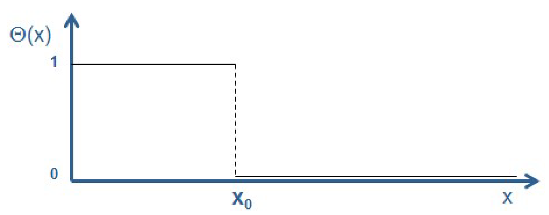
A common way to describe a sphere—or any other geometric object—is to use the Heaviside function Θ(x) [13], Figure 1:
The volume V of a sphere with radius r0 in spherical coordinates is then given by
with dΩ being the differential solid angle:
The Heaviside function cuts off any contributions of the integrand being larger than r0 and thus reduces the boundaries of the integral from infinity down to r0:
The surface of this sphere a can be calculated using the gradient of the Heaviside function. Gradients/derivatives of only appear—i.e., have non-zero values—at the positions r0 of the boundaries of an object. In fact, actually the definition of the Dirac delta function is based on the distributional derivative of the Heaviside function Θ(x) [14] as
Using Equation (5) the surface A of the sphere—and also the surface of more complex geometric objects—can easily be calculated as follows
This is the first term being relevant for the entropy of the black-hole—the area of the event horizon—i.e., the boundary making the black-hole distinguishable from the “non-black hole” or a “sphere” distinguishable from the “non-sphere”. The following sections aim to identify a way to derive or at least to provide reasoning for the other parameters i.e., for Lp and eventually for the factor ¼ on the basis of a description of a geometric sphere.
4. Phase-Field Description of a Geometric Object
Phase-field models [15,16] in the last decades have gained tremendous importance in the area of describing the evolution of complex structures like e.g., dendrites during phase-transitions. They even entered into materials engineering and process design tasks [17]. Similar to the Heaviside function Θ the phase-field Φ is a field describing the presence respectively the absence of an object, Figure 2.
In contrast to the Heaviside function being based on a mathematically sharp transition between the two states “1” and “0”, the phase field approach is based on a continuous transition between these two states within a transition width η. In case of a very narrow transition width, the phase-field function Φ(x) can be considered as a continuous, differentiable and 3D formulation of the Heaviside function Θ(x):
The shape of the transition in phase-field models depends on the choice of the potential in the model. A double-well potential e.g., leads to a hyperbolic-tangent profile while a double obstacle potential leads to a cosine profile of the Φ(x) function. However, nothing is a priori known neither about the type of potential nor about the shape of this function in the transition region also in phase-field models, Figure 3:
5. Entropy of Interfaces
General considerations about the shape of the phase-field function in the transition region between 0 and η (resp. between r0 and r0 + η) require continuity of both at the transition to the bulk regions i.e.,:
- is a small, non-zero, positive scaling constant having the unit of a length [L]
- has the dimension of an inverse length [L−1]
- defines the contrast between two regions. It is a dimensionless entity and takes values between 0 and 1
- Φ also has no physics units. It takes values between 0 and 1.
Especially “contrast” will take an important role throughout the following sections. From a philosophical/epistemological point of view, “contrast” provides the basis for any type of categorization or classification and thus the basis for any knowledge. From a physics/mathematics point of view its property of being a dimensionless variable seems very important as it can enter into the argument of the logarithm in this way.
5.1. Discrete Descriptions of the Entropy of an Interface
As a first step towards the description of the entropy of an interface, different models of crystal growth [18], the Jackson model, the Kossel crystal, and the Temkin model will be discussed in more detail. The interface between a solid and a liquid here serves as an instructive example for any type of transition between two different states.
The Jackson model [19] is used to describe the facetted growth of crystals. It assumes an ideal mixing of the two states (solid/liquid) in a single interface layer between the bulk states, Figure 4. The entropy of this interface layer in the Jackson model is described as an ideal mixing entropy being identical with the Shannon entropy of a binary information system:
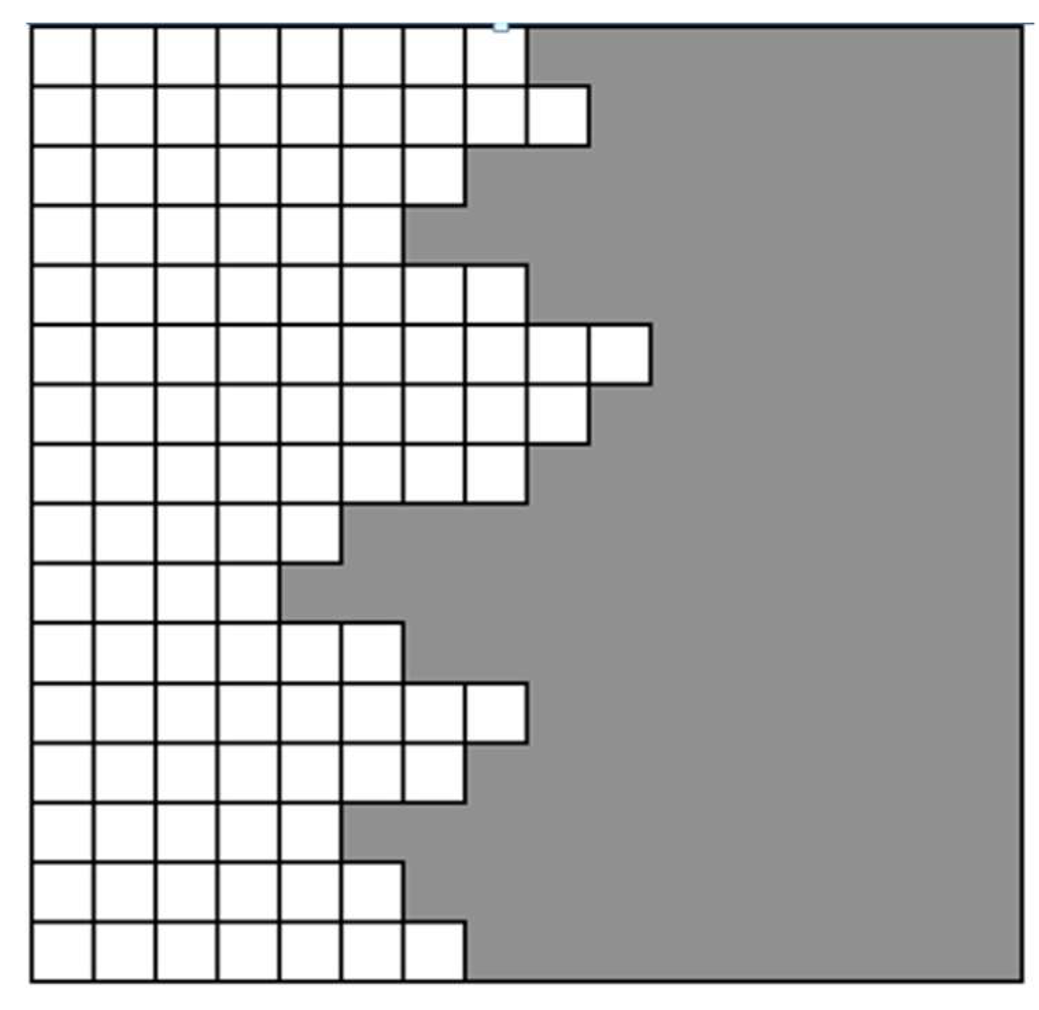
The Kossel model (see e.g., [18]) is a discrete model being used to describe the growth of crystals with diffuse interfaces, Figure 5. The Kossel model provides the basis for Temkin‘s discrete formulation of the entropy of a diffuse interface.
The Temkin model [20] is used to describe growth of crystals with diffuse interfaces. It assumes ideal mixing between two adjacent states/layers in a multilayer interface. The Temkin model describes the entropy of the diffuse interface as:
It basically allows for an infinite number of interface layers and recovers the Jackson model as a limiting case for a single interface layer. Accordingly it represents a more general approach.
Highlighting the importance of the Temkin model it can be stated that it introduces neighborhood relations between adjacent layers and thus an “order“ respectively a “disorder” sense. Most important, however, it obviously introduces a gradient and thus a length scale into the formulation of entropy. The gradient in the Temkin model is identified as follows:
with “l” being the distance between two adjacent layers and the gradient being assumed as constant between these two layers. Actually Temkin formulated his entropy using the contrast between adjacent layers. An extension of the Temkin model towards a continuous formulation and towards three dimensions is proposed in the next section.
5.2. From Discrete to Continuous
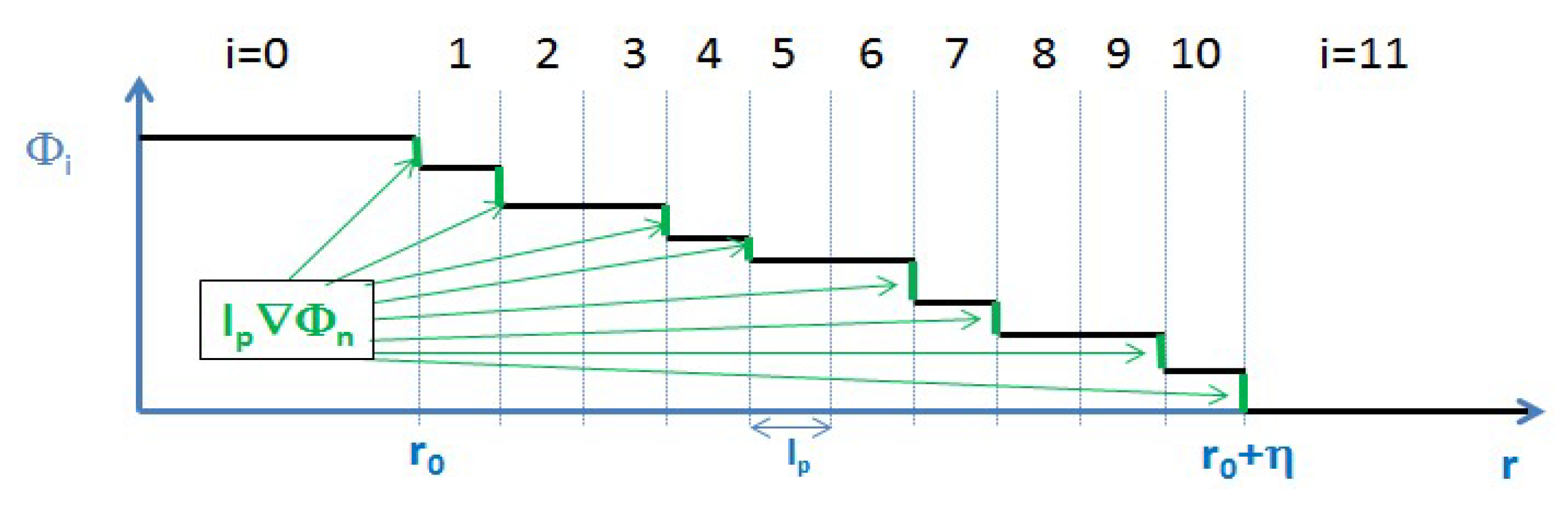
Temkin’s discrete formula for the entropy of a diffuse interface being described in the previous section can be visualized as follows, Figure 6:
The step towards a continuous formulation of Temkin’s entropy being already described elsewhere [21] corresponds to assuming an averaged and constant value of the gradient between each pair of cells. Variations of the gradient from cell to cell still remain possible. The number of cells may be infinite and the discretization length l may become extremely small. Some helpful relations read:
Making the step from discrete to continuous generates
Substituting
Making the same steps from 1 dimension to 3 dimensions in Cartesian coordinates means (i) extending the radial component product to the full scalar product and (ii) normalizing also the other integration directions by some discretization length:
Assuming isotropy of the discretization i.e.,
eventually leads to
The term
can be interpreted as an entropy density.
Switching back to spherical coordinates then yields:
Assuming isotropy (i.e., no dependence of Φ on angular coordinates) allows for integration over the solid angle dΩ
Terms with finite—i.e. non zero- values of the ∇Φ yielding contributions to the integral will only occur at the interface. Proportionality between the ∇Φ containing terms and the δ-function can thus be assumed for very small transition widths η of the phase-field Φ:
This proportionality can be formulated as an equation by introducing a hitherto unknown constant
This equation will be further discussed in the following chapter. Preliminarily inserting this relation into Equation (22) yields
This brings the formulation a step closer to revealing the same structure as the Bekenstein-Hawking entropy. The final step of identifying the factor ¼ is described in the following section.
6. Gradients in Diffuse Interfaces
The considerations about in the Temkin model highlighted the importance of gradients respectively of contrast for the formulation of the entropy of a diffuse interface. Nothing is by now specified about the exact shape of resp. the radial component of the gradient vector in spherical coordinates ∇rΦ.
In a first approximation ∇rΦ, could be a constant denoting the average gradient between 0 and η (see the blue dotted line in Figure 7). The calculation of the value of this average gradient in a discrete, spatial formulation reads
with the number N of the intervals discretizing the interface being defined as
This simple approach does however not match the continuity requirements for the gradient at the contact points to the bulk regions. It further leads to a statistically improbable, extremely sharp distribution of the contrast, see the blue bar in the histogram in Figure 7.
The average contrast being calculated from an entropy type distribution of contrast reads
The minimum gradient in the distribution has the value 0 (or may be finite but very small; see discussion section) while the maximum gradient is 1/lp. This allows fixing the boundaries of the integrals to 0 and 1.
which with
yields
When integrating over the interval [0,1] this integral interestingly yields a value of −¼:
The average gradient resp. the average contrast resulting from averaging the distribution thus reads
Replacing the contrast distribution by its average value i.e., approximating
then yields:
This eventually leads to
and thus finally to an expression for the entropy of a geometric sphere SGS revealing the samestructure as the Bekenstein-Hawking entropy of a black hole:
7. Summary and Discussion
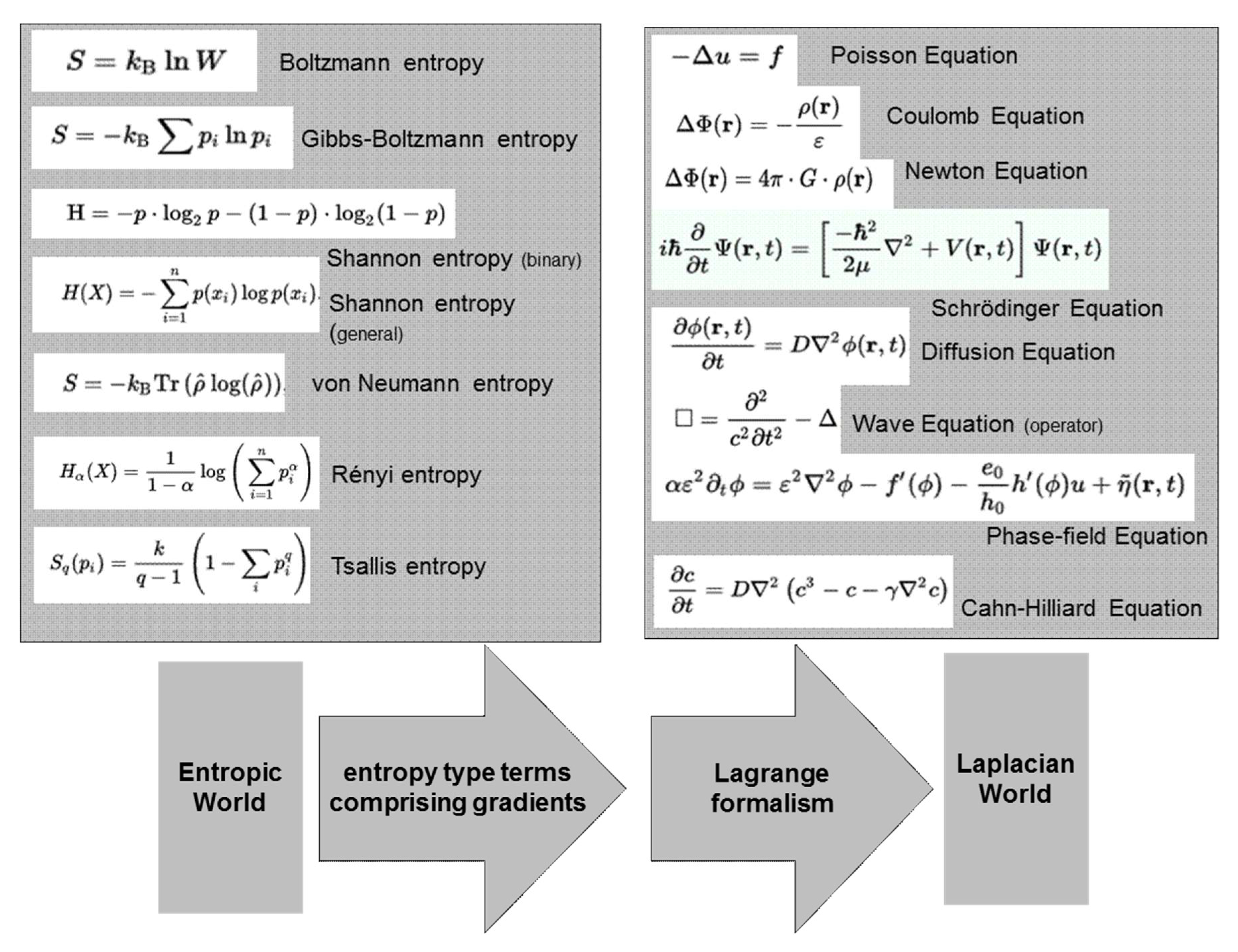
The structure of the Bekenstein-Hawking formula for the dimensionless entropy of a black hole has been derived for the case of a geometric sphere. This derivation is based only on geometric considerations. The key ingredient to the approach is a statistical description of the transition region in a Heaviside resp. a phase-field function. Based on the Temkin entropy of a diffuse interface gradients are introduced in form of scalar products into the formulation of entropy for this purpose. This introduces a length scale into entropy and provides a link between the world of entropy type models and the world of Laplacian type models, Figure 8.
The length being used as the smallest discretization length or as the inverse of the maximum gradient between two states reveals similar characteristics as the Planck length
The minimum gradient—being set to 0 when making the transition from Equation (28) to Equation (29)—may actually be a finite positive, but nonzero value being calculated as 1/Rmax with Rmax being some characteristic maximum length over which the transition from 1 to 0 occurs. This Rmax might be the radius of the sphere or the radius of the universe outside the sphere. Equation (33) in this case would contain additional terms leading to minor but perhaps important corrections of the factor 1/4:
Such corrections become important (i.e., reach the few % region) if the ratio of lp/Rmax gets close to 0.1 and might be subject to further discussions. The major implication of the entropy formulation comprising scalar products respectively gradients, however, is its perspective of providing a link between entropy type models and Laplacian type model equations as outlined in the final section.
8. Outlook
Bridging the gap between statistics/entropy type models and spatio-temporal models of the Laplacian world will lead to most interesting physics and new insights—e.g., on entropic gravity-may emerge when applying and exploiting the proposed “contrast-concept” in more depth.
First application of this concept [23] already allowed deriving the Poisson equation of gravitation including terms being related to the curvature of space. The formalism further generated terms possibly explaining nonlinear extensions known from modified Newtonian dynamics approaches.
Acknowledgments
The ideas being documented in the present article have emerged over several years in parallel to ongoing projects being funded by various institutions. A number of stimulating impulses arose from recent discussions about metadata, semantics, ontology, model classifications and other topics in the frame of the European Materials Modelling Council (EMMC-CSA project) being funded by the European Commission under grant agreement n° 723867.
Conflicts of Interest
The author declares no conflict of interest. The founding sponsors had no role in the design of the study; in the collection, analyses, or interpretation of data; in the writing of the manuscript, and in the decision to publish the results.
References
- Haglund, J.; Jeppsson, F.; Strömdahl, H. Different Senses of Entropy—Implications for Education. Entropy 2010, 12, 490–515. [Google Scholar] [CrossRef]
- Bekenstein, J.D. Black Holes and Entropy. Phys. Rev. D 1973, 7, 2333. [Google Scholar] [CrossRef]
- Hawking, S.W. The quantum mechanics of black holes. Sci. Am. 1977, 236, 34–40. [Google Scholar] [CrossRef]
- Bekenstein, J.D. Black-hole thermodynamics. Phys. Today 1980, 33, 24–31. [Google Scholar] [CrossRef]
- Bekenstein, J.D. Black holes and information theory. Contemp. Phys. 2004, 45, 31–43. [Google Scholar] [CrossRef]
- Strominger, A.; Vafa, C. Microscopic origin of the Bekenstein-Hawking entropy. Phys. Lett. B 1996, 37, 99–104. [Google Scholar] [CrossRef]
- Gerard, H. Dimensional Reduction in Quantum Gravity. arXiv 1993, arXiv:gr-qc/9310026. [Google Scholar]
- Bousso, R. The holographic principle. Rev. Mod. Phys. 2002, 74, 825–874. [Google Scholar] [CrossRef]
- Bekenstein, J.D. Information in the holographic universe. Sci. Am. 2003, 289, 58–65. [Google Scholar] [CrossRef] [PubMed]
- Verlinde, E.P. On the Origin of Gravity and the Laws of Newton. J. High Energy Phys. 2011, 29, 1–17. [Google Scholar] [CrossRef]
- Verlinde, E.P. Emergent Gravity and the Dark Universe. arXiv 2016, arXiv:1611.02269. [Google Scholar] [CrossRef]
- Bekenstein, J.D. Bekenstein-Hawking entropy. Scholarpedia 2008, 3, 7375. [Google Scholar] [CrossRef]
- Heaviside Step Function. Available online: https://en.wikipedia.org/wiki/Heaviside_step_function (accessed on 10 November 2017).
- Heaviside Step Function. Available online: https://en.wikipedia.org/wiki/Heaviside_step_function (accessed on 10 November 2017).
- Provatas, N.; Elder, K. Phase-Field Methods in Materials Science and Engineering; Wiley VCH: Weinheim, Germany, 2010. [Google Scholar]
- Steinbach, I. Phase-field models in Materials Science-Topical Review. Model. Simul. Mater. Sci. Eng. 2009, 17, 073001. [Google Scholar] [CrossRef]
- Schmitz, G.J.; Böttger, B.; Eiken, J.; Apel, M.; Viardin, A.; Carré, A.; Laschet, G. Phase-field based simulation of microstructure evolution in technical alloy grades. Int. J. Adv. Eng. Sci. Appl. Math. 2010, 2, 126–129. [Google Scholar] [CrossRef]
- Woodruff, D. The Solid Liquid Interface; Cambridge University Press: Cambridge, UK, 1973. [Google Scholar]
- Jackson, K.A. Liquid Metals and Solidification; ASM: Cleveland, OH, USA, 1958. [Google Scholar]
- Temkin, D.E. Crystallization Processes; Sirota, N.N., Gorskii, F.K., Varikash, V.M., Eds.; English Translation; Consultants Bureau: New York, NY, USA, 1966. [Google Scholar]
- Schmitz, G.J. Thermodynamics of Diffuse Interfaces. In Interface and Transport Dynamics; Emmerich, H., Nestler, B., Schreckenberg, M., Eds.; Springer Lecture Notes in Computational Science and Engineering; Springer: Berlin/Heidelberg, Germany, 2003; pp. 47–64. [Google Scholar]
- Bronstein, I.N.; Mühlig, H.; Musiol, G.; Konstantin, A. Semendjajew: Taschenbuch der Mathematik (Bronstein); Deutsch, H., Ed.; Verlag: Harri Deutsch, Germany, 2016. [Google Scholar]
- Schmitz, G.J. A combined entropy/phase-field approach to gravity. Entropy 2017, 19, 151. [Google Scholar] [CrossRef]
Figure 1.
Scheme of the Heaviside function Θ(x). This function takes the value 1 wherever the object/sphere is present and 0 else.
Figure 1.
Scheme of the Heaviside function Θ(x). This function takes the value 1 wherever the object/sphere is present and 0 else.

Figure 2.
Scheme of the phase-field function Φ(x). This function takes the value 1 wherever the object/sphere is present and 0 else. In contrast to the Heaviside function it reveals a continuous transition over a finite—though very small—interface thickness η.
Figure 2.
Scheme of the phase-field function Φ(x). This function takes the value 1 wherever the object/sphere is present and 0 else. In contrast to the Heaviside function it reveals a continuous transition over a finite—though very small—interface thickness η.
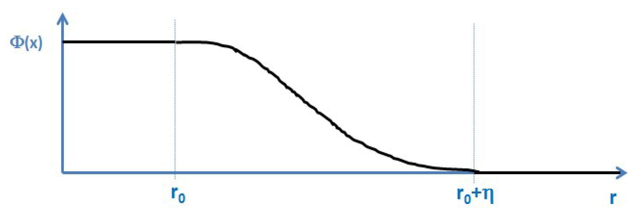
Figure 3.
Nothing is a-priori known about the shape of the functions in the small transition width between the two states. It should be noted that two state systems have a major importance also in quantum mechanical systems and transitions.
Figure 3.
Nothing is a-priori known about the shape of the functions in the small transition width between the two states. It should be noted that two state systems have a major importance also in quantum mechanical systems and transitions.
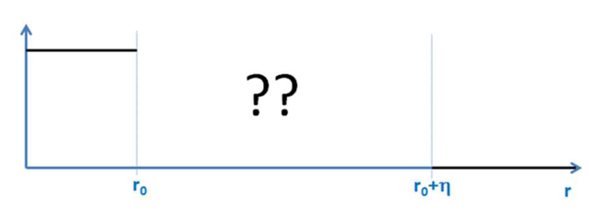
Figure 4.
The entropy distribution of the Jackson model generates Φ = 0.5 as the most probable value in the interface region.
Figure 4.
The entropy distribution of the Jackson model generates Φ = 0.5 as the most probable value in the interface region.
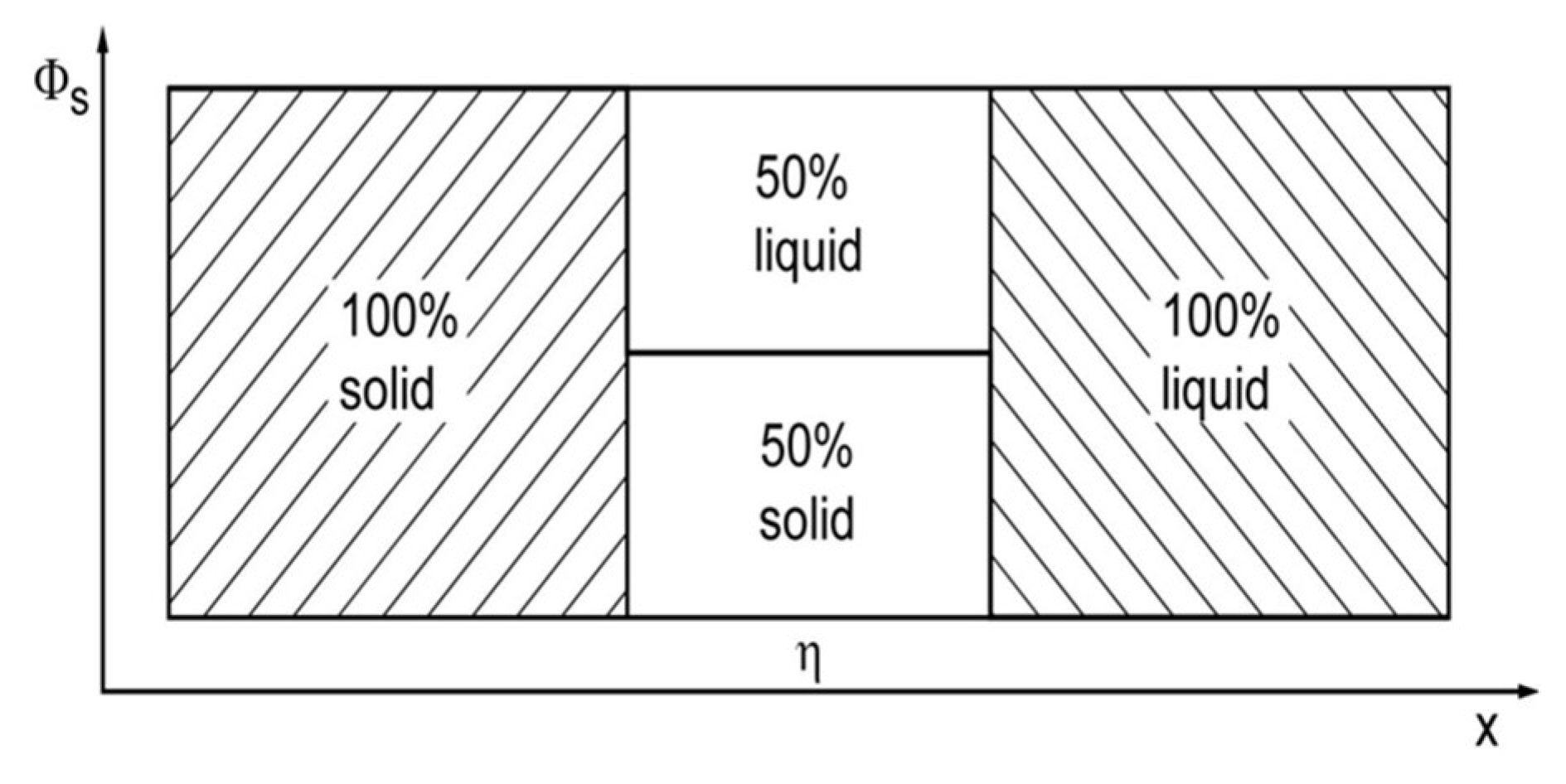
Figure 5.
The Kossel model assumes attachment of solid on existing solid only i.e., it does not allow for any overhang. Using multiple layers it describes a stepwise transition from 100% solid (the 4 left layers) to 100% liquid (from layer 11 to the right). The projection of layers 5 to 10 yields a decreasing fraction of solid with increasing layer number.

Figure 6.
The values of the Temkin model visualized as contrast i.e., (in green).

Figure 7.
Possible shapes of the Φ function in the transition region: A constant average gradient (blue) leads to an extremely narrow distribution of contrast being centered around lp/η. The green shapes lead to high counts for small contrast. The red shape leads to a broad distribution of small and high contrast values. An entropy type distribution of contrast xi (N = 10): H(x) = −10xln(x) is indicated as the red-line overlay.
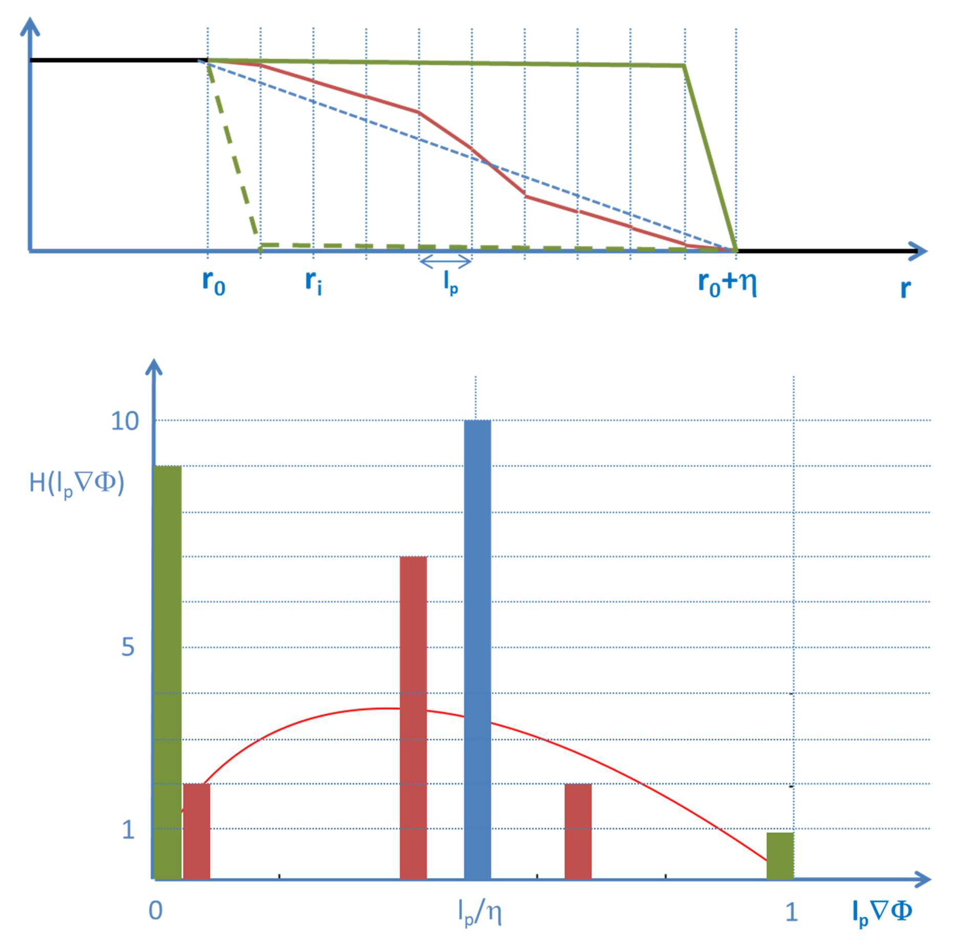
Figure 8.
Upper left: Incomplete list of models for a statistical/entropic description of entities in physics and in information theory. Most of these models reveal a logarithmic term as a common ingredient. None of these expression comprises gradients and/or Laplacian operators. Upper right: Incomplete list of models for a spatio-temporal description of stationary solutions or for the evolution in physics systems. Many of these models have a Laplacian operator as a common ingredient. Bottom: Entropy formulations comprising gradients as depicted in the present paper provide a bridge between these two model worlds.

Publisher’s Note: MDPI stays neutral with regard to jurisdictional claims in published maps and institutional affiliations. |
© 2018 by the author. Licensee MDPI, Basel, Switzerland. This article is an open access article distributed under the terms and conditions of the Creative Commons Attribution (CC BY) license (https://creativecommons.org/licenses/by/4.0/).
Share and Cite
MDPI and ACS Style
Schmitz, G.J. Entropy and Geometric Objects. Proceedings 2018, 2, 153. https://doi.org/10.3390/ecea-4-05007
AMA Style
Schmitz GJ. Entropy and Geometric Objects. Proceedings. 2018; 2(4):153. https://doi.org/10.3390/ecea-4-05007
Chicago/Turabian StyleSchmitz, Georg J. 2018. "Entropy and Geometric Objects" Proceedings 2, no. 4: 153. https://doi.org/10.3390/ecea-4-05007
APA StyleSchmitz, G. J. (2018). Entropy and Geometric Objects. Proceedings, 2(4), 153. https://doi.org/10.3390/ecea-4-05007