Proceeding Paper

Sustainable Development: Evaluating Optimal Technique for Spatial Data Forecast †

Civil Engineering Department, BITS, Pilani 333031, India
*
Author to whom correspondence should be addressed.
Presented at the Economy, Sustainable Development and Energy International Conference (ESDEIC), Edinburgh, Scotland, UK, 25–27 June 2018.
Proceedings 2018, 2(22), 1371; https://doi.org/10.3390/proceedings2221371
Published: 30 October 2018

Abstract

:
This paper is an approach to forecast the spatial data in time series domain. Normally in GIS (Geographical Information System), we need raster forecasting. Moving average, exponential smoothing, and linear regression methods of forecasting are used over one-dimensional data. Present work concentrates on using these methods on satellite images applying them from pixel to pixel of historical temporal satellite data. An example set of satellite images from years 2011 to 2015 has been used to forecast the image in the year 2016. GIS tools have been developed in ArcGIS 10.1 using python to implement the methods of forecasting. Forecasted and actual images of the year 2016 have been compared by calculating the Normalized Difference Vegetation Indices (NDVI) and change detection to identify the best method.

1. Introduction

GIS has been used for the purpose of presentation and analysis of the spatial data worldwide providing an effective platform for gathering different types of information from various sources into one system [1]. It represents a useful solution to the management of vast naturally spatially variable datasets [2]. Forecasting should not only visualize the data in GIS but also estimate its evolution [3]. Scenario development is a method of identifying the different possible circumstances for a certain resource of consideration with respect to several factors affecting it. One among all such scenarios is business as usual (BAU) which follows the same trend as of its historical data. Various methods of forecasting have been used for evaluating the business as usual (BAU) scenarios. Certain methods encountered are exponential smoothing, moving averages and regressions [4]. This paper is an attempt to forecast variables with the three mentioned methods of forecasting over a historical dataset of five raster images.

1.1. Moving Average Method

Moving average method of forecasting is one of the time series technique which uses only recent history and represents multiple observations. It places more weight on the most recent observation [5,6]. The steps performed in the method are shown as:
  • Calculate Simple Moving Average (SMA) with N = 2, 3, 4 and 5.
M ( t ) = X ( t ) +   X ( t 1 ) + + X ( t N + 1 ) N
2.
Calculate Double Moving Average (DMA) with N = 2, 3, 4 and 5.
  M 2 ( t ) = M ( t ) + M ( t 1 ) + + M ( t N + 1 ) N
3.
Forecast using the relation as:
Y ( t + T ) = a ( t ) + b ( t ) T
where; a ( t ) = 2 M ( t ) M 2 ( t ) and b ( t ) = 2 ( M ( t ) M 2 ( t ) ) N 1
Note: M(t) and M2(t) are SMA and DMA respectively. X ( t ) + X ( t 1 ) + + X ( t N + 1 ) is the sum of values of historical data from t … t − N + 1.
In order to consider average for the maximum number of historical data, we have taken N = 3.

1.2. Exponential Smoothing Method

In exponential smoothing forecast is just a weighted sum of the last observation and the previous forecast i.e., it gives more weight to last observation and decreasing weights to earlier observations [5,6]. The steps performed in the method are shown as:
  • Calculate Simple Exponential Smoothing estimates for different values (0.4…0.8) of α.
  S t = α X t 1 + ( 1 α ) S t 1
2.
Calculate Double Exponential Smoothing estimates for all values of α.
  S t 2 = α S t 1 + ( 1 α ) S t 1 2
3.
Forecast using the relation as:
Y ( t + T ) = a ( t ) + b ( t ) T
where; a ( t ) = 2 S t S t 2 and b ( t ) = α 1 α ( S t S t 2 )
Note: St and S2t are Simple Exponential smoothing and Double Exponential Smoothing respectively. Xt−1 is previous to forecasting term and α is called the smoothing factor.
In order to consider our quantity of historical data, we have taken α = 0.45 since α = 1 d , where d = number of data [4].

1.3. Linear Regression Method

This is a causal model, where an attempt is made to setup a mathematical relationship between the variable of interest and causal factors, and forecast by inserting the values of the causal factors into the mathematical model [5,6]. For n historical data points ( x 1 ,     y 1 ), ( x 2 ,     y 2 ), …, ( x n ,     y n ), forecasted value of y i for the desired xi can be obtained by the relation defined as:
y i = a + b x i
where a = y ¯ − b x ¯ ; y ¯ = i = 1 n y i n ; x ¯ = i = 1 n x i n and b = i = 1 n x i y i   x ¯   i = 1 n y i i = 1 n x i 2   x ¯   i = 1 n x i

2. Methodology

Satellite data for various consecutive historical time steps (years/months/days) depending upon their availability is collected. Such data has certain intensity value at every coordinate or pixel (x, y, z) where x, y, and z denote the band, row, and column respectively for any satellite data. All the historical intensity values corresponding to a pixel are used to forecast its intensity for the future time step. Three methods of forecasting i.e., moving average (MA), exponential smoothing (ES), and linear regression (LR) are applied one by one on the historical dataset to determine the forecasted satellite data. Later NDVI images for each forecasted data and original data are generated. Generated NDVI images are classified into two classes covering vegetation and non vegetation parts respectively. Change detection is applied to the original NDVI image and forecasted NDVI images to identify the best method among three selected for forecasting the spatial data.

3. Implementation

The methodology has been implemented over a region comprising of nine villages in Chirawa region of district Jhunjhunu in the Rajasthan state of India. The region falling under the study area has been clipped from temporal Resourcesat 2 LISS 4 satellite images with spatial resolution of 5 m, for years 2011 to 2016 procured from NRSA (National Remote Sensing Agency), India. Images from years 2011 to 2015 have been used for implementing the methodology while the image for the year 2016 is used for validation. Python tools have been developed to forecast as per the three methods. The time step required in the tools is given as 1,1, and 6 for MA, ES, and LR respectively to forecast satellite image for the year 2016.

4. Results and Discussion

The actual and forecasted images for the year 2016, classified into vegetation and non vegetation parts as per generated NDVI [7] are shown in Figure 1a–d. Classification and change detection statistics are presented in Table 1 and Table 2. Among all the three methods of forecasting applied to the satellite images over a selected region, exponential smoothing method presents better results in comparison to moving average and linear regression methods. It reflects about 78.5% match of vegetation class to the original image with about 36.5% change of pixels which is far better than other two methods.

5. Conclusion

GIS tools developed for forecasting spatial data using various extrapolation methods can help in generating various possible outcomes in the future. Such tools can be used in scenario planning activities for the data having geographical relevance. Among all the three selected methods of forecasting, exponential smoothing has given the best results over the data set chosen. These statistics would vary depending upon the quantity of historical data. Very high significance and variance of vegetation in the images as compared to a negligible variance of other features required the generation of NDVI images and change detection for validation purpose. This may work for predicting the other natural features as well, except men-made or artificial features. This process will help to forecast the z-values only instead of predicting the spread of features. It will be suitable for raster data such as interpolated rainfall maps, interpolated temperature maps, etc. for various historical years.

References

  1. Jaedicke, C.; Syre, E.; Sverdrup-Thygeson, K. GIS-aided avalanche warning in Norway. Comput. Geosci. 2014, 66, 31–39. [Google Scholar] [CrossRef]
  2. Feidas, H.; Kontos, T.; Soulakellis, N.; Lagouvardos, K. A GIS tool for the evaluation of the precipitation forecasts of a numerical weather prediction model using satellite data. Comput. Geosci. 2007, 33, 989–1007. [Google Scholar] [CrossRef]
  3. Castrillón, M.; Jorge, P.A.; López, I.J.; Macías, A.; Martín, D.; Nebot, R.J.; Sabbagh, I.; Quintana, F.M.; Sánchez, J.; Sánchez, A.J.; et al. Forecasting and visualization of wildfires in a 3D geographical information system. Comput. Geosci. 2011, 37, 390–396. [Google Scholar] [CrossRef]
  4. Armstrong, J.S. Long-Range Forecasting from Crystal Ball to Computer, 2nd ed.; John Wiley & Sons: Hoboken, NJ, USA, 1985; pp. 160–172. [Google Scholar]
  5. Makridakis, S.; Wheelwright, S.C.; Hyndman, R.J. Forecasting Methods and Applications, 3rd ed.; John Wiley & Sons: Hoboken, NJ, USA, 2008; pp. 81–231. [Google Scholar]
  6. Gupta, R. Introduction to Systems. New Age International, 2005; pp. 468–475. [Google Scholar]
  7. Lillesand, T.; Kiefer, R.W.; Chipman, J. Remote Sensing and Image Interpretation, 6th ed.; John Wiley & Sons: Hoboken, NJ, USA, 2014; p. 464. [Google Scholar]
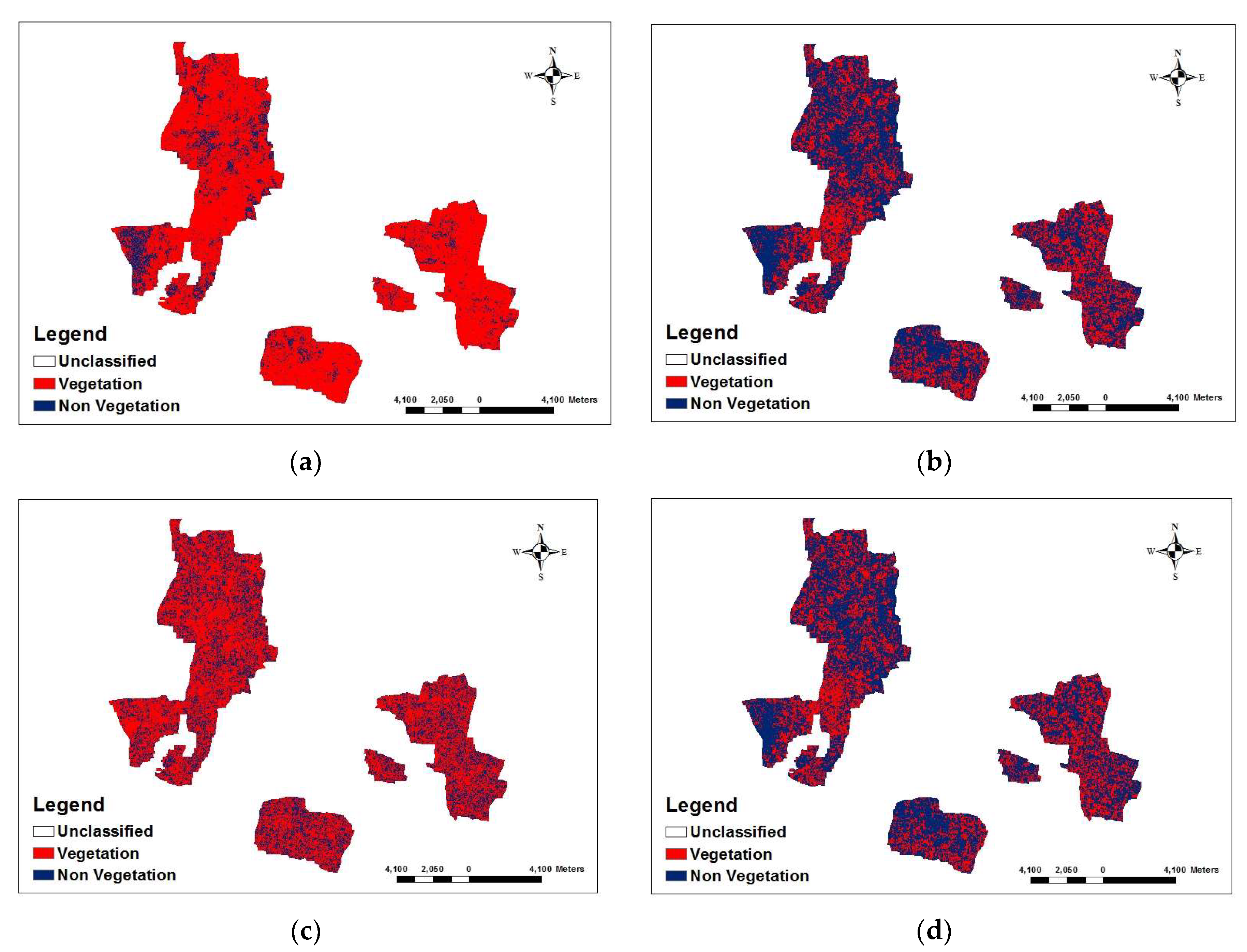
Figure 1. Vegetation based classified images for the year 2016: (a) Actual image; (b) Moving average forecasted image; (c) Exponential smoothing forecasted image; (d) Linear regression forecasted image.
Proceedings 02 01371 g001
Table 1. Vegetation match in percentage of actual image with forecasted images of the year 2016.
Classified Images of 2016VegetationNon VegetationVegetation Match (%)
Actual3,686,444660,042100
MA1,666,6942,688,77045.2114287
ES2,894,6811,460,52978.5223104
LR1,669,7822,685,67445.295195
Table 2. Change detection in percentage of actual image with forecasted images of the year 2016.
Change inIncrease by 10%Decrease by 10%Total ChangeChange in Pixels (%)
Actual & MA2,118,07987,3082,205,38750.73953994
Actual & ES1,196,802391,6041,588,40636.54460178
Actual & LR2,125,08297,9872,223,06951.14635133
Publisher’s Note: MDPI stays neutral with regard to jurisdictional claims in published maps and institutional affiliations.

