Abstract
Data driven approaches for human activity recognition learn from pre-existent large-scale datasets to generate a classification algorithm that can recognize target activities. Typically, several activities are represented within such datasets, characterized by multiple features that are computed from sensor devices. Often, some features are found to be more relevant to particular activities, which can lead to the classification algorithm providing less accuracy in detecting the activity where such features are not so relevant. This work presents an experimentation for human activity recognition with features derived from the acceleration data of a wearable device. Specifically, this work analyzes which features are most relevant for each activity and furthermore investigates which classifier provides the best accuracy with those features. The results obtained indicate that the best classifier is the k-nearest neighbor and furthermore, confirms that there do exist redundant features that generally introduce noise into the classification, leading to decreased accuracy.
1. Introduction
Human activity recognition (HAR) is a key component to a broad range of application areas including ambient assisted living, connected health and pervasive computing. It is commonly used in monitoring the activities of elderly residents to support management and prevention of chronic disease. Another common application area of HAR is within smart homes. It is used in this scenario to monitor the health and wellbeing of inhabitants by tracking their daily activities [1]. HAR can be generally classified as belonging to two categories: sensor-based or vision-based. Most notably, sensor-based activity recognition has attracted considerable research interest in pervasive computing due to advancements with sensor technologies and wireless sensor networks [2]. A frequently utilized wearable sensor for monitoring human activities is the accelerometer, which is particularly effective in observing movements such as walking, running, standing, sitting, and ascending stairs [3].
Feature selection methods [4] provide a means of selecting a subset of relevant features to use with a classifier from a dataset. Thus, these methods aim to identify which features are relevant and can indicate if there are interdependency relationships between them. The use of feature selection methods has been conducted within smart homes utilizing sensor technologies and wireless sensor networks [5,6,7] as well as with wearable devices [8,9]. In these studies, feature selection methods were applied to the entire dataset containing multiple activities, identifying the most relevant features that generalize across all target activities. In some datasets, certain features may be relevant for a subset of similar activities (scenario) in the dataset and not for another scenario in the same dataset. This fact can lead to the classification algorithm providing less accuracy in the scenario where the feature is not relevant.
This contribution analyzes, per scenario in a dataset, which features are the most relevant and which classifier works best with those features. This study is crucial to provide researchers with a guide of the most relevant features per activity type, and the classification algorithm that provides the best accuracy for that scenario (kind of similar activities) and those features. To do so, an experimentation for HAR using a recently collected dataset [10] is carried out. This dataset contains features derived from acceleration data collected from a wearable device. In this experimentation, the evaluated dataset contains six different scenarios: self-care, exercise (cardio), house cleaning, exercise (weights), sport and, finally, food preparation, representing 18 activities in which two popular feature selection methods, in conjunction with five well known classification algorithms, are evaluated.
The remainder of the paper is structured as follows: Section 3 reviews the dataset evaluated in the experimentation as well as the two feature selection methods and the five classification algorithms that will be analyzed in this contribution. Section 4 presents the proposed method to carry out the experimentation, which is divided in three groups. Section 5 presents the obtained results in the experimentation. Section 6 discusses the obtained results in order to identify the more relevant features per scenario and the most accurate classifier in the evaluated dataset. Section 6 presents the conclusions and future works.
2. Materials
In this section, the evaluated dataset used in the experimentation is reviewed, paying special attention to the features that are computed from the sensor acceleration data. Furthermore, a review of feature selection methods is provided accompanied by a brief review of the five well-known classification algorithms that will be evaluated in the experimentation.
2.1. Dataset
The dataset was collected by 141 undergraduate students at Ulster University in a controlled environment, following a data collection protocol. Students collected triaxial accelerometer data from a wearable accelerometer (Shimmer 2R, Shimmer Sensing, Dublin Ireland, Republic of Ireland) whilst carrying out 3 of the 18 investigated activities across 6 scenarios of daily living. Data was collected at a sample rate of 51.2 Hz. Data was processed using each axis of the accelerometer independently (x, y and z). Furthermore, the three axis were combined to extract the signal magnitude vector (SMV), Equation (1). The SMV is independent of orientation of the sensor node and is therefore a crucial step, particularly as the sensor was permitted to be placed on either the right or left wrist during the data recordings.
The accelerometer signals, including the SMV, were partitioned into 4 s (204 samples) non-overlapping windows. Table 1 presents the number of instances generated per windowed class. In total, 9612 instances were approximately equally represented across the 18 investigated activities, which are grouped into 6 scenarios.

Table 1.
Activities grouped by scenarios with their ids and the No. of instances.
The set of common features, defined in previous work [8,9] were extracted from the x, y, z axis and SMV, as is presented in Table 2. These features were selected to represent both temporal and frequency domain information. Features 1–24 are common statistical metrics, computed from the time domain and extracted from the SMV. Feature 25 (Signal Magnitude Area (SMA)) has been found to be a suitable measure for distinguishing between static and dynamic activities when employing triaxial accelerometer signals [9]. It is calculated by applying Equation (2).
where , , represent the acceleration signal along the x-axis, y-axis, and z-axis, respectively.
Table 2.
Initial considered feature.
Feature 26 (Spectral Entropy) is the sum of the squared magnitude of the discrete fast Fourier transform (FFT) components of a signal. Feature 27 (Total Energy), is the sum of the squared discrete FFT component magnitudes of the SMV. The sum is divided by the window length for the purposes of normalization Equation (3). This feature has been reported to result in accurate detection of specific postures and activities [11]. For instance, the energy of a subject’s acceleration can discriminate low intensity activities such as lying from moderate intensity activities such as walking or high intensity activities such as jogging. If ×1, ×2, ... are the FFT components of the window, then the energy can be represented by Equation (3):
where SMVi are the FFT components of the window for the SMV axis and |w| is the length of the window.
2.2. Feature Selection Methods
Feature selection methods are carried out in order to reduce the size of the dataset, keeping as much information as possible about the domain without causing a negative impact on the classification accuracy [4]. Therefore, irrelevant and redundant features are eliminated. Reducing the number of these features clearly improves the time taken to deploy a learning algorithm and assists in obtaining a better insight into the concept of the underlying classification problem [4].
Feature selection attempts to select the minimal sized subset of features according to the following criteria: (i) the classification accuracy does not significantly decrease; and (ii) the resulting class distribution, given only the values for the selected features, is as close as possible to the original class distribution, given all features.
Figure 1 illustrates the process of feature selection methods that consists of the following three steps in an iterative process. First, the generation procedure attempts to discover optimal feature subsets that summarize the whole feature set, reducing the computational complexity. In the case of a dataset that contains N features, the total number of candidate subsets to be generated is 2N. Second, an evaluation function measures the discriminating ability of a feature, or subset of features, in order to distinguish the different class labels. Finally, it is necessary to establish a criterion that indicates when the process is finished. The choice of stopping criterion may depend on the generation procedure and the evaluation function. This criterion can be a maximum iteration number or when a condition is achieved, for example, a number of iterations.
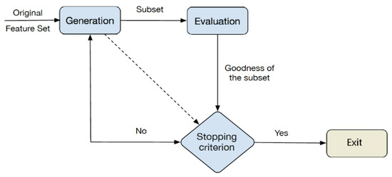
Figure 1.
Scheme of a feature selection method.
In this contribution, two feature selection methods have been used; one of them is based on a consistency measure while the other is based on a dependence measure.
On the one hand, a feature selection method based on a consistency measure so called consistencySubsetEval [12] is applied. This method evaluates the worth of a subset of features by the level of consistency in the activity class when the training instances are projected on the subset of features. So, subsets of features are highly correlated with the activity class, considering a low intercorrelation. In the evaluation functions based on the consistency measure case, the consistency of any subset can never be lower than that of the full set of features.
On the other hand, a feature selection method based on a dependence measure, CfsSubsetEval [13] is applied. This function evaluates the worth of a subset of features by considering the individual predictive ability of each feature with the redundancy degree between them. So, the subsets of features that are highly correlated with the activity class are preferred, taking into account a low intercorrelation.
2.3. Classification Algoritms
The classification algorithms, which will be evaluated in the experimentation of this work are regarded among the most popular algorithms employed for data driven approaches [3]. In this kind of approach, activity models learn from pre-existent large-scale datasets of users’ behaviors using data mining and machine learning techniques. In this contribution, the following classification algorithms have been used:
- -
- Naive Bayes classifier (NB) [14]. The basic idea in NB classifier is to use the joint probabilities of sensors and activities to estimate the category probabilities given a new activity. This method is based on the assumption of sensor independence, i.e., the conditional probability of a sensor given an activity is assumed to be independent of the conditional probabilities of other sensors given that activity.
- -
- Nearest Neighbour (KNN) [15]. This classifier is based on the concept of similarity [7] and the fact that similar patterns have the same class label. An unlabeled sample is classified with the activity label corresponding to the most frequent label among the k nearest training samples.
- -
- Decision Table (DT) [16]. This classifier is based on a table of rules and classes. Given an unlabeled sample, this classifier searches for the exact match in the table and returns the majority class label among all matching samples, or informs no matching is found.
- -
- A Multi-Layer Perceptron (MLP) [17] is a feedforward neural network with one or more layers between input and output layer. Each neuron in each layer is connected to every neuron in the adjacent layers. The training data is presented to the input layer and processed by the hidden and output layers.
- -
- Support Vector Machines (SVMs) [18]. This method focuses on a non-linear mapping to transform the original training data into a higher dimension. Within this new dimension, it searches for the linear optimal separating hyperplane. A hyperplane is a decision boundary that separates the tuples of one activity from another.
3. Method
This section presents the proposed method to analyze the evaluated dataset per scenario, to ascertain which features are the most relevant and to determine which classifier works best with those features. The method is divided into the following three groups:
- -
- The first experiment (Exp1) evaluates the complete dataset with the 27 features in order to establish the accuracy with each classification algorithm, considering the 6 scenarios.
- -
- The second experiment (Exp2) evaluates two feature selection methods in the complete dataset. The experiment Exp2.A applies the consistencySubsetEval method per each classification algorithm and the experiment Exp2.B applies the CfsSubsetEval method per each classification algorithm.
- -
- The third experiment (Exp3) transforms the complete dataset into six different datasets per scenarios. Therefore, per each scenario, the classes of that scenario are preserved and the rest of the classes are considered as negative. For each scenario, from scenario 1 (S1) to scenario 6 (S6), two experiments are carried out according to the two feature selection methods: ‘A’ for the consistencySubsetEval method and ‘B’ for the CfsSubsetEval method. For example, Exp3.S1A is the experiment with the adapted dataset for Scenario 1 when the consistencySubsetEval method is applied. Another example, Exp3.S6B is the experiment with the adapted dataset for Scenario 6 when the CfsSubsetEval method is applied. Figure 2 illustrates the transformation process for the original dataset for the Scenario 1 in the third experiment.
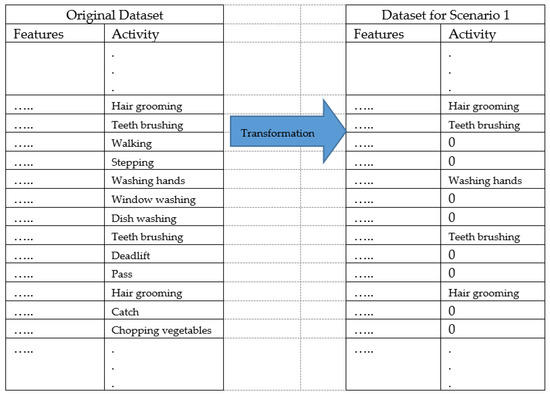 Figure 2. Transformation of the original dataset for the dataset of Scenario 1.
4. Results
The experiments have been implemented using the Weka software [18]. Weka is a Java software tool with machine learning algorithms for solving real-world data mining problems, which has GNU General Public License, GPLv3. For both feature selection methods and all classification algorithms, the default parameters of Weka have been used.
Table 3 illustrated the features considered in the three groups of experiments. Experiment Exp1 was conducted without applying a feature selection method. In Exp2A and Exp2B, the consistencySubsetEval and CfsSubsetEval methods were applied, respectively. Finally, from Exp3.S1A to Exp3.S6A, each scenario was adapted to each dataset, applying the consistencySubsetEval method, and from Exp3.S1B to Exp3.S6B, each scenario was adapted to each dataset, applying the CfsSubsetEval method. If the cell indicates a Y (Yes), that characteristic was selected by the feature selection method, otherwise, the cell indicates an N (No).
Table 3.
Features considered in each experimentation.
Table 4 presents the results from the experiment, citing the classification accuracy for each. Let be the number of samples of activities the number of samples of activities correctly classified, the classification accuracy is defined by Equation (4):
Table 4.
Classification accuracy obtained per each experimentation in each classification algorithm by using a 10-fold cross validation.
The tests were executed, employing a 10-fold Cross-Validation. The main advantage of cross-validation is that all the samples in the dataset are eventually used for training and testing and therefore avoids the problem of considering how the data is partitioned.
5. Discussion
In this Section, the computed accuracy results are analyzed, per scenario investigated, in order to identify which features were the most relevant and which classifier was found to work best with those features.
Regarding Experiment 1, the KNN algorithm was the classification algorithm that provided the highest accuracy. This experimentation did not apply a feature selection method and the training process was carried out with the original dataset, considering all 18 activities in the six scenarios. In this case, the ranking of the classifiers by accuracy was as follows: KNN > MLP > SVM > NB > DT.
Experiment 2 applied the consistencySubsetEval method in Exp2.A, which identified 14 features, and the CfsSubsetEval method in Exp2.B, which identified 19 features. The features that both feature selection methods excluded were {19,20,24,25,27}. Exp2.A and Exp2.B obtained very similar results with each classifier; however, Exp2.B required 6 fewer features than Exp2.A. The The common features of both methods were {2,3,6,7,8,9,14,15,21,23}. Therefore, we can consider these features are very important in the original dataset, to identify all the activities independent of each scenario. Exp2A is outperforming Exp2B, except when DT is used. (0.606 vs. 0.599). In both experiments, the best classifier was found to be KNN with the respective ranking of the classifiers matching those reported in Exp1: KNN > MLP > SVM > NB > DT.
Regarding Experiment 3, the increase in terms of accuracy when the dataset was adapted for each of the scenarios, merits remark. As mentioned above, the adaptation consisted of generating a dataset for each scenario where the activities within this scenario were included as positive and the rest of the activity classes of the other scenarios were considered as negatives. In the positive class, multiple activities are in each scenarios (see Figure 1). In the used dataset, each scenario has 3 activities. Full results for each experiment are presented in Table 5 and discussed below.
Table 5.
Relevant and not relevant features selected by the two feature selection methods.
From Scenario 1 (Self-Care), which included three activities, the consistencySubsetEval method was applied in Exp3.S1A, which identified 12 features, and the CfsSubsetEval method was applied in Exp3.S1B, which identified 11 features. The features that both feature selection methods excluded were {5,15,18,20,21,23,24,25,27} and, therefore, these were deemed irrelevant. The common features of both methods were {1,3,6,17,26} so, these features were considered very relevant with the three activities from scenario 1. Regarding the classifiers, accuracy results were very similar, however, again the best classifier was KNN (the results were the same in KNN and MLP in S1.A) and the order of the classifiers by accuracy was the same as in Exp 1: KNN > MLP > SVM > NB > DT.
From Scenario 2 (Exercise-Cardio), which included three activities, the consistencySubsetEval method was applied in Exp3.S2A, which identified 19 features, and the CfsSubsetEval method was applied in Exp3.S2B, which identified 17 features. The features that both feature selection methods excluded were {5,12,20,22,24,27}. The common features of both methods were {1,3,4,6,7,8,9,11,13,14,15,18,19,25,26} so we can consider these features relevant to identify the three activities from scenario 2. Regarding the classifiers, both accuracy results are very similar with the best classifier reported as KNN. The order of the classifiers by accuracy deviated slightly from earlier experiments in the Exp3.S2A (KNN > MLP > DT > SVM > NB) and Exp3.S2B with (KNN > MLP > DT > NB > SVM).
From scenario 3 (House cleaning), which included three activities, the consistencySubsetEval method was applied in Exp3.S3A, which identified 8 features, and the CfsSubsetEval method was applied in Exp3.S3B, which identified 12 features. The features that both feature selection methods excluded were {1,5,7,10,12,14,18,19,20,21,22,24,27} and, therefore, these were not relevant. The common features of both methods were {2,4,6,8,9,15}. In this case, we observed that the features selected by the consistencySubsetEval method were more relevant than the features selected by the CfsSubsetEval. Regarding the classifiers, in both cases, the best classifier was found to be the KNN.
From scenario 4 (Exercise-Weights), which included three activities, the consistencySubsetEval method was applied in Exp3.S4A, which identified only 3 features, and the CfsSubsetEval method was applied in Exp3.S4B, which identified 13 features. The features that both feature selection methods excluded were {2,7,8,9,12,13,15,16,19,22,23,26,27}. The common relevant features of both methods were {3,14}. In this case, we consider that the 3 features selected by the consistencySubsetEval method were equally relevant to the 13 features selected by the CfsSubsetEval because the accuracy results were very high (more than 0.92) and comparable to each other. Regarding the classifiers, in both cases, they all reported good performance with the best being KNN.
From scenario 5 (Sport), which included three activities, the consistencySubsetEval method was applied in Exp3.S5A, which identified only 5 features, and the CfsSubsetEval method was applied in Exp3.S5B, which identified 9 features. The features that both feature selection methods excluded were {5,9,10,12,13,16,17,18,19,20,22,23,24,26,27}. The common features of both methods were {3,14}. It is noteworthy that these common features were the same as those identified for scenario 4. Similar to scenario 4, we consider that the 5 features selected by the consistencySubsetEval method are more relevant than the 9 features selected by the CfsSubsetEval because, in general terms (4 of the 5 classifiers- less MLP), the accuracy results were higher in Exp3.S5A. Regarding the classifiers, in both cases, the best classifier was the KNN.
From scenario 6 (Sport), which included three activities, the consistencySubsetEval method was applied in Exp3.S6A, which identified 9 features, and the CfsSubsetEval method was applied in Exp3.S6B, which identified 12 features. The features that both feature selection methods excluded were {10,12,16,17,19,21,22,23,24,25,27}. The common features of both methods in scenario 6 were {1,6,11,13,26}. In both cases, the KNN was selected as the best classifier and the SVM was considered the worst classifier. The ranking order was KNN > MLP > DT > NB > SVM.
In general terms, the five classifiers performed better with those features selected by consistencySubsetEval. Furthermore, the most relevant features were found to be Feature 3 and Feature 6 that were selected 12 times, Feature 14 that was selected 10 times and, finally, Feature 1, Feature 4, Feature 8, Feature 11 and Feature 26 that were selected 9 times. The less relevant features were Feature 27 (Total Energy) that was never selected, Feature 24 that was selected once (in scenario 4). Feature 12, Feature 22 and Feature 20 were only selected twice: Feature 12 in Exp2A and Exp3.S1A; Feature 20 in Exp3.S4B and Exp3.S6A and; Feature 22 in Exp2B and Exp3.S1A.
Regarding the classifiers, it was clearly demonstrated that the classifier performing best, in terms of overall classification accuracy, was KNN. A perceived issue with KNN is its computational burden because the unseen sample is compared with each sample of the training dataset. For this reason, MLP and SVM are deemed good options because, in general terms, the feature selection methods improved the accuracy significantly. These classifiers (MLP and SVM) are, however, black box in nature and in the case that a classifier based on white box is necessary; DT and NB are also good options to employ alongside the investigated feature methods.
6. Conclusions and Future Works
In this contribution, an experiment for HAR has been carried out using a recently collected dataset containing 27 features derived from the acceleration data of a wearable device. The experiment analyzed 6 scenarios, each containing three activities, to distinguish which features are the most relevant and which classifier provided the highest accuracy with those features. To do so, two feature selection methods have been applied, which consider a consistency measure and a dependence measure. These are used in conjunction with five well-known classification algorithms (NB, KNN, MLP, DT, SVM). The method for this experimentation has been presented with three grouped experiments: (i) with the original dataset without applying feature selection methods, (ii) with the original dataset after applying the two feature selection methods and, finally, (iii) with the adapted dataset per scenario after applying each feature selection method. The proposal of the adapted dataset per each scenario considered the classes of that scenario and the remaining classes were considered as negative. Considering this experimentation, the most relevant and non-relevant features for scenarios have been identified.
Further work is required to investigate a greater number of features, particularly, those calculated from the frequency domain. Moreover, a broader set of feature selection methods and classification algorithms should be evaluated as well as to study the combination of two or more scenarios of the same dataset.
Supplementary Materials
The dataset used in this contribution are available online at https://drive.google.com/file/d/129wWrJI8N2Y-pUtt-B6iO8upVD4p87VD/view?usp=sharing
Author Contributions
Conceptualization, M.E., N.I., I.C. and C.N.; Methodology, M.E., J.M.Q. and A.S.; Validation, M.E.y.J.M. Data collection and pre-processing, I.C., M.D. and C.N.; Writing-Review & Editing, M.E., N.I., I.C., C.N., J.M., A.S. and M.D.
Funding
This work was supported by the REMIND project, which has received funding from the European Union’s Horizon 2020 research and innovation programme under the Marie Skłodowska-Curie grant agreement No 734355. Also, this contribution has been supported by the project PI-0203- 2016 from the Council of Health for the Andalusian Health Service, Spain.
Conflicts of Interest
The authors declare no conflict of interest.
Abbreviations
| HAR | Human Activity Recognition |
References
- Aggarwal, J.K.; Xia, L.; Ann, O.C.; Theng, L.B. Human Activity Recognition: A Review. Pattern Recognit. Lett. 2014, 48, 28–30. [Google Scholar] [CrossRef]
- Gu, T.; Wang, L.; Wu, Z.; Tao, X.; Lu, J. A Pattern Mining Approach to Sensor based Human Activity Recognition. IEEE Trans. Knowl. Data Eng. 2011, 23, 1359–1372. [Google Scholar] [CrossRef]
- Chen, L.; Hoey, J.; Nugent, C.D.; Cook, D.J.; Yu, Z.; Member, S. Sensor-based Activity Recognition. IEEE Trans. Syst. Man Cybern. 2012, 42, 790–808. [Google Scholar] [CrossRef]
- Dash, M.; Liu, H. Feature selection for classification. Intell. Data Anal. 1997, 1, 131–156. [Google Scholar] [CrossRef]
- Fang, H.; He, L.; Si, H.; Liu, P.; Xie, X. Human activity recognition based on feature selection in smart home using back-propagation algorithm. ISA Trans. 2014, 53, 1629–1638. [Google Scholar] [CrossRef] [PubMed]
- Fang, H.; Srinivasan, R.; Cook, D. Feature selections for human activity recognition in smart home environments. Int. J. Innov. Comput. Inf. Control 2012, 8, 3525–3535. [Google Scholar]
- Feuz, K.D.; Cook, D.J.; Rosasco, C.; Robertson, K.; Schmitter-Edgecombe, M. Automated detection of activity transitions for prompting. IEEE Trans. Hum.-Mach. Syst. 2014. [Google Scholar] [CrossRef] [PubMed]
- Mannini, A.; Rosenberger, M.; Haskell, W.L.; Sabatini, A.M.; Intille, S.S. Activity Recognition in Youth Using Single Accelerometer Placed at Wrist or Ankle. Med. Sci. Sports Exerc. 2017, 49, 801–812. [Google Scholar] [CrossRef] [PubMed]
- Bulling, A.; Blanke, U.; Schiele, B. A tutorial on human activity recognition using body-worn inertial sensors. ACM Comput. Surv. (CSUR) 2014, 46, 33. [Google Scholar] [CrossRef]
- Cleland, I.; Donnelly, M.; Nugent, C.; Hallberg, J.; Espinilla, M.; Garcia-Constantino, M. Collection of a Diverse, Naturalistic and Annotated Dataset for Wearable Activity Recognition. In Proceedings of the 2nd International Workshop on Annotation of useR Data for UbiquitOUs Systems, Athens, Greece, 19–23 March 2018. [Google Scholar]
- Sugimoto, A.; Hara, Y.; Findley, T.; Yoncmoto, K. A useful method for measuring daily physical activity by a three-direction monitor. Scand. J. Rehabil. Med. 1997, 29, 37–42. [Google Scholar] [PubMed]
- Liu, H.; Setiono, R. A probabilistic approach to feature selection-a filter solution. In ICML; Morgan Kaufmann, 1996; Volume 96, pp. 319–327. [Google Scholar]
- Hall, M.A. Correlation-Based Feature Subset Selection for Machine Learning. Ph.D. Thesis, University of Waikato, Hamilton, New Zealand, 1998. [Google Scholar]
- Domingos, P.; Pazzani, M. On the optimality of the simple bayesian classifier under zero-one loss. Mach. Learn. 1997, 29, 103–137. [Google Scholar] [CrossRef]
- Cover, T.; Hart, P. Nearest neighbor pattern classification. IEEE Trans. Inf. Theory 1967, 13, 21–27. [Google Scholar] [CrossRef]
- Hagan, M.T.; Menhaj, M.B. Training Feedforward Networks with the Marquardt Algorithm. IEEE Trans. Neural Netw. 1994, 5, 989–993. [Google Scholar] [CrossRef] [PubMed]
- Cortes, C.; Vapnik, V. Support vector networks. Mach. Learn. 1995, 20, 273–297. [Google Scholar] [CrossRef]
- Hall, M.; Frank, E.; Holmes, G.; Pfahringer, B.; Reutemann, P.; Witten, I.H. The weka data mining software: An update. ACM SIGKDD Explor. Newslett. 2009, 11, 10–18. [Google Scholar] [CrossRef]
Publisher’s Note: MDPI stays neutral with regard to jurisdictional claims in published maps and institutional affiliations. |
© 2018 by the authors. Licensee MDPI, Basel, Switzerland. This article is an open access article distributed under the terms and conditions of the Creative Commons Attribution (CC BY) license (https://creativecommons.org/licenses/by/4.0/).