Event-Driven Real-Time Location-Aware Activity Recognition in AAL Scenarios ^†

Abstract

The challenge of recognizing different personal activities while living in an apartment is of great interest for the AAL community. Many different approaches have been presented trying to achieve good accuracies in activity recognition, combined with different heuristics, windowing and segmentation methods. In this paper we want to revisit the basic methodology proposed by a naive Bayes implementation with emphasis on multi-type event-driven location-aware activity recognition. Our method combines multiple events generated by binary sensors fixed to everyday objects, a capacitive smart floor, the received signal strength (RSS) from BLE beacons to a smart-watch and the sensed acceleration of the actor’s wrist. Our new method does not use any segmentation phase, it interprets the received events as soon as they are measured and activity estimations are generated in real-time without any post-processing or time-reversal re-estimation. An activity prediction model is used in order to guess the more-likely next activity to occur. The evaluation results show an improved performance when adding new sensor type events to the activity engine estimator. Classification results achieve accuracies of about 68%, which is a good figure taking into account the high number of different activities to classify (24).

1. Introduction

Activity recognition (AR) is a very challenging problem that has been studied by many research groups. The different approaches found in the literature differ mainly in terms of the used sensor technology, the machine learning algorithms and the realism of the environment under test [1]. Regarding sensors, some works include the use of wearables such as smartwatches that include accelerometers or gyroscopes that allow the detection of activities that depend on the motion or orientation of the person (standing, lying on the bed, walking, etc.) [2]. More common is to use environment sensors such as infrared motion detectors (PIR) or reed switches coupled to doors or objects that must be placed on a base. With this kind of sensors is possible to detect when a person leaves or enters home, uses the dishwasher or takes a remote control [3]. Other environmental sensors have been explored using RFID tags or BLE beacons for proximity detection. The use of video cameras are also very informative but usually is not admitted by users since they can intrude their privacy.

The realism of experiments differs significantly for different AR studies [1]. Some approaches are based on a sequence of predefined activities scripted to an actor. This approach is more simple since it facilitates the labor of segmenting the sensor sequences and the mapping to activity labels. More realistic experiments include concurrent activities, interleaving or even aborted activities, that can be generated from one or several persons living together. If the experiments are performed by the actor behaving naturally without following a predefined script, the dataset is even more challenging for activity detection and also for the creation of the ground-truth.

Many different algorithmic approaches have been presented [1,2,3,4,5,6,7,8,9,10,11,12,13,14,15,16,17,18] for sensor-based activity recognition, from naive Bayes, hidden Markov classifiers, AdaBoost classifiers, Decision trees, Support vector machines or conditional random fields, all combined with different heuristics, windowing and segmentation methods. These common approaches are categorized under the term Data-driven (DDA) because are based on machine learning techniques. The main advantages of those approaches are the capability to deal with uncertainty and temporal information, but require large amount of data during the learning phase. A different sensor-based activity recognition category is termed Knowledge-Driven (KDA). In this case, a set of rules in a formal language is defined in order to incorporate apriori knowledge on the flow of activities for a given context. It is an elegant and logical approach but they are weak when dealing with uncertainty [4]. Hybrid solutions have already been proposed in the literature [19] in order to try to get the benefits from each individual approach.

In this paper we want to revisit the basic methodology proposed by a naive Bayes implementation with emphasis on multi-type event-driven location-aware activity recognition. We implement a DDA approach augmented with the knowledge captured by the logical flow and temporal occurrences of activities. We will make use of a dataset recorded at the UJAmI Lab from the University of Jaén that includes a person doing daily routines in an environment equipped with binary sensors, BLE beacons, smart-floor and where the actor’s arm acceleration is measured with a smartwatch. As a novelty, we will not use any segmentation phase, so algorithms interpret the received sensor events as soon as they are measured and activity estimations are generated in real-time without any post-processing or time-reversal re-estimation. The naive Bayes classifier is complemented with an activity prediction model that is used in order to guess the more-likely next activities to occur under a recursive Bayesian estimation approach.

Next Section 2 explains the methodology to handle sensing events in our experimentation site, Section 3 the core of the activity classification engine, and Section 4 the activity classification results.

2. Methodology: Test Site and Sensor-Event Handling

2.1. Sensors and Experimentation Site

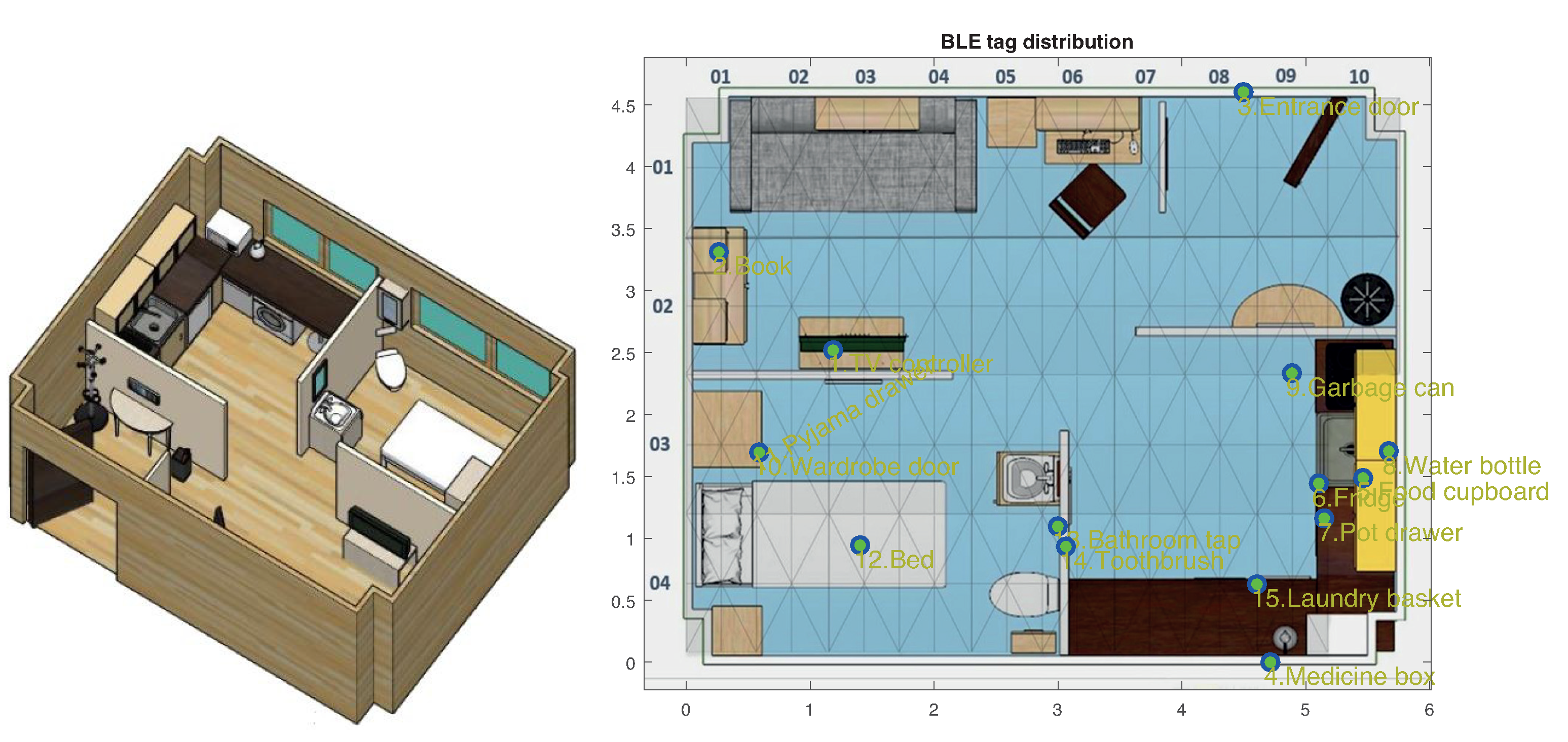
We use a dataset provided by the University of Jaén’s Ambient Intelligence (UJAmI) SmartLab (http://ceatic.ujaen.es/ujami/en/smartlab). The UJAmI SmartLab measures approximately 25 square meters, being 5.8 m long and 4.6 m wide. It is divided into five regions: hall, kitchen, workplace, living room and a bedroom with an integrated bathroom (See Figure 1).

This UJAmI site has a large variety of sensors such as a smartfloor, Bluetooth beacons, and binary (ON/OFF) sensors. Twenty floor modules are deployed covering the whole apartment surface as presented in Figure 1 (right). A total of 15 BLE beacons are also deployed as shown in that figure. A total of 31 binary switches (contact, motion and pressure; types 0, 1 and 2, respectively) are also deployed at the points listed in

Table 1. Binary sensors in the deployment (coordinates in meters).

ID	Code	Description	X	Y	Type	X*	Y*
1	M01	Door	4.5	4.6	0	4.5	4.0
2	TV0	TV	1.2	2.5	0	1.2	3.0
3	D01	Refrigerator	5.1	1.4	0	4.8	1.4
4	D02	Microwave	4.8	0.4	0	4.8	0.8
5	D03	Wardrobe clothes	0.6	1.7	0	1.0	1.7
6	SM1	Sensor Kitchen move.	5.8	2.6	1	5.8	2.6
7	SM2	Motion sensor bed	0.1	0.4	1	0.1	0.4
8	SM4	Motion sensor bedroom	1.5	0.0	1	1.5	0.0
9	SM5	Motion sensor sofa	1.6	2.5	1	1.6	2.5
10	D04	Cupboard cups	5.5	1.0	0	5.0	1.0
11	D05	Dishwasher	4.9	0.6	0	4.8	0.8
12	D07	Top WC	2.5	0.6	0	2.5	0.6
13	H01	Kettle	4.7	0.2	0	4.7	0.8
14	D08	Closet	5.5	1.9	0	4.9	2.0
15	D09	Washing machine	4.1	0.6	0	4.0	0.8
16	SM3	Motion sensor bathroom	2.7	1.3	1	2.7	1.3
17	D10	Pantry	5.5	1.5	0	4.9	1.5
18	C01	Medication box	4.7	0.0	0	4.7	0.8
19	C02	Fruit platter	4.3	0.0	0	4.3	0.8
20	C03	Cutlery	5.2	1.2	0	4.9	1.1
21	C04	Pots	5.2	1.2	0	4.9	1.1
22	C05	Water bottle	5.7	1.7	0	4.9	1.7
23	C07	Remote XBOX	1.2	2.5	0	1.2	3.0
24	C09	Tap	3.1	1.1	0	2.5	1.1
25	C10	Tank	3.1	0.4	0	2.7	0.5
26	C12	Laundry basket	4.6	0.6	0	4.6	0.8
27	C13	Wardrobe clothes	0.6	1.7	0	0.8	1.7
28	C14	Bed	1.4	0.9	2	1.4	0.9
29	C15	Kitchen faucet	5.6	1.0	0	4.9	1.0
30	S09	Pressure sofa	1.3	4.1	2	1.3	4.1
31	C08	Trash	4.9	2.3	0	4.9	2.3

with sensor location (X, Y) and potential user’s location (X${}^{*}$, Y${}^{*}$).

2.2. Real-Time Event-Driven Segmentation-Free Windowing

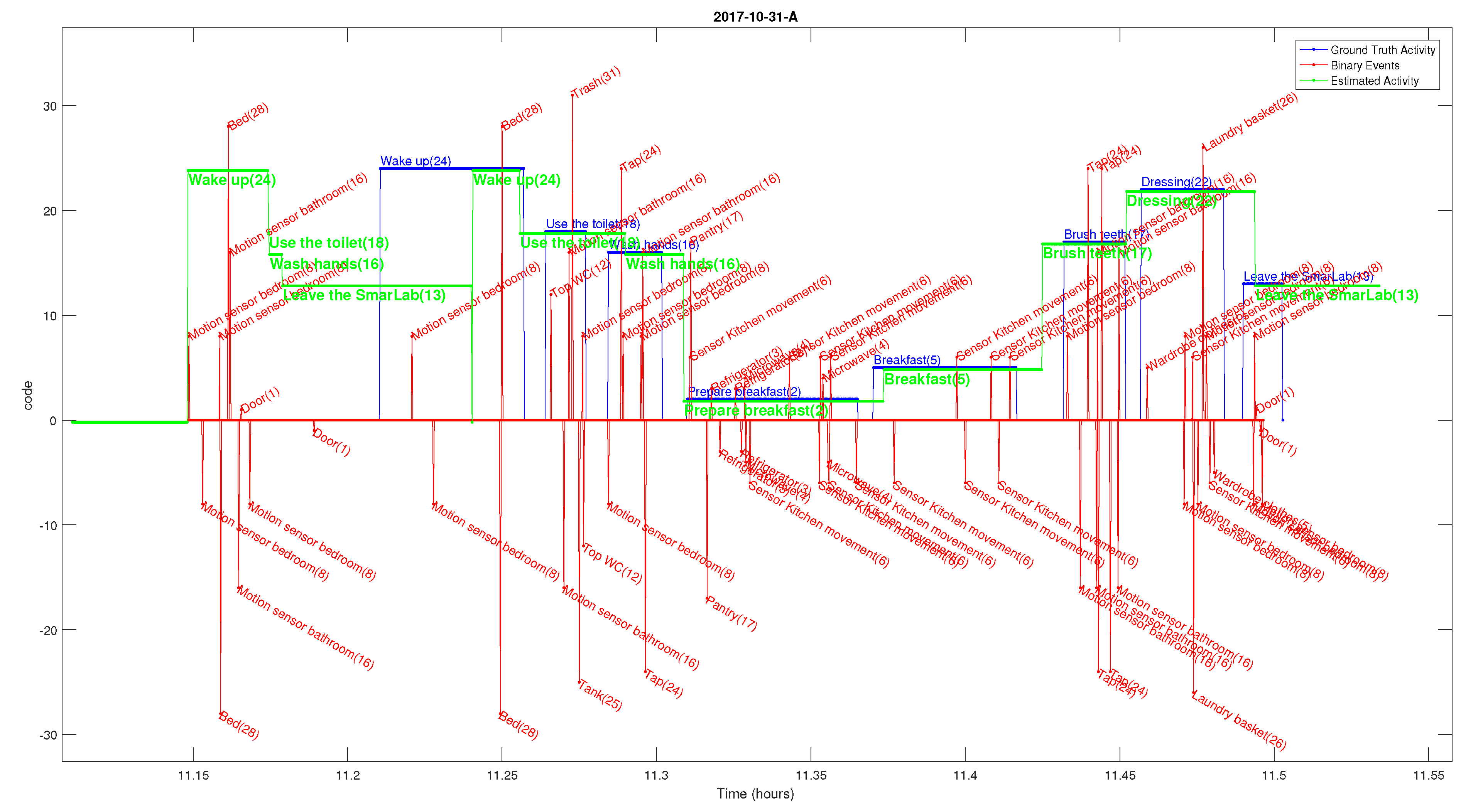
A sample of the sensor events that were registered in the morning of one of the testing days in our database is show in Figure 2. It can be seen the binary events (red spikes) which are labeled with their IDs at different heights to ease visualization. The activity ground-truth sequence (blue lines) and the estimated activities (green lines) are represented with different step-like lines with height offsets coding each of the 24 different types of activity. In a complete experimentation, additional events are generated in a similar way to the binary sensors, such as: the strongest BLE readings (those above −73 dBm), detections of floor tiles being stepped, and accelerations above a certain standard deviation. We do not show them on the same plot to avoid overlapping of information.

In the literature there are mainly three common approaches for processing streams of data like the one shown in Figure 2 [1]: (1) Explicit segmentation, (2) Time-based windowing and (3) Sensor event-based windowing. The explicit segmentation process tries to identify a window where an individual activity could be taking place, and the purpose is to separate (segment) those time intervals for a second classification stage. The second approach, the time-based windowing, divides the entire sequence of sensors events into smaller consecutive equal-size time intervals. On the other hand, the sensor event-based windowing divides the sequence into windows containing equal number of sensor events. The problem of all these approaches is defining the criteria to know how to select the optimal window values, or the number of events within a window. The result of the segmentation gives a sequence of non-overlapping intervals, so if the found intervals are too small or two large, then the classification can be confused since several activities could be present in one segment, or on the contrary, just a fraction of an activity could appear in the window.

We propose to use a new method with a fixed-size moving overlapping window to avoid doing an explicit data segmentation. We process the events as they are received, in real-time, but we do not assume that the time window contains an activity that must be classified. We assume that the window contains information that can be used to accumulate clues that increase the probability of being doing a particular activity. This segmentation-free approach is implemented using an iterative activity likelihood estimation while the fixed window is moved over time (at one-second interval displacements).

3. Activity Recognition Engine

In this section we present the core of the activity recognition estimation process, which includes the recursive Bayes approach, as well as the process and measurement models that were learnt using the sensor events in our dataset with annotated ground-truth activities.

3.1. Recursive Bayes Approach

A recursive Bayes filter is implemented as an improved version of a naive-Bayes classifier. Instead of doing a static classification based on the events present in a window, we do a dynamic process. The method uses an activity state vector $x\left(k\right)=(w_1\left(k\right),w_2\left(k\right),\dots ,w_a\left(k\right),\dots ,w_n\left(k\right))$ representing, at a given time k, the likelihood of doing a given activity a, where $a\in \{1\dots n\}$, being $n=24$ the number of different activities. The weights $w_a\left(k\right)$ of the activity state vector $x\left(k\right)$ evolve over time as new overlapped windows containing events are received or time k passes by.

The Bayes filter approach integrates a process model (probability of transition from an activity to a different one) and measurement models (probabilities of receiving an event for each activity). These models allow the classical Bayes aposteriori estimation $x^{+}\left(k\right)$ by multiplying the apriori estimate $x^{-}\left(k\right)$ based on a prediction, and the information update computed after new events are measured $x\left(k\right)$:

$$x^{+}\left(k\right)=x\left(k\right)·x^{-}\left(k\right)$$

(1)

The final activity estimation a is implemented using a decision rule (maximum a posteriori or MAP) that takes the one with the maximum probability or weight in the activity vector:

$$\mathrm{activity}\left(k\right)=\underset{a}{arg\; max}{x}^{+}\left(k\right).$$

(2)

The computation details for the apriori $x^{-}\left(k\right)$ and update $x\left(k\right)$ states are presented next.

3.2. Prediction of Activity Weights: Knowledge-Based Process Model

The training logfiles (7 days) in our dataset are analyzed in order to see the number of occurrences, the mean duration of each activity, the minimum or maximum time and its percentage of change respect to the mean value ($\Delta t$).

Table 2. Statistics from the training set of activities (7 days).

Activities		Time in Seconds			$\mathit{\Delta }\mathit{t}$(%)	Count
ID	Description	Mean	Max	Min
1	Take medication	100	158	60	98	7
2	Prepare breakfast	198	374	89	144	7
3	Prepare lunch	483	614	173	91	6
4	Prepare dinner	244	314	176	57	7
5	Breakfast	258	379	167	82	7
6	Lunch	401	649	303	86	6
7	Dinner	350	454	195	74	7
8	Eat a snack	67	95	46	74	5
9	Watch TV	420	792	123	159	6
10	Enter the SmartLab	51	73	38	68	12
11	Play a videogame	401	401	401	0	1
12	Relax on the sofa	1046	1046	1046	0	1
13	Leave the SmarLab	51	73	38	69	9
14	Visit in SmartLab	43	43	43	0	1
15	Put waste in the bin	136	247	73	128	11
16	Wash hands	57	67	36	54	6
17	Brush teeth	79	126	47	100	21
18	Use the toilet	49	70	36	69	10
19	Wash dishes	40	44	36	20	2
20	Wash clothes	54	63	45	33	6
21	Work at the table	512	637	387	49	2
22	Dressing	98	168	60	110	15
23	Go to the bed	90	128	54	82	7
24	Wake up	123	202	53	121	7
25	None	23	155	1	658	169

shows these analytic results. A total of 169 activities are detected in those 7 days. A few high frequency activities (more than 7 times in 7 days) are detected, being: Brush teeth (21 times, i.e., 3 times a day), dressing (15 times), entering/leaving the smartlab (12/9 times), put waste in bin (11) and using the toilet (10). Unfrequent activities are playing a video game (1), relax on the sofa (1), visit (1), dishwasher (2) and work on a table (2).

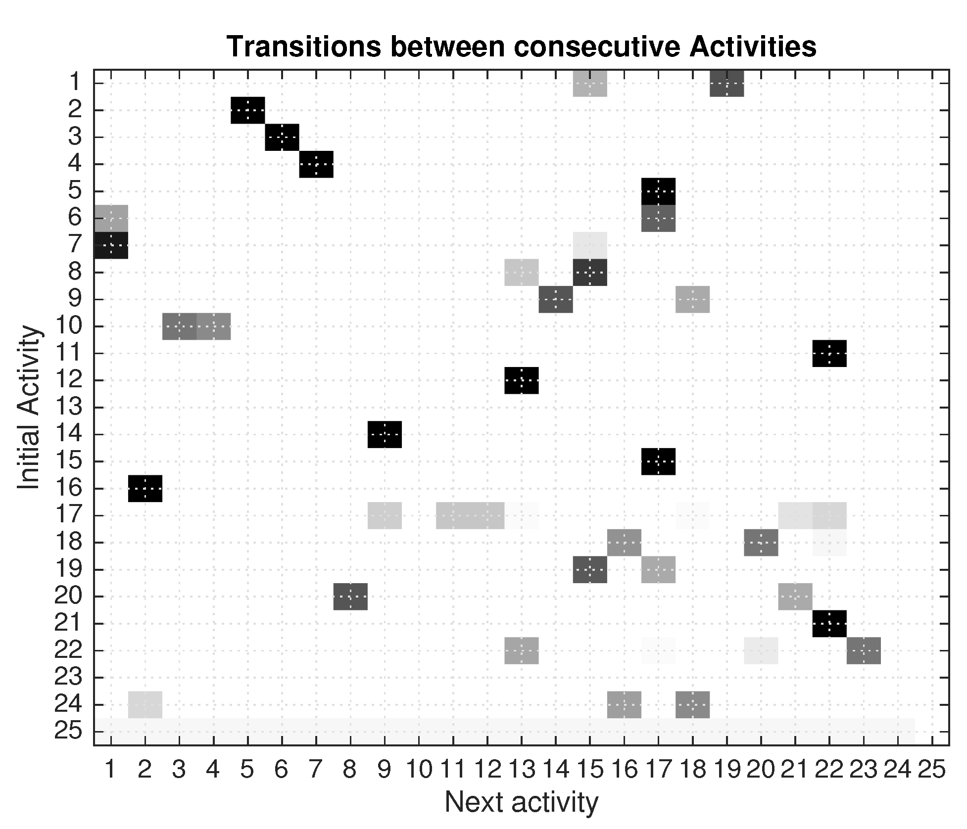
We also analyzed the correlation between one activity type and the next one, in order to identify a repetitive sequence pattern. This analysis is presented in Figure 3. It can be seen that activities numbered 2, 3 and 4 are always followed by activities 5, 6 and 7 (i.e., after Prepare breakfast the next activity is Breakfast, after Prepare lunch the next activity is Lunch, and after Prepare dinner the next activity is Dinner). We observe that after activity 7 (Dinner) is quite probable to do activity 1 (Take medication).

Many other activity transitions are correlated, and we can take advantage of this most probable activity propagation to forecast the next activity to come. We do it by predicting the new weights in the state vector $x^{-}\left(k\right)=(w_1\left(k\right),w_2\left(k\right),\dots ,w_a\left(k\right),\dots ,w_n\left(k\right))$ at a given time k, in the following way:

$$w_j\left(k\right)=w_j(k-1)+\sum _{i=1}^n\{c_i\ast w_i(k-1)\ast t(i,j)\},$$

(3)

where $t(i,j)$ is the transition correlation weight from initial activity i to the next activity j, that was learnt as a process model (Figure 3). The parameter $c_i$ is a constant that depends inversely on the average duration of initial activity i (third column in Table 2), so accelerating transitions to next activity if the previous one last few seconds, or retarding the transition if previous activity normally takes longer.

3.3. Update of Activity Weights: Sensor-Event Measurement Models

In this subsection we show the relations between the different sensor events and the performed activities. These relations will be based on the full sensors activated, in a moving window of 90 s duration, with the current activity annotated as ground-truth. Although a window could be thought as an explicit segmentation, we do not use the sensors in that window to classify and infer the activity directly, however we just accumulate clues about the potential execution of a given activity. Another implementation detail is that we do not perform sensor event fingerprinting in that window, in fact we just use one unique event of each sensor class in a given window. In that way, those events that are more active (such as PIR motion sensors) are not favored over those events that only get active once (on/off doors or contact with gadgets).

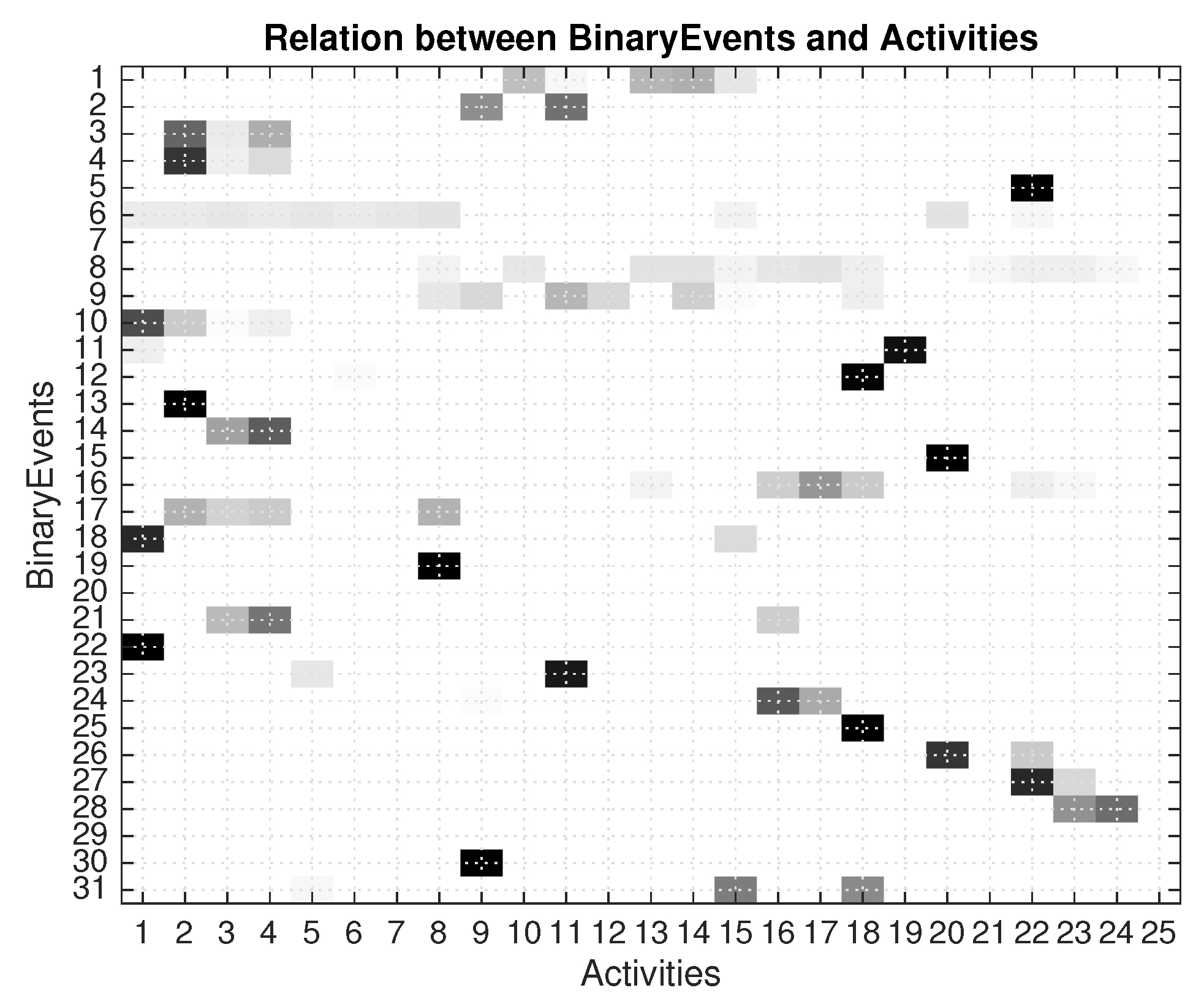
3.3.1. Binary Measurement Model

Observing the binary events for the whole training set, we obtained the probability relation matrix in Figure 4. We can observe that some sensor events clearly identify certain activities, for example, binary 5 (wardrobe clothes) is correlated with activity 22 (Dressing); or binary 19 (Fruit platter) is correlated with activity 8 (Eat a snack). On the contrary, some sensor events do not clearly define any activity, this is the case of most motion sensors (6, 7, 8, 9 , close to the kitchen, bed, bedroom and sofa, respectively).

The activity clues derived from binary sensors are accumulated in an auxiliary state vector $x_{\mathrm{binary}}$ that is computed as follows:

$$x_{\mathrm{binary}}\left(k\right)=\sum _{b=1}^{31}\delta \left(b\right)\ast \mathrm{binary}(b,:),$$

(4)

where $\delta \left(b\right)$ is dirac function if a given binary b is found in the 90-s window. And $\mathrm{binary}(b,:)$ is the binary relation vector extracted from one row out of 31 binary events in matrix in Figure 4.

3.3.2. Proximity Measurement Model

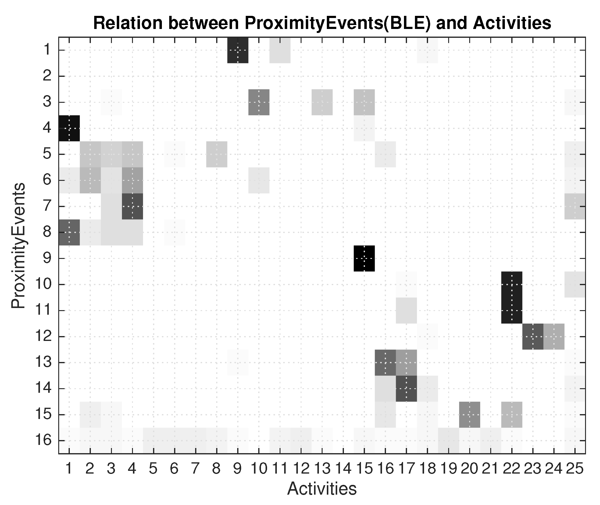
The proximity events were created from the Bluetooth Low Energy (BLE) beacons. Taking into account that BLE measurements are registered, in order to get proximity information we filter out all readings with received signal strength larger than −73 dBm. So we used only the stronger signals, that are associated with a short distance to the beacon. This information we believe can be complementary to the binary sensors, and also be discriminant of the activity under execution. The learning with the seven days training set is presented in Figure 5.

In Figure 5 we can observe that some helpful information is present. For example proximity event number 4 (Medicine box) is related to activity 1 (take medication); proximity event number 9 (garbage can) is related to activity 15 (Put waste in the bin); proximity event number 1 (TV controller) is related to activity 9 (Watch TV). On the contrary other proximity events (5 or 6), which correspond to proximities Food cupboard and Fridge, are not so clearly related to activities, but somehow represent the preparation of breakfast, lunch or dinner (activities 2, 3 and 4).

Additionally, we created a virtual proximity event (coded 16 in last row of matrix in Figure 5) that is generated when no real proximity events are sensed during more that 60 s. This extra information gives some additional clues of what type of activity the person could be doing if not close to any BLE beacon.

The proximity clues derived from BLE sensors are accumulated in an auxiliary state vector $x_{\mathrm{BLE}}$ that is computed as follows:

$$x_{\mathrm{BLE}}\left(k\right)=\sum _{B=1}^{16}\delta \left(B\right)\ast \mathrm{BLE}(B,:),$$

(5)

where $\delta \left(B\right)$ is dirac function if a given BLE B is found in the 90-s window. And $\mathrm{BLE}(B,:)$ is the BLE relation vector extracted from one row out of 16 BLE events in matrix in Figure 5.

3.3.3. Floor Measurement Model

We have also used the floor modules of the testing environment in order to relate activities with the physical position of the person. A total of 40 modules (distributed in 4 rows and 10 columns was distributed). Additionally another 2 modules are active that correspond to an area outside of the apartment. Every time a capacitive floor module reads a charge larger than 40 units, we interpret it as an floor event, which has an associated location (XY coordinates). When the person is still or on the bed, no floor signal is activated, we consider that it is also information, and a virtual event is generated when no floor signal is detected, meaning that the person is at rest or on the bed. So a total of 43 floor events were generated, and the relationship with the true activities is shown in the relation matrix in Figure 6.

We can see in Figure 6 that some apartment areas are correlated with a given activity. For example, floor codes 21, 22 and 23, which correspond to location (row: 3, columns: 1, 2 and 3) close to the wardrobe (see Figure 1), are sensed when the user is doing activity 22 (Dressing). The “No-floor” activity event (43) is not totally discriminant, but helps to increase the probability of being doing activities 11 and 12 (Play a video game and Relax on the sofa) where the user is supposed to be still.

The addition of this location-aware information is done in a similar way as in the previous binary and BLE-proximity cases:

$$x_{\mathrm{Floor}}\left(k\right)=\sum _{f=1}^{43}\delta \left(f\right)\ast \mathrm{Floor}(f,:),$$

(6)

where $\delta \left(f\right)$ is dirac function if a given Floor f is found in the 90-s window. And $\mathrm{Floor}(f,:)$ is the Floor relation vector extracted from one row out of 43 floor events in matrix in Figure 6. We also integrated information from the accelerometer in the smartwatch of the user. In this case we used the standard deviation of the acceleration magnitude. A similar matrix was done, in this case with only 2 events (motion or still). The information was not specially discriminant, since the person activities where not too related with the motion of the arm. However, we used it.

3.3.4. Time-Period Measurement Model

In order to take into account that some activities can only be performed at particular time intervals, we defined three time periods (morning, noon and afternoon). It is known that breakfast occurs during the morning, lunch at noon and dinner in the afternoon. We created the relation matrix as usual in above cases, in this occasion with a matrix of 3 rows (morning, noon and afternoon, coded as 1, 2 or 3 respectively) and the 24 activities. In Figure 7 we can see the learnt result.

From Figure 7 is clear that activities 2 and 5 (Prepare breakfast and breakfast) only occur in the morning; activities 3 and 6 (Prepare lunch and lunch) only occur at noon; activities 4 and 7 (Prepare dinner and dinner) only occur in the afternoon. Activity 9 (Watch TV) seem to occur only at noon. We take into account this information by:

$$x_{\mathrm{Day}}\left(k\right)=\sum _{d=1}^3\delta \left(d\right)\ast \mathrm{Day}(d,:),$$

(7)

where matrix $\mathrm{Day}(d,:)$ is previously binarized, and $\delta \left(d\right)$ (d from 1 to 3 periods) are equal to one just for the time period closer to the current hour of the day in the datastream.

3.3.5. Data Fusion: Measurement Model Integration

In order to fuse and combine all the information generated from the sensor events (Binary, BLE, Floor and Acce) we just accumulate them giving more weight to some of the event types. On the other hand the time periods clues are integrated by a direct product. So, the complete measurement model is implemented as follows:

$$x\left(k\right)=\{w1\ast x_{\mathrm{Binary}}\left(k\right)+w2\ast x_{\mathrm{BLE}}\left(k\right)+w3\ast x_{\mathrm{Floor}}\left(k\right)+w4\ast x_{\mathrm{Acce}}\left(k\right)\}\ast x_{\mathrm{Day}}\left(k\right),$$

(8)

where $w1$, $w2$, $w3$ and $w4$ are arbitrary weights that can be selected to take more into account some sensor events than others. We used to generate the results shown in next section these values: $(1,0.5,0.7,0.3)$, respectively.

The reason for adding up the clues from sensors, instead of multiplying them, as the naive principle of independent measurement suggest, is done to increase the robustness of sensor condition registration. In many situations not all sensor events are triggered, so it could lead to many activities being rejected, when in reality they could be being performed, so causing frequent degeneration of the probability vector (all vector equal to zero in all their activities). The addition of clues, in a voting manner, makes the solution more robust against sensor noise or incomplete measurement models.

On the other hand, we decided to use the time-of-day information ($x_{\mathrm{Day}}\left(k\right)$) in a strict manner when combined with the rest of clues obtained from the sensors. Instead of accumulating clues, we multiplied the rows of the corresponding time-period matrix, by the previous state activity vector. This is a way to reduce the confusion between similar activities, such as breakfast, lunch, or dinner, which generate similar binary, proximity and floor events. The only difference of these activities are the time at which they occur (or the ingredients used, but that is out of our control).

4. Activity Recognition Results

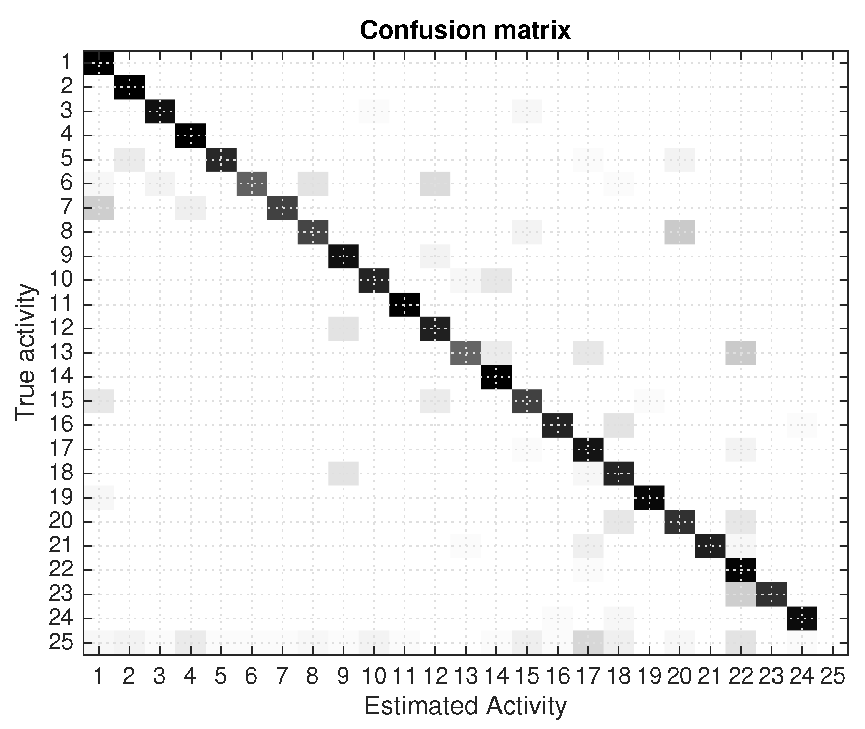
In Figure 2 we already showed one sample estimation of the activities detected for one fraction of the training tests done. We can see that the estimated activities (green step-like lines) follow up to a certain degree to the ground-truth activities (blue step-like lines). Activities are sometimes triggered incorrectly, or too soon; these results cause the generation of significant false positive, but also a majority of true positives. The overall detection results for the 7 days tests are shown in Figure 8 where a confusion matrix is presented. There is a predominant diagonal dark line, which represent the correct detections of activities, but also some off-diagonal estimations that represent estimation errors.

The best performance (using as validation test the same logfiles used for trainnig) is an 83% of true positives (in-diagonal estimates). When using different learning dataset that the days for validation, the performance goes down, as expected, to percentages between 60 and 75% (a mean of 68%), depending on the particular combinations of days used for learning and testing. These results are obtained activating all the different event sensor streams (Binary, BLE, Floor, Acce). We observed an accumulative increased performance when adding more sensor events together, being the Acce events the ones with less contribution.

Taking into account the large number of different activities (24) in the dataset, and the generality and simplified version of the algorithm, we believe that the results are not too bad. As a future work we would like to compare these results with other more sophisticated approaches in the literature (Random forest, SVM, etc.) with exactly the same dataset, in order to see the quality of the results. As an anticipated comparison, we already can find some figures, since this data set has also been used in the UCAmI Cup [20] (an off-line competition for activity recognition), so when the results get disclosed we all would see the performance using other approaches and the potential improvements generated by other algorithms. This is our algorithm’s reference method.

5. Conclusions

In this paper we have revisited the basic methodology proposed by a naive Bayes implementation with emphasis on multi-type event-driven location-aware activity recognition. Our method combined multiple events generated by binary sensors fixed to everyday objects, a capacitive smart floor, the received signal strength (RSS) from BLE beacons to a smart-watch and the sensed acceleration on the actor’s wrist. Our method did not used an explicit segmentation phase, on the contrary, it innovates interpreting the received events as soon as they are measured, and activity estimations are generated in real-time without any post-processing or time-reversal re-estimation. An activity prediction model is used in order to guess the more-likely next activity to occur, and several measurement model are added-up in order to reinforce the believe in activities. A maximum a posteriori decision rule is used to infer the most probable activity. The evaluation results show an improved performance while adding new sensor type events to the activity engine estimator. Results with a subset of the training data sets show mean accuracies of about 68%, which is a good figure taking into account the high number of different activities to classify (24 activities).