Regression Analysis and Risk Assessment of Groundwater Levels ^†

Abstract

The present research work uses Residual Kriging to estimate the groundwater level of an unconfined alluvial aquifer, as well as the trend function. The ground surface elevation is used as auxiliary variable in the trend model. Indicator Kriging is applied to detect potential vulnerable locations. Classical variogram functions are applied to determine the spatial correlation of the measurements. The risk of hydraulic head to lie below a threshold value is significant, mainly at the South and North parts of the aquifer, where the lower values of groundwater level are estimated, indicating that these areas require intense monitoring to ensure the water resources availability.

1. Introduction

An accurate estimation of hydraulic head spatial variability is indispensable to develop an effective groundwater resources management plan, especially in arid regions. Kriging [1], a method based on linear interpolation of neighboring points combined with the mean square estimate error minimization, is one of the most exact interpolation schemes. The predicted value of an unsampled location is a weighted average of the neighboring data. The weights involved in the estimator are calculated using the distance between observation and estimation points and the spatial dependence function [2,3].

Different types of Kriging have been applied to the interpolation of hydraulic head [4,5,6,7,8]. Ordinary Kriging (OK) is the most common variety of the homonymous interpolators family. The estimated values are based only on the sampled primary variable [9]. Residual Kriging (RK) combines a trend function and the interpolated -by means of OK- residuals. The regression of the principal variable is depended on auxiliary information, usually related to topographic features. The deterministic trend model of groundwater level may incorporate space polynomials [10], elevation and topographic index [2,11], rainfall data [12]. Indicator Kriging is used to estimate the probability of a variable to exceed or lie below a well-chosen threshold value at a specific point, mainly applied in risk analysis [13,14,15,16,17].

The present study applies RK to detect possible trend of the hydraulic head spatial variability of an alluvial aquifer, located at Northern Greece, considering in the estimator the ground surface elevation as secondary variable. Next, Indicator Kriging (IK) is used to predict the risk in terms of a set aquifer level limit (2.5 m above sea level), to ensure safe groundwater reserves. The two approaches provide useful information to develop an effective groundwater management strategy for the optimal manipulation of the area’s ecosystem and agriculture.

2. Study Area

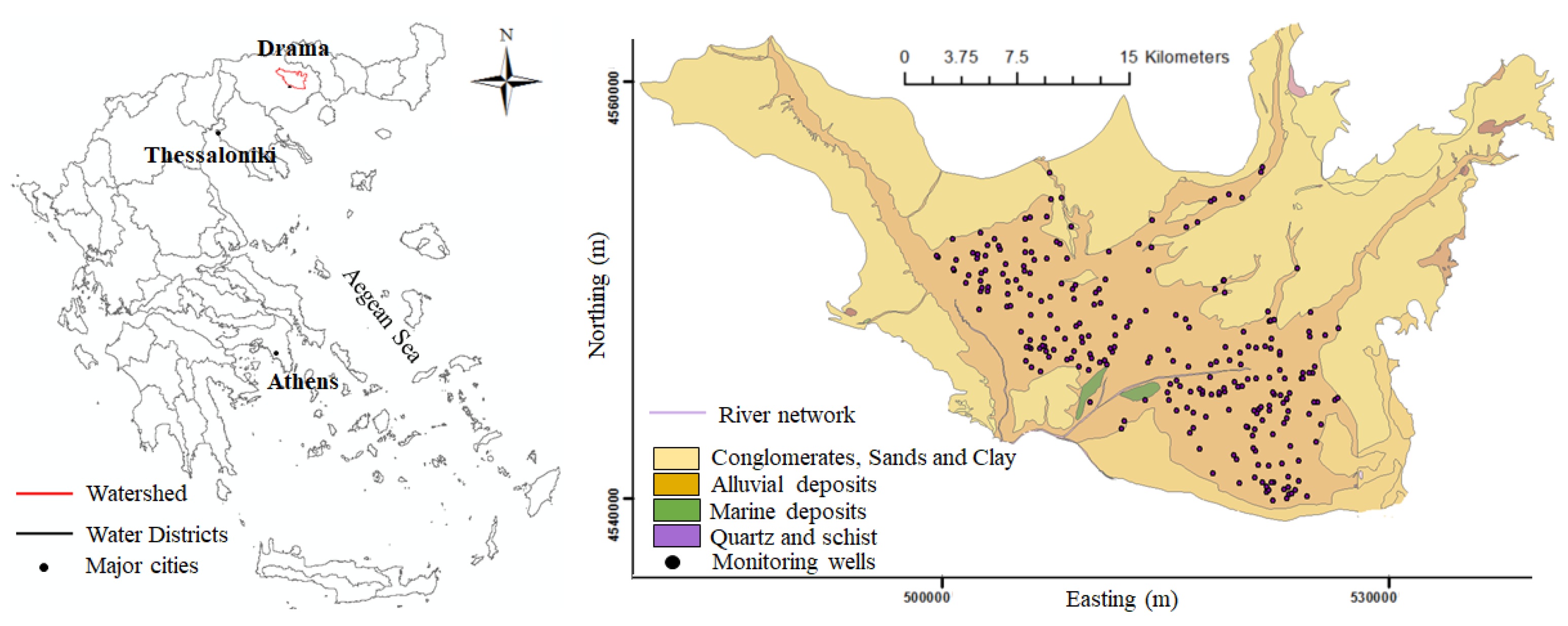
The proposed methodology is implemented in an unconfined aquifer that covers 210 km², located at the Prefecture of Drama, Greece (Figure 1). The Water District of Eastern Macedonia, where the aquifer belongs in, is characterized by both continental and Mediterranean climate and the mean annual temperature varies from 14.5 to 16.0 °C. The annual rainfall ranges between 508 mm and 576 mm.

The observed data used to develop an accurate spatial model consist of 250 hydraulic head measurements. The available values vary between 0.9 m above sea level (masl) and 22 masl. Ground surface elevation, used as auxiliary information in the trend function, varies between 48 and 137 m. Higher values of elevation are met at North-East area of the aquifer. The dataset was provided by the Water Management Authority of Eastern Macedonia and Thrace and the Environmental and Spatial Planning Authority of the Prefecture of Drama.

3. Methodology

The aim of the proposed methodology is to derive estimates, using the $z\left({\mathit{s}}_i\right)$ values (in masl) at ${\mathit{s}}_i,i=1,\dots ,N$ sampling points. An estimation point ${\mathit{s}}_0$, lying inside the convex hall of the network, moves sequentially through all the nodes of the mapping grid.

To interpolate spatially the variability of groundwater level at the study area, RK is applied. A trend model $m_Z\left(\mathit{s}\right)$ that incorporates the ground surface elevation as auxiliary information in the drift term is developed, improving in this way the accuracy of the spatial estimation [11]. The residuals are then interpolated with the help of OK.

In order to assess the risk of hydraulic head to lie below a threshold value, IK is implemented. The indicator transformed data points are obtained from a binary distribution and the conditional probability is calculated.

For each one of the two approaches, the experimental variogram is calculated and then fitted to classical theoretical models. To determine the suitable spatial model and evaluate the accuracy of the estimation, cross validation analysis is applied. The estimates are kept within the convex hull of the sampling points, as inside the quadrilateral are more accurate and precise than those outside.

3.1. Spatial Dependence

The variogram is commonly used in geostatistical analysis to express the spatial dependence of the monitoring points. The omnidirectional empirical (experimental) variogram is determined using the method of moments. The empirical variogram is fitted with isotropic classical models and the Matérn model, described in Table 1.

Table 1. Theoretical model functions: ${\sigma }_z^2$ is the variance, $\mathit{r}$ is the spatial separator vector, $\xi$ is the correlation length, $c$ is the coefficient, $H$ is the Hurst exponent, $v$ is the smoothness parameter, $\Gamma \left(·\right)$ is the Gamma function and $K_v\left(·\right)$ is the modified Bessel function of the second kind of order $v$ [18].

Model	Equation
Exponential	${\gamma }_z\left(\mathit{r}\right)={\sigma }_z^2\left[1-exp\left(-\frac{\Vert \mathit{r}\Vert }{\xi }\right)\right]$
Gaussian	${\gamma }_z\left(\mathit{r}\right)={\sigma }_z^2\left[1-exp\left(-\frac{{\Vert \mathit{r}\Vert }^2}{{\xi }^2}\right)\right]$
Spherical	${\gamma }_z\left(\mathit{r}\right)=\{\begin{array}{c}{\sigma }_z^2\left[1.5\frac{\Vert \mathit{r}\Vert }{\xi }-0.5{\left(\frac{\Vert \mathit{r}\Vert }{\xi }\right)}^3\right],0<\Vert \mathit{r}\Vert <\xi \\ {\sigma }_z^2, \Vert \mathit{r}\Vert >\xi \end{array}$
Power-law	${\gamma }_z\left(\mathit{r}\right)=c{\Vert \mathit{r}\Vert }^{2H},0<H<1$
Linear	${\gamma }_z\left(\mathit{r}\right)=c\Vert \mathit{r}\Vert$
Matérn	${\gamma }_z\left(\mathit{r}\right)={\sigma }_z^2\left\{1-\frac{2^{1-v}}{\Gamma \left(v\right)}{\left(\frac{\Vert \mathit{r}\Vert }{\xi }\right)}^v{K}_v\left(\frac{\Vert \mathit{r}\Vert }{\xi }\right)\right\}$

Table 1. Theoretical model functions: ${\sigma }_z^2$ is the variance, $\mathit{r}$ is the spatial separator vector, $\xi$ is the correlation length, $c$ is the coefficient, $H$ is the Hurst exponent, $v$ is the smoothness parameter, $\Gamma \left(·\right)$ is the Gamma function and $K_v\left(·\right)$ is the modified Bessel function of the second kind of order $v$ [18].

Model	Equation
Exponential	${\gamma }_z\left(\mathit{r}\right)={\sigma }_z^2\left[1-exp\left(-\frac{\Vert \mathit{r}\Vert }{\xi }\right)\right]$
Gaussian	${\gamma }_z\left(\mathit{r}\right)={\sigma }_z^2\left[1-exp\left(-\frac{{\Vert \mathit{r}\Vert }^2}{{\xi }^2}\right)\right]$
Spherical	${\gamma }_z\left(\mathit{r}\right)=\{\begin{array}{c}{\sigma }_z^2\left[1.5\frac{\Vert \mathit{r}\Vert }{\xi }-0.5{\left(\frac{\Vert \mathit{r}\Vert }{\xi }\right)}^3\right],0<\Vert \mathit{r}\Vert <\xi \\ {\sigma }_z^2, \Vert \mathit{r}\Vert >\xi \end{array}$
Power-law	${\gamma }_z\left(\mathit{r}\right)=c{\Vert \mathit{r}\Vert }^{2H},0<H<1$
Linear	${\gamma }_z\left(\mathit{r}\right)=c\Vert \mathit{r}\Vert$
Matérn	${\gamma }_z\left(\mathit{r}\right)={\sigma }_z^2\left\{1-\frac{2^{1-v}}{\Gamma \left(v\right)}{\left(\frac{\Vert \mathit{r}\Vert }{\xi }\right)}^v{K}_v\left(\frac{\Vert \mathit{r}\Vert }{\xi }\right)\right\}$

3.2. Residual Kriging

RK splits the random function into a smoothly varying and nonstationary trend and a random component, the residual data [9,19]. Trend subcomponents can be determined based on physical principles. Herein, the deterministic trend of the hydraulic head is estimated by finding the relationship between the topographic elevation and the hydraulic head. The estimated values are expressed as a sum of the trend function $m_Z\left({\mathit{s}}_0\right)$ and the interpolated by OK residuals ${\widehat{Z}}^{\prime }\left({\mathit{s}}_0\right)$ [20]:

$$m_Z\left({\mathit{s}}_0\right)+{\widehat{Z}}^{\prime }\left({\mathit{s}}_0\right)={\displaystyle {\sum }_{k=0}^p}{\beta }_k{q}_k\left({\mathit{s}}_0\right)+{\displaystyle {{\displaystyle \sum }}_{i=1}^{N_0}}{\lambda }_{i}z\left({\mathit{s}}_i\right), q_k\left({\mathit{s}}_0\right)=1$$

(1)

where

• ${\beta }_k$: the deterministic regression coefficients, estimated using ordinary least squares (OLS)
• $q_k\left({\mathit{s}}_0\right)$: the values of depended variables at the estimation point ${\mathit{s}}_0$
• $p$: the number of predictors
• ${\lambda }_i$: the kriging weights
• $z\left({\mathit{s}}_i\right)$: the values of the sample data
• $N_0$: the number of points included in the search neighborhood of the prediction point ${\mathit{s}}_0$.

The variance of the estimation includes the trend prediction variance ${\sigma }_d^2({\mathit{s}}_0)$ and the OK variance ${\sigma }_f^2({\mathit{s}}_0)$ of the residuals:

$${\sigma }^2({\mathit{s}}_0)={\sigma }_d^2({\mathit{s}}_0)+{\sigma }_f^2({\mathit{s}}_0)={\mathit{q}}_0^T{\left({\mathit{q}}^T{\gamma }_{Z^{\prime }}^{-1}\mathit{q}\right)}^{-1}{\mathit{q}}_0+{\displaystyle {{\displaystyle \sum }}_{i=1}^{N_0}}{\lambda }_i{\gamma }_{Z^{\prime }}\left({\mathit{s}}_i, {\mathit{s}}_0\right)+\mu$$

(2)

where

• ${\mathit{q}}_0$: the vector of $\left(p+1\right)\times 1$ predictors
• $\mathit{q}$: the matrix of $\left(N_0+1\right)\times \left(p+1\right)$ predictors at the observations in the search neighborhood
• ${\gamma }_{Z^{\prime }}$: the variogram matrix of the $\left(N_0+1\right)\times \left(p+1\right)$ residuals in the neighborhood
• $\mu$: the Lagrange coefficient [21,22].

3.3. Indicator Kriging

IK is a useful geostatistical tool that helps to estimate the probability of a variable to exceed or lie below a well-chosen threshold value at a specific point, taking at the same time into account the uncertainty of the data [13]. In the present research work, a limit that could cause problems of groundwater availability is set as a threshold value. IK estimates the probability of hydraulic head to lie below this value. The data are transformed into indicators using a binary distribution (e.g., 0 and 1). This transformation is given by the following equation:

$$I\left(z\left(\mathit{s}\right)\right)=\{\begin{array}{c}1, z\left(\mathit{s}\right)\le z^{\prime }\\ 0, otherwise\end{array}$$

(3)

where $I\left(z\left(\mathit{s}\right)\right)$ is a binary variable, $z\left(\mathit{s}\right)$ is the measured value and $z\prime$ is the cut-off (threshold) value.

The indicator variogram is estimated, using a suitable theoretical model. Kriging is applied using the usual equation to obtain predictions. The conditional probability at unsampled points based on the spatial correlation structure results in a map with values between 0 and 1, expressing the risk associated with the cutoff value [16,23]. This probability map delineates suitable and unsuitable sites regarding the examined issue, while helps that way to take decisions to prevent and/or remediate a site compared to locations with reduced or no risk [24].

4. Results

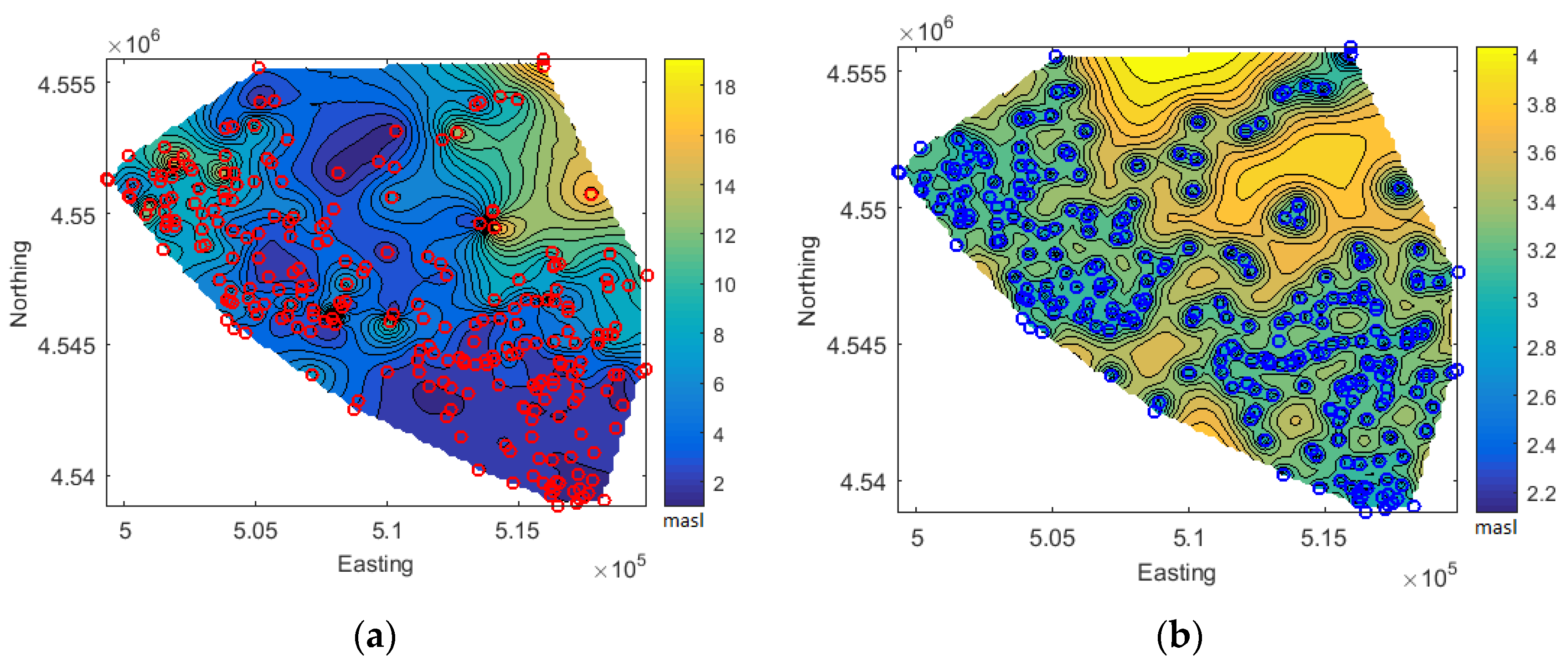
As a first step, the data are decomposed into a linear trend plus a residual value. The experimental variogram of the residuals is then calculated and fitted to the theoretical models presented in Table 1. The optimal function that adapts the experimental omnidirectional variogram is the Exponential variogram. The estimated parameters are used to determine the spatial dependence model. To estimate the distribution of the hydraulic head data at unvisited locations and the associated uncertainty, RK is applied on a 100 × 100 grid. The corresponding contour maps are shown in Figure 2.

According to Figure 2a, the groundwater level changes from South-West towards North-East, following the ground surface elevation trend. The spatial variability of the groundwater level is established with higher accuracy around the sample locations, while at the North of the aquifer significant estimation error occurs (Figure 2b).

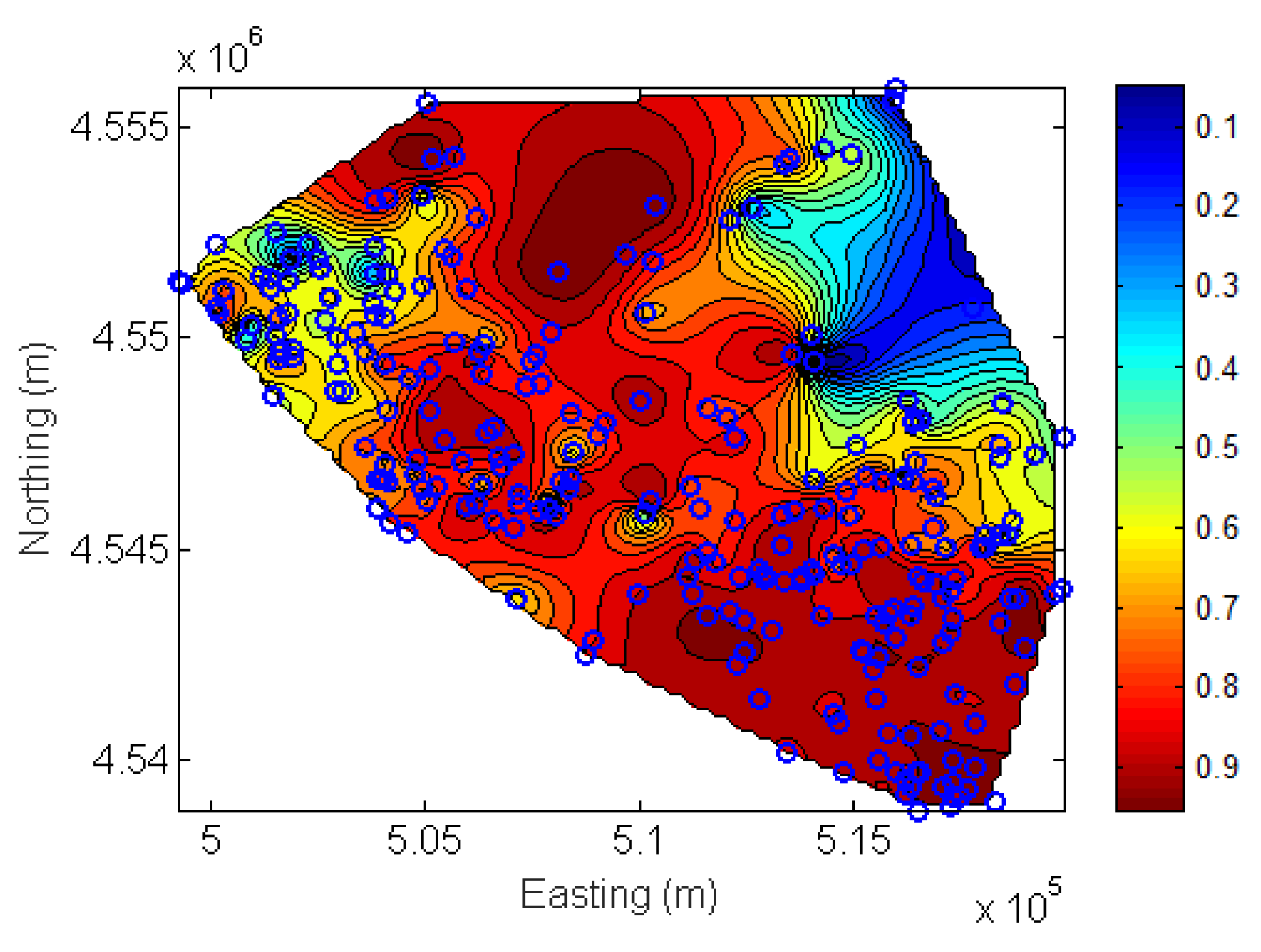
To assess the risk associated with the groundwater level spatial distribution, IK is applied. As a threshold value is set the 25th, lower, percentile of the available data values, which is equal to 2.5 masl. The indicators are interpolated applying the best-fit Power-law variogram model. The probability of the groundwater level to lie below the cut-off value is increased towards the South and the North of the aquifer, where the lower hydraulic heads are met (Figure 3).

5. Conclusions

The Exponential variogram provides the best fit to the experimental one. The ground surface elevation, an auxiliary variable with physical notion, incorporates useful information about the hydraulic head spatial distribution, interpolated by means of RK. Due to the extremely low groundwater level values predicted at specific locations, IK is applied to identify the associated risk. The method is based on the best-fit Power-law model. The risk is significant mainly at the South and North parts of the aquifer, where the lower values of groundwater level are estimated, indicating that remedial actions should take place to avoid further decline of the aquifer. As a conclusion, RK delivers a quantitative estimation that shows how the groundwater level spatial distribution is formed, when other boundary conditions are not available. On the other hand, IK provides a measure of risk that the estimates calculated for unsampled locations by RK will be below the chosen critical threshold value. Overall, the application of the two aforementioned methods, accompanied by the appropriate spatial dependence function can provide useful and reliable results in order spatial variability and potential depletion risk of the aquifer level to be identified.

References

- Krige, D.G. A statistical approach to some basic mine valuation problems on the Witwatersrand. J. Chem. Metall. Min. Soc. S. Afr. 1951, 5, 119–139. [Google Scholar]
- Desbarats, A.J.; Logan, C.E.; Hinto, M.J.; Sharpe, D.R. On the kriging of water table elevations using collateral information from a digital elevation model. J. Hydrol. 2002, 255, 25–38. [Google Scholar] [CrossRef]
- Little, L.; Edwards, D.; Porter, D. Kriging in estuaries: As the crow flies, or as the fish swims? J. Exp. Mar. Biol. Ecol. 1997, 213, 1–11. [Google Scholar] [CrossRef]
- Ahmadi, S.; Sedghamiz, A. Application and evaluation of kriging and cokriging methods on groundwater depth mapping. Environ. Monit. Assess. 2007, 129, 277–294. [Google Scholar] [CrossRef] [PubMed]
- Rivest, M.; Marcotte, D.; Pasquier, P. Hydraulic head field estimation using kriging with an external drift: A way to consider conceptual model information. J. Hydrol. 2008, 361, 349–361. [Google Scholar] [CrossRef]
- Pucci, A.A.J.; Murashige, J.A.E. Applications of universal kriging to an aquifer study in New Jersey. Groundwater 1987, 25, 672–678. [Google Scholar] [CrossRef]
- Nikroo, L.; Kompani-Zare, M.; Sepaskhah, A.; Fallah Shamsi, S. Groundwater depth and elevation interpolation by kriging methods in Mohr Basin of Fars province in Iran. Environ. Monit. Assess. 2009, 166, 387–407. [Google Scholar] [CrossRef] [PubMed]
- Delhomme, J.P. Kriging in the hydrosciences. Adv. Water Resour. 1978, 1, 225–266. [Google Scholar] [CrossRef]
- Kitanidis, P.K. Introduction to Geostatistics; Cambridge University Press: Cambridge, UK, 1997. [Google Scholar]
- Neuman, S.; Jacobson, E. Analysis of nonintrinsic spatial variability by residual kriging with application to regional groundwater levels. Math. Geol. 1984, 16, 499–521. [Google Scholar] [CrossRef]
- Varouchakis, E.A.; Hristopulos, D.T. Improvement of groundwater level prediction in sparsely gauged basins using physical laws and local geographic features as auxiliary variables. Adv. Water Resour. 2013, 52, 34–49. [Google Scholar] [CrossRef]
- Moukana, J.A.; Koike, K. Geostatistical model for correlating declining groundwater levels with changes in land cover detected from analyses of satellite images. Comput. Geosci. 2008, 34, 1527–1540. [Google Scholar] [CrossRef]
- Goovaerts, P. Geostatistics for Natural Resources Evaluation; Oxford University Press: New York, NY, USA, 1997. [Google Scholar]
- Anane, M.; Selmi, Y.; Limam, A.; Jedidi, N.; Jellali, S. Does irrigation with reclaimed water significantly pollute shallow aquifer with nitrate and salinity? An assay in a perurban area in North Tunisia. Environ. Monit. Assess. 2014, 186, 4367–4390. [Google Scholar] [CrossRef] [PubMed]
- Arslan, H. Spatial and temporal mapping of groundwater salinity using ordinary kriging and indicator kriging: The case of Bafra Plain, Turkey. Agric. Water Manag. 2012, 113, 57–63. [Google Scholar] [CrossRef]
- Chica-Olmo, M.; Luque-Espinar, J.A.; Rodriguez-Galiano, V.; Pardo-Igúzquiza, E.; Chica-Rivas, L. Categorical Indicator Kriging for assessing the risk of groundwater nitrate pollution: The case of Vega de Granada aquifer (SE Spain). Sci. Total Environ. 2014, 470–471, 229–239. [Google Scholar] [CrossRef] [PubMed]
- Liu, C.W.; Jang, C.S.; Liao, C.M. Evaluation of arsenic contamination potential using indicator kriging in the Yun-Lin aquifer (Taiwan). Sci. Total Environ. 2004, 321, 173–188. [Google Scholar] [CrossRef] [PubMed]
- Theodoridou, P.G.; Varouchakis, E.A.; Karatzas, G.P. Spatial analysis of groundwater levels using Fuzzy Logic and geostatistical tools. J. Hydrol. 2017, 555, 241–252. [Google Scholar] [CrossRef]
- Wackernagel, H. Multivariate Geostatistics: An Introduction with Applications, 3rd ed.; Springer: Berlin/Heidelberg, Germany, 2003. [Google Scholar]
- Rivoirard, J. On the structural link between variables in Kriging with external drift. Math. Geol. 2002, 34, 797–808. [Google Scholar] [CrossRef]
- Draper, N.; Smith, H. Applied Regression Analysis, 2nd ed.; Wiley: New York, NY, USA, 1981. [Google Scholar]
- Hengl, T.; Heuvelink, G.B.M.; Rossiter, D.G. About regression-kriging: From equations to case studies. Comput. Geosci. 2007, 33, 1301–1315. [Google Scholar] [CrossRef]
- Deutsch, C.V.; Journel, A.G. GSLIB. Geostatistical Software Library and User’s Guide; Oxford University Press: New York, NY, USA, 1992. [Google Scholar]
- Varouchakis, E.A.; Kolosionis, K.; Karatzas, G.P. Spatial variability estimation and risk assessment of the aquifer level at sparsely gauged basing using geostatistical methodologies. Earth Sci. Inform. 2016, 9, 437–448. [Google Scholar] [CrossRef]