A Different Angle on Quantum Uncertainty (Measure Angle) ^†

Abstract

The uncertainty associated with probing the quantum state is expressed as the effective abundance (measure) of possibilities for its collapse. New kinds of uncertainty limits entailed by the quantum description of the physical system arise in this manner.

1. Introduction

One could easily imagine the results of this presentation being reported at a physics conference long ago, well before Alice, Bob, and Charlie were part of the quantum discourse. In fact, it would have been natural for this to happen when the Copenhagen interpretation of quantum mechanics (QM) was only emerging [1]. One reason it did not occur may be that the needed association of probability and measure was not developed or appreciated at the time, although it very well could have been. Here, we obviously do not mean the use of measure theory to formalize probability [2]. Rather, what we have in mind is a generalization of measure by means of probability: the extension of measure map $\mu =\mu \left(A\right)$ onto a larger domain $\mu =\mu (A,\pi )$, where $\pi$ is a probability measure on A. The role of $\pi$ is to specify the “relevance” of various parts (measurable subsets) of A. The desired extension is then chiefly driven by two requirements. (i) $\mu (A,\pi )$ should decrease relative to $\mu \left(A\right)$ in response to $\pi$ favoring certain parts of A, so that $\pi$ involving more concentrated probability entails larger reduction (monotonicity with respect to cumulation). (ii) $\mu (A,\pi )$ should remain strictly measure-like, in that the original additivity relation involving sets A and B generalizes into one involving pairs $(A,{\pi }_A)$ and $(B,{\pi }_B)$, for all ${\pi }_A$ and ${\pi }_B$. If (i) and (ii) can be simultaneously accommodated and together with few other basic requirements, then $\mu (A,\pi )$ defines a meaningful effective measure of A with respect to $\pi$. Such a quantifier could then be used in correspondingly wider contexts, but with essentially the same meaning and significance, as that of an ordinary measure. Being a framework for assigning probabilities to events, quantum mechanics would be among prime natural settings for its use.

Whether the outlined general approach materializes into a fruitful enrichment of QM depends on the existence and multitude of the above extensions for relevant measures. In Reference [3], released during the ICNFP 2018 meeting, the extension program was completely carried out for the foundational case of the counting measure. It is the surprising results of this analysis that we point out in this presentation and that suggest, among other things, a qualitatively new outlook on quantum uncertainty [1,4]. Since the ICNFP 2018 meeting, the ensuing concept of measure uncertainty ($\mu$-uncertainty) has been fully developed in Reference [5]. Over the course of that process, effective measures were also defined for subsets of D-dimensional Euclidean space ${\mathbb{R}}^D$ with Jordan content, i.e., whose “volume” is expressible as a Riemann integral.

Since the discrete case involves somewhat specific language, we summarize the correspondence with the general case before we start. A “measurable set A” becomes simply a “collection of N objects”, and $\mu \left(A\right)$ corresponds to N. A probability measure $\pi$ is specified by probability vector $P=(p_1,p_2,\dots ,p_N)$. The construction of effective measure extension $\mu =\mu (A,\pi )$ then turns into the construction of function $\mathcal{N}=\mathcal{N}\left[P\right]$, interpreted as the effective total (effective count). The theory of these objects is referred to as effective-number theory since $\mathcal{N}$ retains certain algebraic features of integers [3]. In the same vein, functions $\mathcal{N}$ are called effective-number functions (ENFs).

In the first part of the presentation, we describe the key features and results of effective-number theory, which is a crucial stepping stone for our arguments regarding quantum uncertainty. One natural approach to constructing the theory is to view it as a tool to solve a generic counting problem of quantum mechanics, which we refer to as the quantum-identity problem [3]. In particular, consider state $\mid \psi \rangle$ and basis $\left\{\mid i\rangle \right\}\equiv \{\mid i\rangle \mid i=1,2,\dots ,N\}$ in N-dimensional Hilbert space. Is it meaningful to ask how many basis states $\mid i\rangle$ (“identities” from $\left\{\mid i\rangle \right\}$) are effectively contained in $\mid \psi \rangle$. This question can be phrased in many equivalent ways that directly relate to a particular application of interest. For example, in the context of describing localization, the inquiry would be about how many states from $\left\{\mid i\rangle \right\}$ is $\mid \psi \rangle$ effectively spread over. On the other hand, in assessing the efficiency of a variational calculation involving eigenstate $\mid \psi \rangle$ and basis $\left\{\mid i\rangle \right\}$, we would be concerned with how many $\mid i\rangle$ effectively describe $\mid \psi \rangle$. However, it is the same quantum-identity question arising in all these situations, and it entails seeking maps

$$\mid \psi \rangle ,\left\{\mid i\rangle \right\}⟶\mathcal{N}[\mid \psi \rangle ,\{\mid i\rangle \left\}\right]$$

(1)

consistently assigning the effective totals. Hence, in the context of the quantum -identity problem, the “objects” in the discrete sets are basis states $\mid i\rangle$, and their probabilistic weight is encoded in $\mid \psi \rangle$ by the quantum-mechanical rule $p_i=\mid \langle i\mid \psi \rangle {\mid }^2$. Effective-number function $\mathcal{N}$ is thus a map whose domain consists of probability vectors P so constructed. (We note here that, as part of further research, we suggest to look at many other active areas of physics to find applications for the quantum-identity problem. Given the nature of their focus, appropriately formulated questions may arise in the context of Anderson localization, quantum chaos, quantum computing/information, entanglement, thermalization, topological insulators, holography, and possibly others.) In the second part of this presentation, we argue that effective-number theory leads to a novel understanding of quantum uncertainty. In fact, the association of effective measure and uncertainty constitutes a conceptual thread connecting all of the mentioned quantum applications.

2. Effective-Number Theory

Although we are concerned with describing an abstract theory, it is useful to keep a concrete physical situation in mind when doing so. We use the elementary example of a spinless-lattice Schrödinger particle, described by wave function $\mid \psi \rangle \to (\psi \left(x_1\right),\dots ,\psi \left(x_N\right))$, for this purpose. Thus, N is the number of lattice sites and $p_i={\psi }^{★}\psi \left(x_i\right)$ refers to the probability of detecting the particle at position $x_i$. 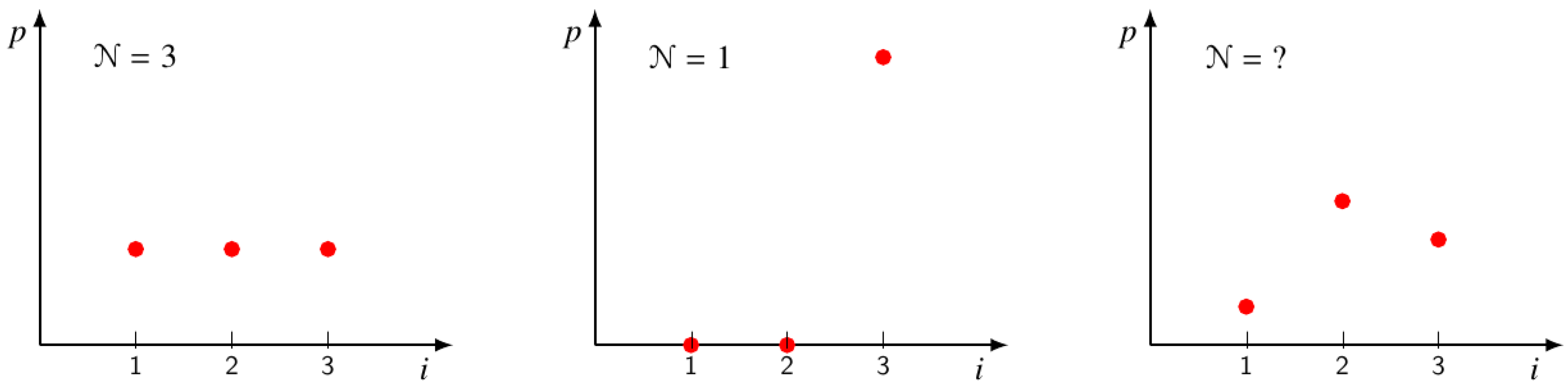In the language of quantum-identity Problem (1), we ask how many position basis states $\mid i\rangle$ is $\mid \psi \rangle$ is effectively composed of. The situation is exemplified in Figure 1, showing three probability distributions on the lattice with three sites. Clearly, all ENFs should assign $\mathcal{N}=3$ to uniform distribution (left panel) and $\mathcal{N}=1$ to $\delta$-function distribution (middle panel). The problem in question boils down to establishing whether well-founded effective numbers can be assigned to generic distributions, such as the one shown in the right panel.

Our approach to this issue was to develop an axiomatic definition of set $\mathfrak{N}$ containing all effective-number functions $\mathcal{N}$, and then analyze its properties [3]. Two of the axioms play a prominent role in shaping possible ENFs, namely, additivity and monotonicity with respect to “cumulation”. The latter is closely related to Schur concavity. Since both need some care in their formulation, we discuss them in somewhat more detail than other requirements. It should be noted that additivity, while crucial for a measure-like concept, was not part of related considerations in the past.

2.1. Additivity

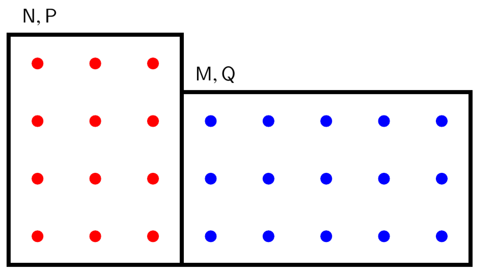
Consider the lattice Schrödinger particle on the lattice with N sites, in a state producing probability vector $P=(p_1,\dots ,p_N)$. Similarly, let the particle be restricted to a nonoverlapping lattice of M sites, generating probabilities $Q=(q_1,\dots ,q_M)$. Then, there exists a state of the particle on the combined lattice (see Figure 2) that leads to probability distribution

(2)

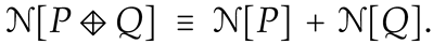
on the position basis of the combined system. Here, ⊞ denotes the concatenation operation, namely, $(a_1,\dots ,a_N)⊞(b_1,\dots ,b_M)\equiv (a_1,\dots ,a_N,b_1,\dots ,b_M)$. Note that does not change the weight ratios for position states inside the two parts of the system, thus preserving individual distribution shapes. It also properly corrects weight ratios of the position pairs from distinct parts by their respective “measures” (lattice sizes N and M). While the nominal size of the combined system is trivially given by $N+M$ (ordinary count), its effective size in a said state (effective count) has to also be additive, yielding the corresponding condition for ENFs, namely,

(3)

The above equation has to be satisfied for all P and all Q.

The measure conversion factors, like those appearing in Equation (2), can be eliminated from all relevant expressions by simply working with counting vectors C rather than probability vectors P, namely,

$$P=(p_1,\dots ,p_N)⟶C\equiv NP=(c_1,\dots ,c_N)=(N{p}_1,\dots ,N{p}_N)$$

(4)

Formally, the set of counting vectors $\mathcal{C}$ is defined as

$$\mathcal{C}=\bigcup _N{\mathcal{C}}_N,{\mathcal{C}}_N=\left\{(c_1,c_2,\dots ,c_N)\mid c_i\ge 0,\sum _{i=1}^N{c}_i=N\right\}$$

(5)

Clearly, if $C\in {\mathcal{C}}_N$ and $B\in {\mathcal{C}}_M$, then the counting vector associated with the combined system is simply $C⊞B\in {\mathcal{C}}_{N+M}$, which is to be compared with Equation (2). Thus, from now on, we treat ENFs as maps whose domain is $\mathcal{C}$, namely, $\mathcal{N}=\mathcal{N}\left[C\right]$ , $C\in \mathcal{C}$. The additivity condition then reads [3]

$$\mathcal{N}\left[C⊞B\right]=\mathcal{N}\left[C\right]+\mathcal{N}\left[B\right],\forall C,B\in \mathcal{C}$$

(A)

2.2. Monotonicity

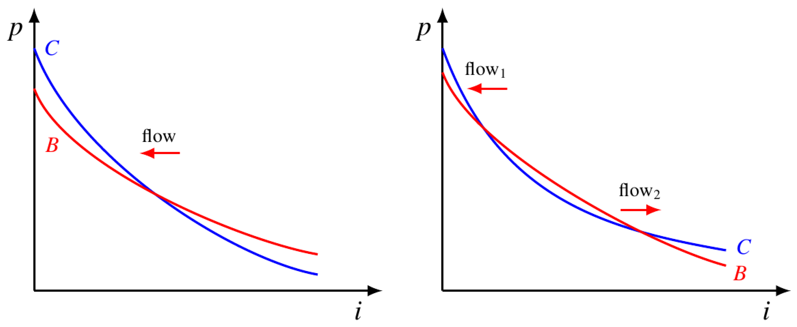
The purpose of the monotonicity property is to ensure that, given a pair of distributions C, $B\in {\mathcal{C}}_N$, the one with more cumulated weights will not be assigned a larger effective number. To formulate the requirement, it is important to realize that all C, B cannot be readily compared by the degree of their cumulation. In the left panel of Figure 3, we show an example of a comparable pair. For this purpose, weight entries were ordered in a decreasing manner so that the cumulation center is on the left. Distribution C is more cumulated since it can be obtained from B by transfer of weight (flow) directed toward the cumulation center at all times. On the other hand, the distributions shown in the right panel cannot be compared without introducing ad hoc assumptions, since flow in both directions is needed to perform the needed deformation. Thus, the universal notion of monotonicity is only concerned with properly treating the situation on the left.

It is straightforward to check that, for any pair of such comparable discrete distributions, the deformation in question can be carried out as a finite sequence of pairwise weight exchanges, each transferring weight toward the center of cumulation. Since performing such an elementary operation on C produces $C^{\prime }$, such that (C, $C^{\prime }$) is a comparable pair, the monotonicity requirement is entirely captured by the set of conditions concerning these elementary operations, namely,

$$\mathcal{N}(\dots c_i-\epsilon \dots c_j+\epsilon \dots )\le \mathcal{N}(\dots c_i\dots c_j\dots ),\forall c_i\le c_j,\forall \epsilon :0\le \epsilon \le c_i$$

M⁻

(M⁻) monotonicity is designed to identify functions respecting cumulation. To place its meaning in a more conventional context, we point out that imposing it in conjunction with symmetry (S) (see below) results in a well-known property of Schur concavity [6].

2.3. Effective-Number Functions

Apart from additivity (A) and monotonicity (M⁻), the axioms defining effective-number functions $\mathcal{N}=\mathcal{N}\left[C\right]$ incorporate intuitive and easily formulated features such as symmetry, continuity, and previously mentioned “boundary values” associated with uniform and $\delta$-function distributions. The complete list of these additional requirements is formally specified below.

$$\mathcal{N}(\dots c_i\dots c_j\dots )=\mathcal{N}(\dots c_j\dots c_i\dots ),\forall i\ne j$$

(S)

$$\mathcal{N}=\mathcal{N}\left[C\right]\mathrm{is}\mathrm{continuous}\mathrm{on}{\mathcal{C}}_N,\forall N$$

(C)

$$\mathcal{N}(1,1,\dots ,1)=N,(1,1,\dots ,1)\in {\mathcal{C}}_N,\forall N$$

(B1)

$$\mathcal{N}(N,0,\dots ,0)=1,(N,0,\dots ,0)\in {\mathcal{C}}_N,\forall N$$

(B2)

$$1\le \mathcal{N}\left[C\right]\le N,\forall C\in {\mathcal{C}}_N,\forall N$$

(B)

It can be shown that (B1) and (B) follow from the remaining five requirements, leading to a definition of ENF set $\mathfrak{N}$ as a collection of real-valued functions $\mathcal{N}=\mathcal{N}\left[C\right]$ on $\mathcal{C}$, satisfying (A), (M₋), (S), (B2) and (C).

Each ENF contained in $\mathfrak{N}$ provides a consistent scheme to assign effective totals (effective counting measures) to sets of objects endowed with counting/probability weights. It should be pointed out in that regard that none of the quantifiers currently used as substitutes for effective numbers, such as participation number [7], exponentiated Shannon entropy [8], or exponentiated Rényi entropies [9], is (A)-additive. However, they do respect all the other axioms defining $\mathfrak{N}$.

2.4. Minimal Amount

Interestingly, effective-number theory based on the above definition of $\mathfrak{N}$ can be entirely solved [3]. In fact, all ENFs were explicitly found, and the structural properties of $\mathfrak{N}$ were established. These results are summarized by Theorems 1 and 2 of Reference [3]. To convey the aspects needed here, we first defined function ${\mathcal{N}}_{+}$ on $\mathcal{C}$, counting the number of objects with nonzero weights, namely,

$${\mathcal{N}}_{+}\left[C\right]=\sum _{i=1}^N{\mathrm{n}}_{+}\left(c_i\right){\mathrm{n}}_{+}\left(c\right)=\left\{\begin{array}{cc}0,\hfill & c=0\hfill \\ 1,\hfill & c>0\hfill \end{array}\right.$$

(6)

Note that ${\mathcal{N}}_{+}$ is not an ENF due to the lack of continuity. In addition, the following function ${\mathcal{N}}_{★}$ on $\mathcal{C}$ is important in the context of effective-number theory and the below theorem.

$${\mathcal{N}}_{★}\left[C\right]=\sum _{i=1}^N{\mathfrak{n}}_{★}\left(c_i\right){\mathfrak{n}}_{★}\left(c\right)=min\{c,1\}$$

(7)

Theorem 1.

There are infinitely many elements in $\mathfrak{N}$ including ${\mathcal{N}}_{★}$. Moreover, for every fixed $C\in \mathcal{C}$,

$$\left\{\mathcal{N}\left[C\right]\mid \mathcal{N}\in \mathfrak{N}\right\}=\left\{x\in \mathbb{R}\mid {\mathcal{N}}_{★}\left[C\right]\le x\le {\mathcal{N}}_{+}\left[C\right]\right\}$$

(8)

We wish to emphasize the following points regarding this theorem.

(a) Since $\mathfrak{N}$ is nonempty, the set of all possible effective-number assignments for a given counting vector C (LHS of (8)) is also nonempty, and thus equal to closed interval $[{\mathcal{N}}_{★}\left[C\right],{\mathcal{N}}_{+}\left[C\right]]$. (As shown in Reference [3], this closed interval shrinks to a single point $\{{\mathcal{N}}_{★}\left[C\right]={\mathcal{N}}_{+}\left[C\right]\}$ iff C is such that $c_i\notin (0,1),\forall i$.)

(b) It follows from Equation (8) that

$${\mathcal{N}}_{★}\left[C\right]\le \mathcal{N}\left[C\right]\le {\mathcal{N}}_{+}\left[C\right],\forall \mathcal{N}\in \mathfrak{N},\forall C\in \mathcal{C}$$

(9)

Thus, the concept of effective counting measure necessitates the existence of a nontrivial intrinsic minimal amount (count, total), specified by ${\mathcal{N}}_{★}$. Universal (independent of N) function ${\mathfrak{n}}_{★}$ entering Definition (7) of this minimal ENF is referred to as the minimal counting function. This result has nontrivial consequences, including those concerning quantum uncertainty discussed here.

(c) In addition, the theorem conveys that ${\mathcal{N}}_{★}$ is the only ENF with such definite structural role in $\mathfrak{N}$. For example, since ${\mathcal{N}}_{+}\notin \mathfrak{N}$, there is no larger element in $\mathfrak{N}$, i.e., the analog of ${\mathcal{N}}_{★}$ “at the top”. More importantly, for a given C, function $\mathcal{N}$ can be adjusted to accommodate any intuitively possible total larger than ${\mathcal{N}}_{★}\left[C\right]$. Consequently, there are no “holes” in the bulk of $\mathfrak{N}$ where other privileged ENFs could be identified. Given its absolute meaning, minimal amount ${\mathcal{N}}_{★}$ provides for the canonical solution of quantum-identity Problem (1). In particular [3],

$$\mid \psi \rangle ,\left\{\mid i\rangle \right\}⟶{\mathcal{N}}_{★}[\mid \psi \rangle ,\left\{\mid i\rangle \right\}]={\mathcal{N}}_{★}\left[C\right],c_i=N\mid \langle i\mid \psi \rangle {\mid }^2$$

(10)

3. Measure Aspect of Quantum Uncertainty

Uncertainty in QM refers to the indeterminacy of outcomes obtained by probing the quantum state. More specifically, consider a canonical situation where state $\mid \psi \rangle$ from N-dimensional Hilbert space is probed by measuring the observable associated with nondegenerate Hermitian operator $\widehat{O}$. In a standard manner, $\mid \psi \rangle$ is repeatedly prepared and measured, generating a sequence of outcomes:

$$\mid \psi \rangle \stackrel{\mathrm{measure}\widehat{O}}{\to }\{(\mid i_{\ell }\rangle ,O_{i_{\ell }})\mid \ell =1,2,\dots \}$$

(11)

With $\{(\mid i\rangle ,O_i)\mid i=1,2,\dots ,N\}$ denoting the set of eigenstate–eigenvalue pairs, $(\mid i_{\ell }\rangle ,O_{i_{\ell }})$ specifies the outcome of the ℓ-th trial, namely, the collapsed state and the measured value. The quantum uncertainty of $\mid \psi \rangle$ with respect to its probing by $\widehat{O}$ is intuitively associated with the “spread” of outcomes $(\mid i_{\ell }\rangle ,O_{i_{\ell }})$ so generated.

Clearly, the precise content of the notion so construed depends on how we choose to quantify the “spread”. In the usual approach, the focus is on sequence of eigenvalues $O_{i_{\ell }}$ with a spread characterized in terms of distance (metric) on the spectrum of $\widehat{O}$. We refer to this approach as metric uncertainty ($\rho$-uncertainty). A commonly used quantifier of this type is the standard deviation that leads to a particularly simple form of quantum-uncertainty relations [1].

However, it may be interesting to view quantum indeterminacy differently [5]. A possible approach is to characterize it by the effective number of distinct outcomes occurring in Equation (11). This would express the spread in terms of the “amount”, and we refer to it as measure uncertainty ($\mu$-uncertainty). Note that, in this case, it is immaterial whether we focus on sequence $O_{i_{\ell }}$, sequence $\mid i_{\ell }\rangle$, or on the sequence of corresponding pairs: the object of interest is the effective total of the outcomes. While such an approach might have seemed rather nebulous in the past, it is clear that effective-number theory not only puts it on firm ground, but also leads to rather unexpected revelations.

First, by construction, set $\mathfrak{N}$ of ENFs is identical to the set of all possible $\mu$-uncertainties. More explicitly, if $\mu =\mu [\mid \psi \rangle ,\{\mid i\rangle \left\}\right]$ formally denotes a valid $\mu$-uncertainty map, then there exists $\mathcal{N}\in \mathfrak{N}$, such that, for all $\mid \psi \rangle$ and $\left\{\mid i\rangle \right\}$,

$$\mu [\mid \psi \rangle ,\left\{\mid i\rangle \right\}]=\mathcal{N}\left[C\right],C=(c_1,\dots ,c_N),c_i=N\mid \langle i\mid \psi \rangle {\mid }^2,$$

(12)

and vice versa. In other words, $\mu =\mu [\mid \psi \rangle ,\{\mid i\rangle \left\}\right]$ is the same object as $\mathcal{N}=\mathcal{N}[\mid \psi \rangle ,\{\mid i\rangle \left\}\right]$ featured in quantum-identity Problem (1).

Second, the existence of a minimal effective number gives rise to minimal $\mu$-uncertainty. In particular, effective-number theory allows us to deduce the following rigorous statement:

[U${}_0$]

The μ-uncertainty of $\mid \psi \rangle$ with respect to $\left\{\mid i\rangle \right\}$ is at least ${\mathcal{N}}_{★}[\mid \psi \rangle ,\left\{\mid i\rangle \right\}]$ states (Equations (7) and (10)).

Remarkably, U${}_0$ asserts that uncertainty is built into quantum mechanics as an absolute concept. In particular, by expressing it as a measure, we learn that there exists an intrinsic irremovable “amount” of uncertainty in state $\mid \psi \rangle$, relative to probing basis $\left\{\mid i\rangle \right\}$, specified uniquely as ${\mathcal{N}}_{★}[\mid \psi \rangle ,\left\{\mid i\rangle \right\}]$ states.

Note that U${}_0$ can be viewed as a quantum-uncertainty principle of a very different kind than the one conveyed by Heisenberg relations [1,4]. Indeed, while the latter is of a relative (comparative) nature, the $\mu$-uncertainty principle is absolute. It allows us to express the fundamental difference between quantum and classical notions of state in a particularly direct and economic way, represented by the following diagram:

$$\begin{array}{cc}\hfill \mathrm{classical}\mathrm{state}S& \leftrightarrow \mathrm{quantum}\mathrm{state}\mid \psi \rangle \hfill \\ \hfill S\stackrel{\mathrm{measurement}}{\to }S& \leftrightarrow \mid \psi \rangle \stackrel{\mathrm{measurement}}{\to }\mid i\rangle \hfill \\ \hfill \mu -\mathrm{uncertainty}=1\mathrm{state}& \leftrightarrow \mu -\mathrm{uncertainty}={\mathcal{N}}_{★}[\mid \psi \rangle ,\left\{\mid i\rangle \right\}]\mathrm{states}\hfill \end{array}$$

Thus, the properties of classical state S can be measured with arbitrarily small error, meaning that its intrinsic $\mu$-uncertainty is always one (S has single identity). On the other hand, if the probing of a quantum state $\mid \psi \rangle$ involves the collapse into elements of basis $\left\{\mid i\rangle \right\}$, its intrinsic $\mu$-uncertainty is ${\mathcal{N}}_{★}[\mid \psi \rangle ,\left\{\mid i\rangle \right\}]$, which is generically much larger than one ($\mid \psi \rangle$ has ${\mathcal{N}}_{★}[\mid \psi \rangle ,\left\{\mid i\rangle \right\}]$ identities).

Finally, it is important to point out that the above considerations are by no means restricted to a discrete case or finite-dimensional Hilbert spaces. The relevant extensions are worked out in complete generality by Reference [5]. As an elementary example, consider the case of a spinless Schrödinger particle contained in region $\mathrm{\Omega }\subset {\mathbb{R}}^D$ with volume V. Using the above results, one can show that its minimal $\mu$-uncertainty with respect to the position basis is given by

$${\mathcal{V}}_{★}\left[\psi \right]={\int }_{\mathrm{\Omega }}{d}^{D}xmin\{V{\psi }^{★}\left(x\right)\psi \left(x\right),1\},$$

(13)

where $\psi \left(x\right)$ is the particle’s wave function. Thus, measure uncertainty takes the form of effective volume. The corresponding $\mu$-uncertainty principle states that a particle described by $\psi$ cannot be associated with effective volume smaller than ${\mathcal{V}}_{★}\left[\psi \right]$.

4. Conclusions

In the first part of this presentation, we outlined the construction of effective-number theory and discussed how it solves the quantum-identity problem [3]. The latter has a wide range of potential applications in quantum physics. Particularly close attention was paid to the most consequential result of effective-number theory, namely, the existence of a minimal amount (total, count) consistently assignable to a collection of objects distinguished by probability weights. This finding offers a rather unexpected new insight into the nature of measure.

In the second part of the presentation, we analyzed the consequences of effective-number theory for the concept of uncertainty in quantum mechanics [5]. In particular, we argued that the ensuing measure approach reveals the existence of uniquely defined intrinsic $\mu$-uncertainties in quantum state, each associated with a particular way of probing it. We propose these intrinsic uncertainties as potentially useful characteristics of quantum states. It is interesting to note in this regard that, starting from essentially classical (measure) considerations, we arrived at describing aspects of the state that are truly quantum in their nature.