Abstract
If the Dirac magnetic monopoles exist, they can be probed in the collider experiments. Earlier, only the Drell–Yan production mechanism of magnetic monopoles was used to look for magnetic monopoles. However, the photon fusion production mechanism of magnetic monopoles is the dominant production mechanism at the LHC energy. I will discuss the photon fusion production of spin 0, 1/2, and 1 monopoles using the MadGraph event generator. I will also show the kinematic distributions of magnetic monopoles having those three spins. The comparison between the Drell–Yan process and the photon fusion process will also be done.
1. Introduction
In 1931, Dirac [1] gave a concrete formulation of magnetic monopoles as a quantum mechanical source of magnetic poles. Yet, today, the magnetic monopole remains a hypothetical particle. Dirac conceived of the monopole as a point-like particle. Its spin and mass are not determined by theory.
Since monopoles are yet to be found, many experiments have searched or are searching for this object. Most collider experiments considered only the Drell–Yan (DY) production mechanism of the monopole production in order to search for magnetic monopoles. However, in the collider energy of the LHC, the cross-section for the monopole production mechanism of Photon Fusion (PF) is higher than that of the DY production mechanism [2].
In previous searches for CDF [3], ATLAS [4,5], and MoEDAL [6,7] experiments, different monopole models of the DY production mechanism were simulated using MadGraph [8,9]. It should be stressed that due to the large coupling constant between the photon and monopole, the perturbative calculation is not possible. Therefore, only tree-level Feynman-like diagrams of DY have been repeatedly used in extracting monopole mass limits in collider experiments.
Since the collider experiments will extend the search for magnetic monopoles using the PF mechanism along with the DY mechanism, it is important that the PF mechanism also be implemented through MadGraph. In this report, a brief description of the implementation of the PF mechanism in MadGraph is given. This report is based on the paper [10] describing the PF MadGraph models.
2. MadGraph Universal FeynRules Output Model
The DY production mechanism was implemented in MadGraph using the Fortran code setup. However, this implementation was inadequate to describe the bosonic monopole production, as it requires a four-particle vertex in the tree level calculation. The PF mechanism was implemented though the Universal FeynRules Output (UFO) model of MadGraph [11].
2.1. Monopole Couplings
In Dirac’s magnetic monopole model, the relation between the elementary electric charge () and the basic magnetic charge (g) is given by:
Here, Heaviside–Lorentz units have been used, the convention followed by MadGraph. Hence, from Equation (1), the unit of magnetic charge is:
In Heaviside–Lorentz units, the electromagnetic vertex is . Similarly, in these units, the monopole-photon coupling becomes . The electric charge is given by where is the fine structure constant. Then, from Equation (2), one gets:
In Equation (3), the monopole velocity has not been used. However, if one considers the photon-monopole coupling to be -dependent, then the value of simply becomes . The velocity can be found from the Mass (M) of the monopole using the following equation:
where is the square of the center-of-mass energy of the colliding particles.
Here, it should be mentioned that the presence of velocity in photon-monopole coupling is debated. If one follows the symmetry argument of the electron and monopole, the photon-monopole coupling should not be velocity dependent as photon-electron coupling is not velocity dependent. However, Milton [12] described the monopole-electron scattering. By comparing the expressions with Rutherford scattering, he found that the photon-monopole coupling is velocity dependent. Here, we follow an agnostic approach, i.e., simulate the production of monopoles with both velocity-dependent and -independent coupling.
2.2. Generation and Validation of the MadGraph UFO Model
The FeynRules interface [13] for the Mathematica package has been used to generate the UFO models. Here, the parameters of a model (i.e., masses of particles, spins, electric charges, magnetic charges, coupling constants, etc.) and the corresponding Lagrangian are written to a text file in a way that Mathematica can understand the variables. FeynRules generates the UFO model from that text file.
The is defined as a form factor to the coupling [14]. The value of has been obtained from the following equation:
Here, and are the four-momentum of the two colliding particles.
To generate the UFO model, one needs to feed the Lagrangian to the FeynRules. Therefore, the UFO model for the scalar monopole was generated by using this Lagrangian [10]:
where is the photon field, whose field strength tensor is given by and is the scalar monopole field. Here, is simply g for -independent photon-monopole coupling and for -dependent coupling, is .
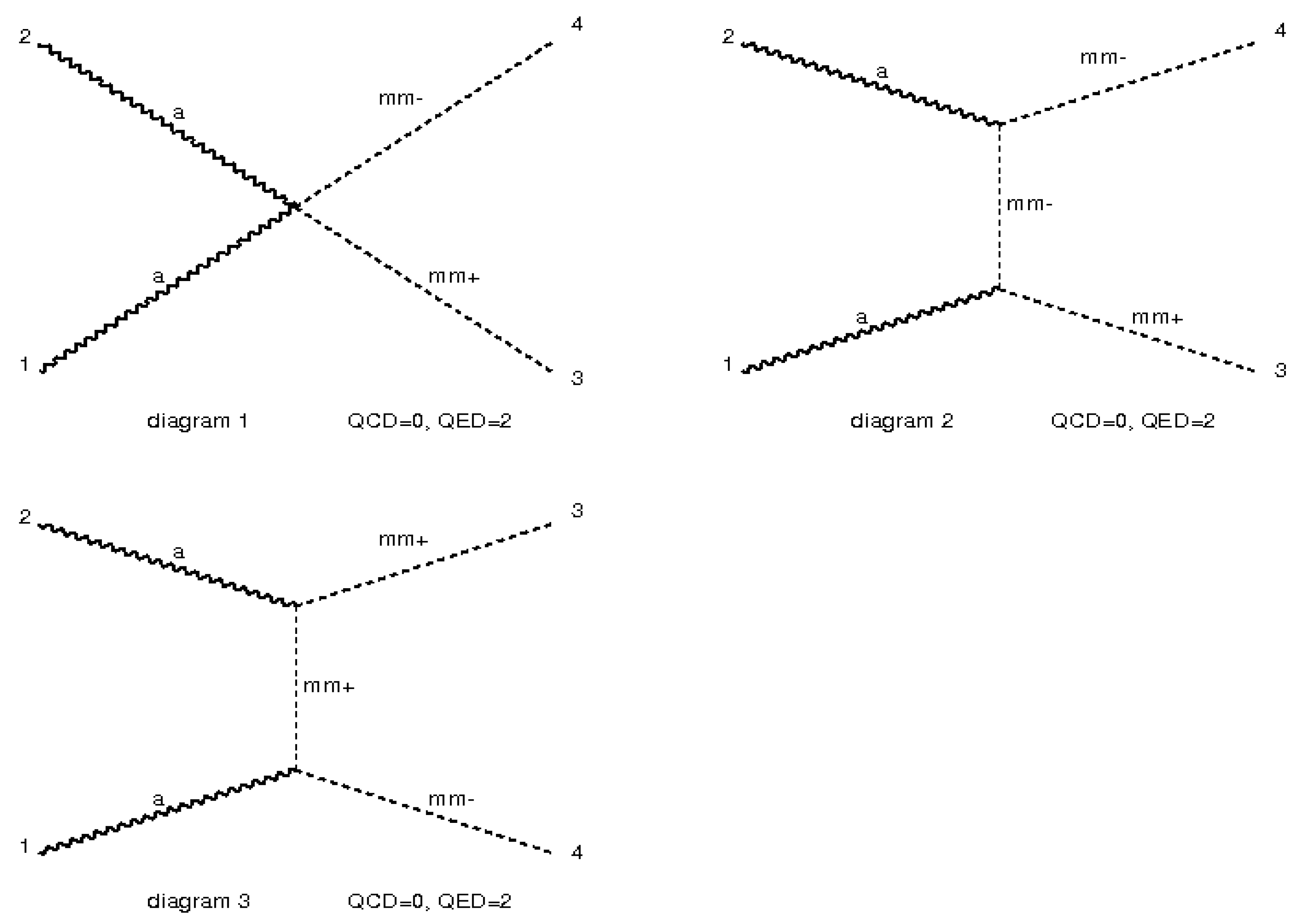
Once generated, the UFO model needs to be validated. This was done by comparing the cross-sections from the theoretical predictions and the cross-sections obtained from MadGraph, when no Parton Distribution Function (PDF)was used. The Feynman diagrams from the spin 0 UFO model is shown in Figure 1. The cross-section values for the -independent coupling are shown in Table 1.
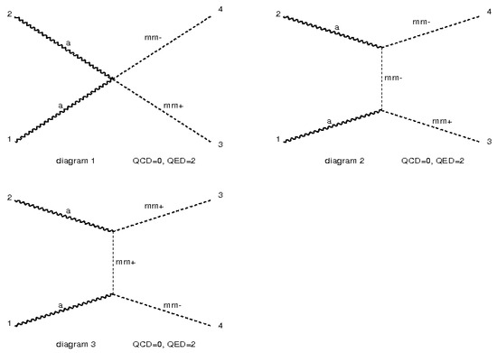
Figure 1.
The Feynman Diagram produced by MadGraph for the spin 0 magnetic monopole scenario. Here, “mm+” suggests monopole, “mm-” shows the anti-monopole, and “a” describes the photon.

Table 1.
The cross-section for the spin 0 monopole as obtained by the theory and the MadGraph UFO model for the -independent coupling when no PDF is used and the center-of-mass energy is 13 TeV. The fourth column shows the ratio of the cross-sections of the UFO model to that of the theoretical prediction. These ratios are very close to 1, suggesting excellent agreement between the theory and the MadGraph model [10].
In a similar fashion, the -dependent coupling model was compared with the theory. The cross-section values are compared in Table 2. The ratio of cross-sections for the -dependent coupling to the -independent coupling should be of the order of . This was confirmed in the sixth column of Table 2.
Table 2.
The cross-section for the spin 0 monopole as obtained by the theory and the MadGraph UFO model for the -dependent coupling constant, when no PDF is used and the center-of-mass energy is 13 TeV. The fourth column shows the ratio of the cross-sections of the UFO model to that of the theoretical prediction. These ratios are very close to 1, suggesting excellent agreement between the theory and the MadGraph model. Here, the sixth column shows the ratio of cross-sections as obtained by the UFO model for -dependent coupling to -independent coupling (shown in Table 1). This ratio varies as , as expected from the theory [10].
Similarly, the spin ½ monopole model was validated by comparing the cross-sections with the theoretical predictions with no PDF and the center-of-mass energy of 13 TeV. Here, the Lagrangian is in the following equation [10]:
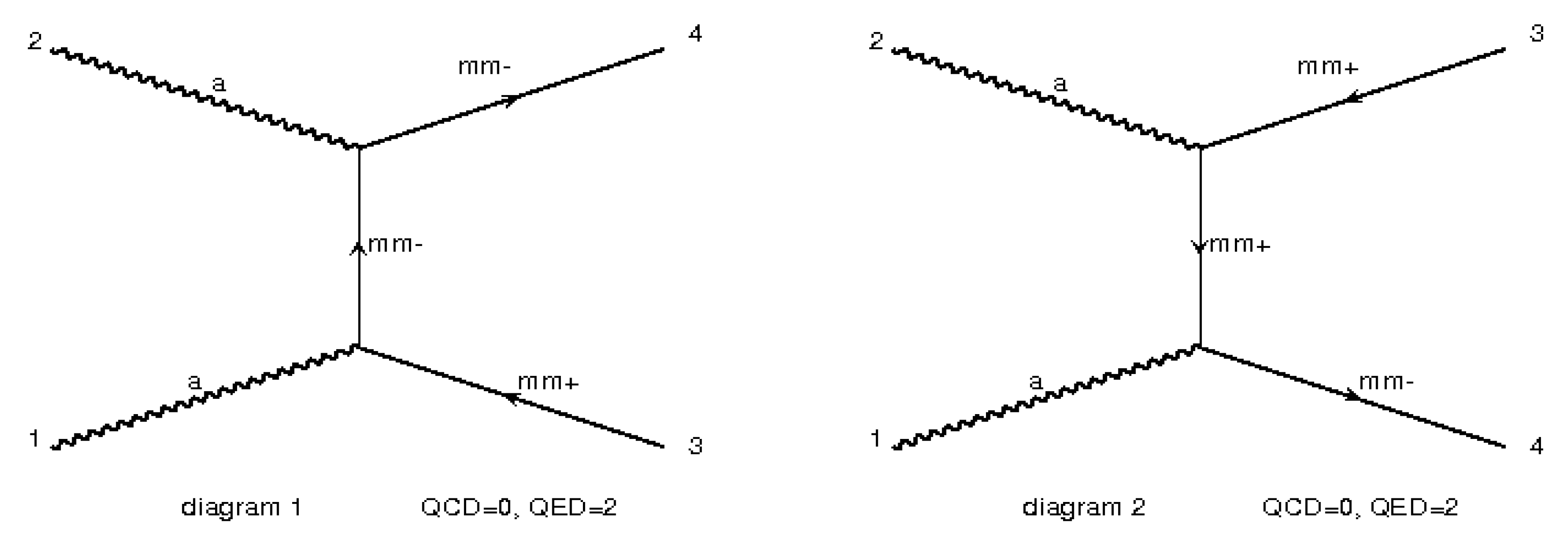
where is the electromagnetic field tensor, is the total derivative, and a commutator of the matrices is given by . The last term in the above Lagrangian is a magnetic moment-generating term [10]. Unless otherwise stated, the value of for spin ½ monopoles is taken to be zero. The diagrams considered for spin ½ are shown in Figure 2.
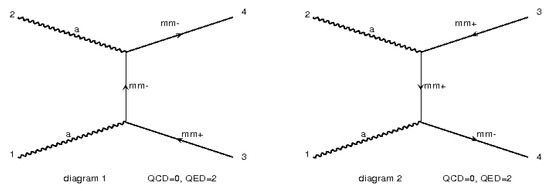
Figure 2.
The Feynman Diagrams produced by MadGraph for spin ½ magnetic monopoles. Here, “mm+” suggests monopole, “mm−” shows the anti-monopole and “a” describes the photon.
The cross-sections comparisons are shown in Table 3 (for -independent coupling) and Table 4 (for -dependent coupling). The ratios of the cross-sections of the UFO model and the theoretical predictions are very close to one. This means that the spin ½ UFO model is also well-modeled.
Table 3.
The cross-section for the spin ½ monopole as obtained by the theory and the MadGraph UFO model for the -independent coupling when no PDF is used and the center-of-mass energy is 13 TeV. The fourth column shows the ratio of the cross-sections of the UFO model to that of the theoretical prediction. As the ratios are very close to 1, this suggests excellent agreement between the theory and the MadGraph model [10].
Table 4.
The cross-section for the spin ½ monopole as obtained by the theory and the MadGraph UFO model for the -dependent coupling constant, when no PDF is used and the center-of-mass energy is 13 TeV. The fourth column shows the ratio of the cross-sections of the UFO model to that of the theoretical prediction. As these ratios are very close to 1, they suggest excellent agreement between the theory and the MadGraph model. Here, the sixth column shows the ratio of cross-sections as obtained by the UFO model for -dependent coupling to -independent coupling (shown in Table 3). This ratio varies as , as expected from the theory [10].
The cross-section ratios for -dependent coupling to -independent coupling are also shown in Table 4. These ratios are very close to , suggesting that the -dependence in the coupling has been well-modeled, as well.
After the spin 0 and spin ½ monopole models, we look at the spin 1 magnetic monopole scenario. Here, the Lagrangian is given by the following equation [10]:
Here, the tensor represents the Abelian electromagnetic field strength. The is with , the covariant derivative of , providing the coupling of the magnetically-charged vector field to the gauge field . This plays the role of the ordinary photon. The last term is the magnetic moment term, proportional to , to keep the discussion general [10]. Unless otherwise stated, the default value of for the spin 1 monopole is taken to be one.
The Feynman diagrams as generated by MadGraph for the spin 1 magnetic monopole model is shown in Figure 3. Just like the spin 0 and spin ½ magnetic monopole models, we compare the cross-sections obtained by spin 1 UFO model with the predictions from the theory. The comparisons are shown in Table 5 (for -independent coupling) and Table 6 (for -dependent coupling). This was done with no PDF and a center-of-mass energy of 13 TeV. The tables show that the cross-sections obtained by the spin 1 magnetic monopole UFO model are in excellent agreement with the theoretical predictions for both the -independent and -dependent coupling cases.
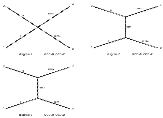
Figure 3.
The Feynman Diagrams produced by MadGraph for the spin 1 magnetic monopoles. Here “mm+” suggests monopole, “mm−” shows the anti-monopole, and “a” describes the photon.
Table 5.
The cross-section for the spin 1 monopole as obtained by the theory and the MadGraph UFO model for the -independent coupling when no PDF is used and the center-of-mass energy is 13 TeV. The fourth column shows the ratio of the cross-sections of the UFO model to that of the theoretical prediction. The ratios, being very close to 1, suggest excellent agreement between the theory and the MadGraph model [10].
Table 6.
The cross-section for the spin 1 monopole as obtained by the theory and the MadGraph UFO model for the -dependent coupling constant, when no PDF was used and the center-of-mass energy is 13 TeV. The fourth column shows the ratio of the cross-sections of UFO model to that of the theoretical prediction. The ratios, being very close to 1, suggest excellent agreement between the theory and the MadGraph model. Here, the sixth column shows the ratio of cross-sections as obtained by the UFO model for -dependent coupling to -independent coupling (shown in Table 5). This ratio varies as , as expected from the theory [10].
2.3. LHC Phenomenology
After we validate the MadGraph UFO model, we need to look at the kinematic and angular distributions of PF process and compare them with the DY process. This is an important aspect for the monopole searches at the collider experiments as the geometrical acceptance and efficiency of a detector is not uniform in the solid angle around the interaction point.
2.3.1. Kinematic Distributions
Since the monopole search results in the collider experiments have been interpreted using the DY production process, we need to compare the kinematic and angular distributions of DY and PF processes and identify the differences. In order to compare the kinematic and angular distributions of the PF and DY method, PDFs were used to get meaningful distributions. For the DY method, the PDF was set to NNPDF23 at lowest order (LO) [15]. For the PF method, LUXqed [16] was used. This was done as LUXqed provides a relatively small uncertainty in the photon distribution function of the proton [17]. For spin ½ plots, the value of the parameter was taken to be zero, and for spin 1 plots, the value of the parameter was taken to be one.
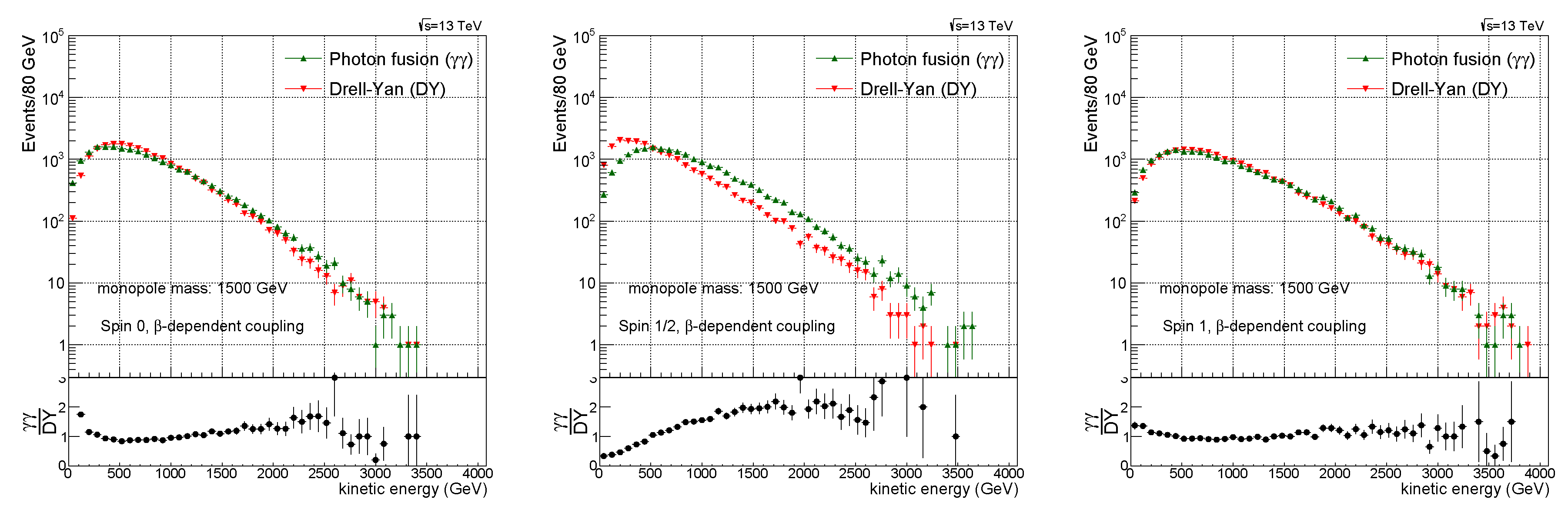
The kinetic energy distribution comparison between PF and DY processes is shown in Figure 4. The pseudorapidity distribution () comparison is shown in Figure 5.
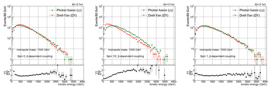
Figure 4.
Kinetic energy distribution comparison between the photon fusion and Drell–Yan processes for spin 0 (left), spin ½ (middle), and spin 1 (right) monopoles. Here, -dependent coupling has been used. For the PDFs, NNPDF23 was used for the Drell–Yan process and LUXqed was used for the photon fusion process [10].
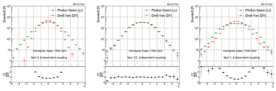
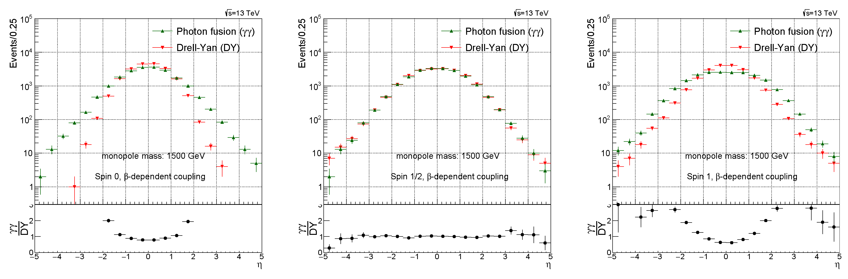
Figure 5.
Pseudorapidity () distribution comparison between the photon fusion and Drell–Yan processes for spin 0 (left), spin ½ (middle), and spin 1 (right) monopoles. Here, -dependent coupling has been used. For the PDFs, NNPDF23 was used for the Drell–Yan process and LUXqed was used for the photon fusion process [10].
2.3.2. Limiting Case of Large and Small for Photon Fusion
In this section, we want to see the cross-section and kinematic distributions of the PF process for the large and small scenario for the spin ½ and 1 monopole cases. If the cross-section is finite at this limit, then this may open a way to potential perturbatively-consistent search in colliders.
a. Spin ½ monopole scenario: A magnetic moment-generating term has been added to the Lagrangian of the spin ½ monopole case (Equation (7)). A dimensionless parameter with M being the mass of the monopole has been varied from 0–10,000 for the photon fusion process with a photon-photon collision energy of 13 TeV. The cross-section for (the Standard Model scenario) goes to zero at very fast, as can be seen from the third column of Table 7. However, for the non-zero , the cross-section values remain finite, even if the goes to zero. The same conclusion can be obtained from the left plot of Figure 6, where the cross-section has been plotted against the monopole mass for the proton-proton collision energy of 13 TeV.
Table 7.
Photon fusion production cross-sections at a photon-photon collision energy of 13 TeV for the spin ½ monopole, -dependent coupling, and various values of the parameter [10].
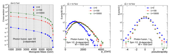
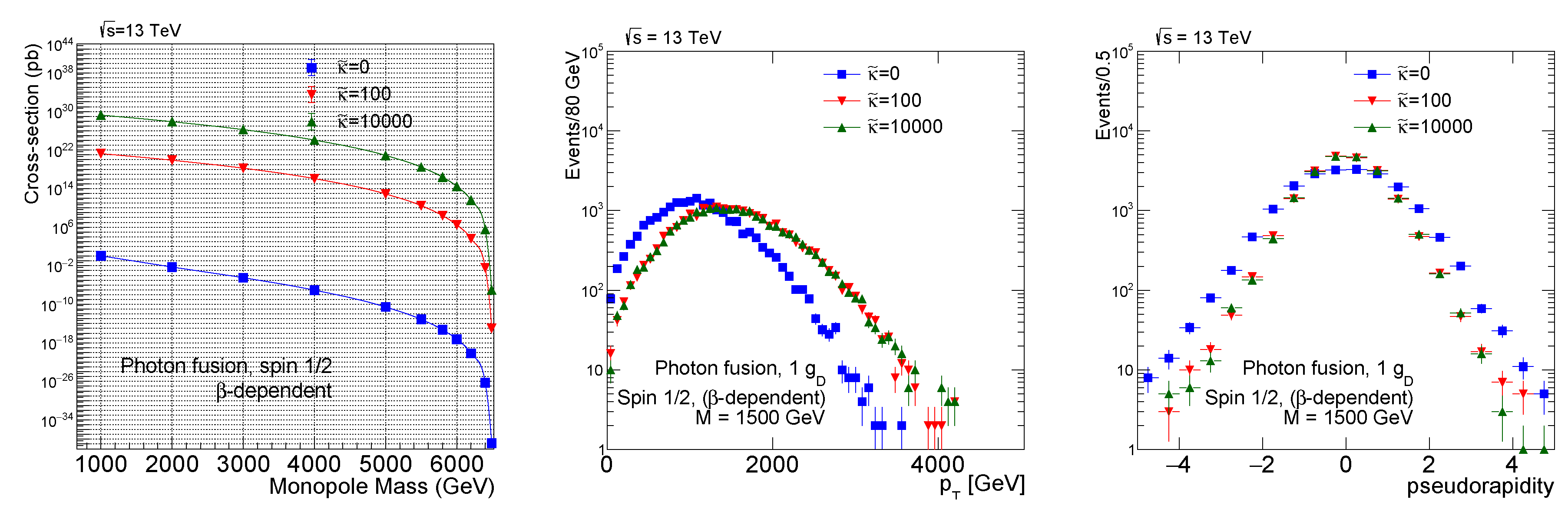
Figure 6.
The cross-section variation with the monopole mass at a proton-proton collision energy of 13 TeV is shown on the left plot for the spin ½ monopoles. The transverse momentum () distribution (middle) and pseudorapidity distribution (right) are shown for the spin ½ monopole at a proton-proton collision energy of 13 TeV [10].
The central and right-hand side plots of Figure 6 show the transverse momentum distribution and pseudorapidity distribution for different scenarios. Here, shows the Standard Model case. The spectrum is harder than the Standard Model case when . The pseudorapidity distribution is more central for than the Standard Model case of .
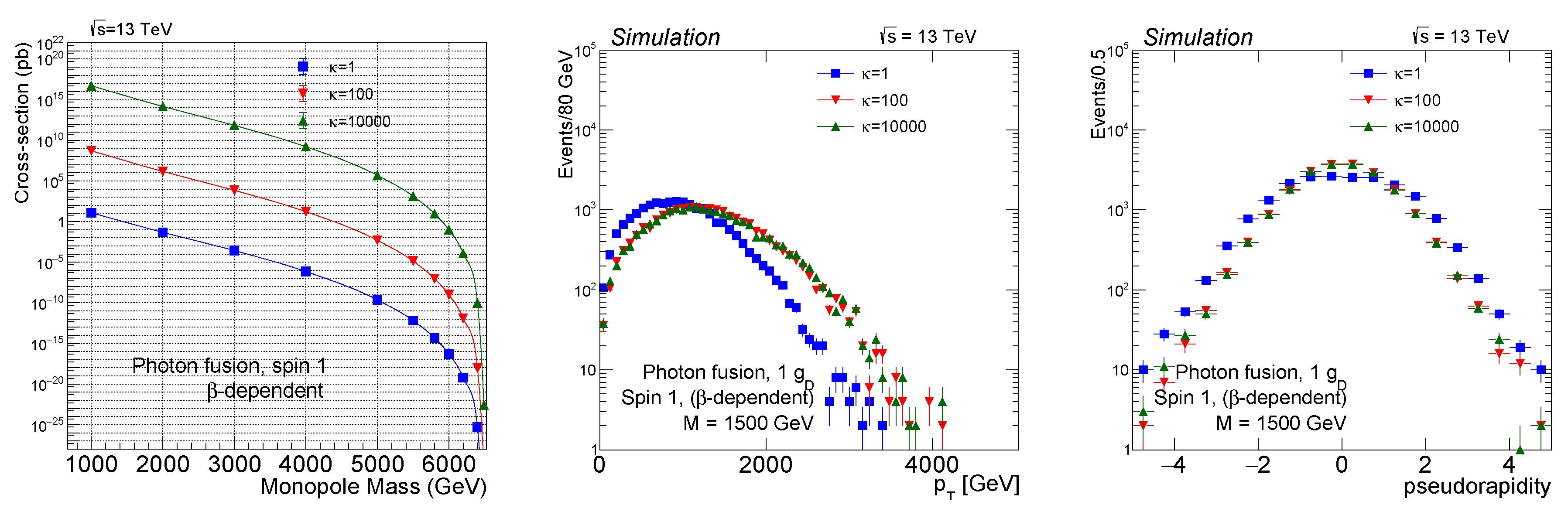
b. Spin 1 monopole scenario: Similar to the spin ½ monopole scenario, the spin 1 monopole also has a magnetic moment term in the Lagrangian (Equation (8)). For the spin 1 monopole, is the Standard Model case. Here, the cross-section for the case goes to zero very fast as goes to zero (as seen from the third column of Table 8) at a photon-photon collision energy of 13 TeV. However, when , the cross-section remains finite as goes to zero. A similar conclusion can be drawn from the cross-section vs. monopole mass plot of Figure 7 (left), where the proton-proton collision energy of 13 TeV has been used.
Table 8.
Photon fusion production cross-sections at a photon-photon collision energy of 13 TeV for the spin 1 monopole, -dependent coupling, and various values of the parameter [10].
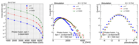
Figure 7.
The cross-section variation with the monopole mass at a proton-proton collision energy of 13 TeV is shown on the left plot for the spin 1 monopoles. The transverse momentum () distribution (middle) and pseudorapidity distribution (right) are shown for the spin 1 monopole at a proton-proton collision energy of 13 TeV [10].
The transverse momentum distribution and the pseudorapidity distribution have been compared for different values of for the spin 1 monopole case at the proton-proton collision energy of 13 TeV and are shown in the central and right plots of Figure 7. Here, similar to the spin ½ scenario, models with values yield a spectrum harder than the Standard Model scenario when . The pseudorapidity distribution is more central for than the Standard Model case of .
3. Conclusions
In this report, an overview of the phenomenological study of magnetic monopoles with the help of MadGraph models is given. In the first part, the details of the generation of MadGraph UFO models were described. Subsequently, those models were successfully validated by checking the cross-section values given by the models against the theoretical predictions.
In the second part, the LHC phenomenology of these models was described. The kinetic energy and pseudorapidity distribution comparisons between the DY method and PF method have been shown. Furthermore, a potential perturbative limit was given when was high, but monopole velocity was very low. In that limit, the cross-sections for the spin ½ and spin 1 monopoles were finite. This proceeding also showed the kinetic and pseudorapidity distribution comparisons for different values for the spin ½ and spin 1 monopoles.
The UFO models can be used by the collider experiments to simulate the photon fusion production mechanism of magnetic monopoles. The MoEDAL experiment at the LHC is using these models to interpret its latest data. The MoEDAL paper is in preparation.
Funding
The author acknowledges the support by the Generalitat Valenciana (GV) through the MoEDAL- supporting agreements, by the Spanish MINECO under the project FPA2015-65652-C4-1-R, and by the Severo Ochoa Excellence Centre Project SEV-2014-0398.
Acknowledgments
The author would like to thank Wendy Taylor, Manoj Kumar Mondal, and Olivier Mattelaer for discussions on the MadGraph implementation, as well as fellow colleagues from the MoEDAL-LHC Collaboration for their interest.
Conflicts of Interest
The author declares no conflict of interest. The funding sponsors had no role in the design of the study; in the collection, analyses, or interpretation of the data; in the writing of the manuscript; nor in the decision to publish the results.
Abbreviations
The following abbreviations are used in this manuscript:
| LHC | Large Hadron Collider |
| ATLAS | A Toroidal LHC Apparatus |
| MoEDAL | Monopole and Exotics Detector at the LHC |
| PF | Photon Fusion |
| DY | Drell–Yan |
| UFO | Universal FeynRules Output |
References
- Dirac, P.A.M. Quantised singularities in the electromagnetic field. Proc. R. Soc. Lond. A 1931, 133, 60. [Google Scholar]
- Dougall, T.; Wick, S.D. Dirac magnetic monopole production from photon fusion in proton collisions. Eur. Phys. J. A 2009, 39, 213. [Google Scholar] [CrossRef]
- Abulencia, A.; Acosta, D.; Adelman, J.; Affolder, T.; Akimoto, T.; Albrow, M.G.; Ambrose, D.; Amerio, S.; Amidei, D.; Anastassov, A.; et al. [CDF Collaboration]. Direct search for Dirac magnetic monopoles in pp¯ collisions at s=1.96 TeV”. Phys. Rev. Lett. 2006, 96, 201801. [Google Scholar] [CrossRef] [PubMed]
- Aad, G.; Abajyan, T.; Abbott, B.; Abdallah, J.; Khalek, S.A.; Abdelalim, A.A.; Abdinov, O.; Aben, R.; Abi, B.; Abolins, M.; et al. [ATLAS Collaboration]. Search for Magnetic Monopoles in s=7 TeV pp Collisions with the ATLAS Detector. Phys. Rev. Lett. 2012, 109, 261803. [Google Scholar] [CrossRef] [PubMed]
- Aad, G.; Abbott, B.; Abdallah, J.; Abdinov, O.; Aben, R.; Abolins, M.; AbouZeid, O.S.; Abramowicz, H.; Abreu, H.; Abreu, R.; et al. [ATLAS Collaboration]. Search for magnetic monopoles and stable particles with high electric charges in 8 TeV pp collisions with the ATLAS detector. Phys. Rev. D 2016, 93, 052009. [Google Scholar] [CrossRef]
- Acharya, B.; Alexandre, J.; Baines, S.; Benes, P.; Bergmann, B.; Bernabéu, J.; Branzas, H.; Campbell, M.; Caramete, L.; Cecchini, S.; et al. [MoEDAL Collaboration]. Search for Magnetic Monopoles with the MoEDAL Forward Trapping Detector in 13 TeV Proton-Proton Collisions at the LHC. Phys. Rev. Lett. 2017, 118, 061801. [Google Scholar] [CrossRef] [PubMed]
- Acharya, B.; Alexandre, J.; Baines, S.; Benes, P.; Bergmann, B.; Bernabéu, J.; Bevan, A.; Branzas, H.; Campbell, M.; Caramete, L.; et al. [MoEDAL Collaboration]. Search for magnetic monopoles with the MoEDAL forward trapping detector in 2.11 fb-1 of 13 TeV proton-proton collisions at the LHC. Phys. Lett. B 2018, 782, 510. [Google Scholar] [CrossRef]
- Alwall, J.; Herquet, M.; Maltoni, F.; Mattelaer, O.; Stelzer, T. MadGraph 5: Going Beyond. J. High Energy Phys. 2011, 1106, 128. [Google Scholar] [CrossRef]
- MadGraph Website. Available online: https://launchpad.net/mg5amcnlo (accessed on 24 May 2017).
- Baines, S.; Mavromatos, N.E.; Mitsou, V.A.; Pinfold, J.; Santra, A. Monopole production via photon fusion and Drell–Yan processes: MadGraph implementation and perturbativity via velocity-dependent coupling and magnetic moment as novel features. Eur. Phys. J. C 2018, 78, 966. [Google Scholar] [CrossRef] [PubMed]
- Degrande, C.; Duhr, C.; Fuks, B.; Grellscheid, D.; Mattelaer, O.; Reiter, T. UFO - The Universal FeynRules Output. Comput. Phys. Commun. 2012, 183, 1201. [Google Scholar] [CrossRef]
- Milton, K.A. Theoretical and experimental status of magnetic monopoles. Rept. Prog. Phys. 2006, 69, 1637–1712. [Google Scholar] [CrossRef]
- FeynRules Website. Available online: http://feynrules.irmp.ucl.ac.be/ (accessed on 29 September 2017).
- MadGraph Formfactor Website. Available online: https://cp3.irmp.ucl.ac.be/projects/madgraph/wiki/FormFactors (accessed on 8 October 2017).
- Ball, R.D.; Bertone, V.; Carrazza, S.; Deans, C.S.; Debbio, L.D.; Forte, S.; Guffanti, A.; Hartland, N.P.; Latorre, J.I.; Rojo, J.; et al. Parton distributions with LHC data. Nucl. Phys. B 2013, 867, 244. [Google Scholar] [CrossRef]
- Manohar, A.; Nason, P.; Salam, G.P.; Zanderighi, G. How Bright is the Proton? A Precise Determination of the Photon Parton Distribution Function. Phys. Rev. Lett. 2016, 117, 242002. [Google Scholar] [CrossRef] [PubMed]
- Manohar, A.V.; Nason, P.; Salam, G.P.; Zanderighi, G. The photon content of the proton. J. High Energy Phys. 2017, 1712, 046. [Google Scholar] [CrossRef]

Publisher’s Note: MDPI stays neutral with regard to jurisdictional claims in published maps and institutional affiliations. |
© 2019 by the author. Licensee MDPI, Basel, Switzerland. This article is an open access article distributed under the terms and conditions of the Creative Commons Attribution (CC BY) license (https://creativecommons.org/licenses/by/4.0/).