Improved Event Mixing for Resonance Yield Extraction ^†

Abstract

Resonance particles, such as the K*(892) meson, are reconstructed from the invariant mass (M${}_{inv}$) distribution of possible particle pairs. To extract the yield with the highest precision, the combinatorial background must be determined as precisely as possible. An event-mixed M${}_{inv}$ distribution is often used to describe the combinatorial background. However, this distribution will not contain the mini-jet-like structures present inside an event. This analysis introduces a new re-weighing scheme, where two M${}_{inv}$ distributions of like-sign particles in the same-event and in mixed-events are used to correct the mixed-event background estimate for the mini-jet-like structure. Using PYTHIA 8.2 generated proton-proton collisions at $\sqrt{s_{\mathrm{NN}}}$ = 5.02 TeV, it is shown that the new method can be used to more accurately describe the combinatorial background.

1. Introduction

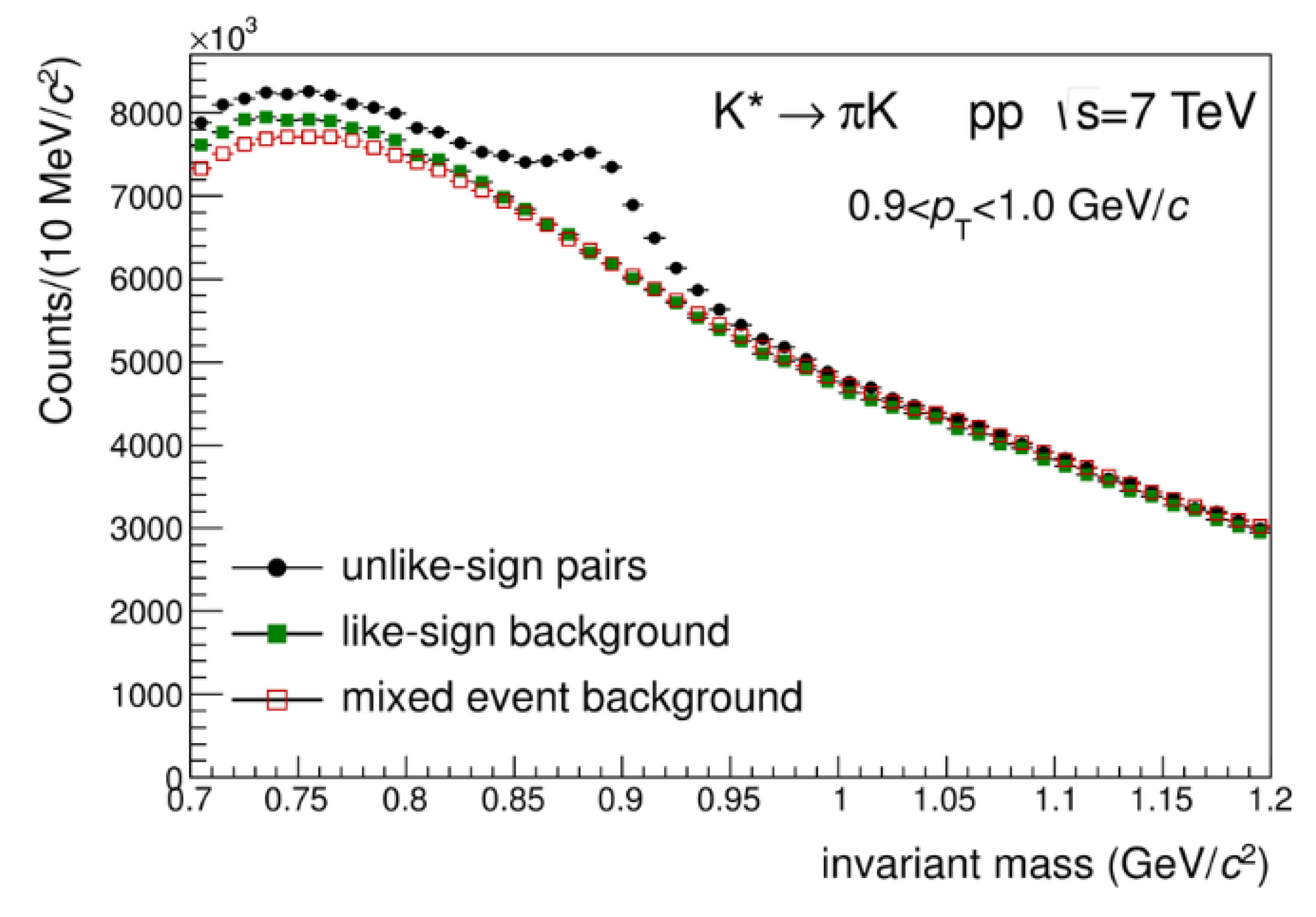
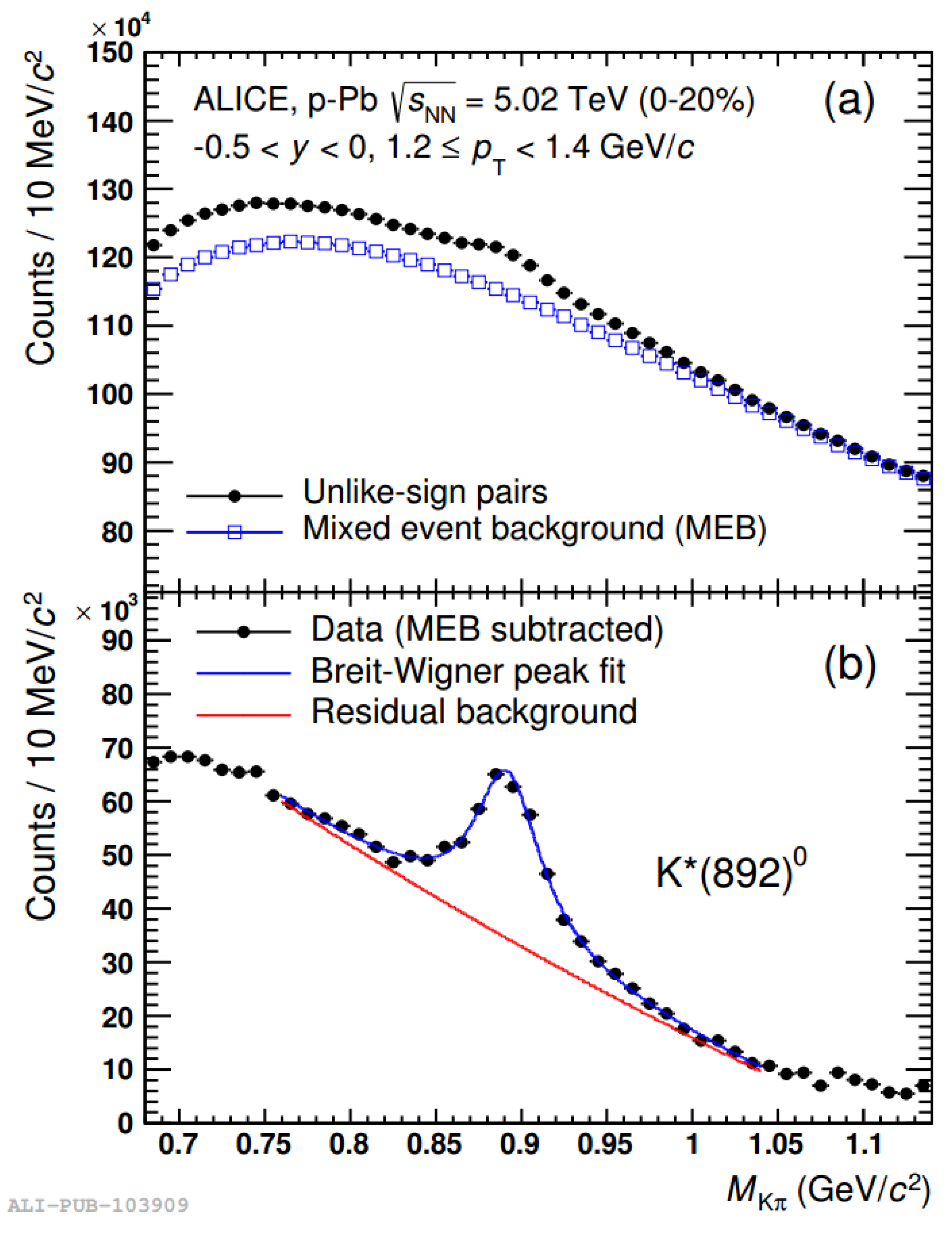
Resonance particles, such as the K*(892) meson, are produced as intermediary states in high-energy hadronic collisions. It is not possible to directly detect resonance particles due to their short life-times. Instead, the resonance particle has to be reconstructed by measuring the invariant mass (M${}_{inv}$) of its decay constituents. As it is not possible to distinguish whether a single track has decayed from a resonance, the M${}_{inv}$ has to be calculated for every possible track pair (tracks identified as possible resonance decay daughters). The resulting M${}_{inv}$ signal distribution will contain a peak representing the yield of the resonance particle, on top of a combinatorial background.

Event mixing is a technique commonly used to estimate the combinatorial background in the signal distribution. An M${}_{inv}$ distribution is calculated using track pairs from different events, and is then compared to the signal distribution. The event-mixed distribution contains track pairs that are completely disjoint in time, and thus are fully uncorrelated. The event-mixed distribution is then used to describe the combinatorial background in the signal distribution. This method is often preferred over using a like-sign background estimation, as the signal and background distribution will contain track pairs that have the same acceptance bias. However, this method is not able to completely describe the combinatorial background, which has been observed in K*(892) decays from A Large Ion Collider Experiment (ALICE), shown in both Figure 1 and Figure 2.

Not only is it important to understand why the event-mixed background distribution does not fully describe the background in the same-event signal distribution, but a better description of the combinatorial background will also give a more accurate estimation of the yield for a given resonance particle. This analysis will try to explain the discrepancy between the signal and the event-mixed distribution by looking at the difference in topology between the two cases. By understanding the difference in topology, a correction can be made for the event-mixed distribution. It is not presently clear which type of correction would be best suited to describe the difference in topology. This analysis will apply a correction that accounts for the difference in angular distance between track pairs for mixed and normal events.

2. Materials and Methods

The results are based on p-p collisions at $\sqrt{s_{\mathrm{NN}}}$ = 5.02 TeV, generated using PYTHIA 8.2 [3]. The analyzed data set contains 50 M events, generated using the Monash 2013 tune. The kinematic cuts used in this analysis consist of a pseudorapidity cut at $\left|\eta \right|<0.8$, and only tracks within the transverse momentum interval 0.5 GeV < $p_{\mathrm{T}}$ < 6.0 GeV are considered. The various M${}_{inv}$ distributions that are presented throughout the report are defined in

Table 1. Table defining all the M${}_{inv}$ distributions used in this analysis.

Abbreviation	Full Name	Description
USS	Unlike-Sign Same-Event	M${}_{inv}$ of oppositely charged track pairs from a single event.
LSS	Like-Sign Same-Event	M${}_{inv}$ of like-charged track pairs from a single event.
USM	Unlike-Sign Mixed-Event	M${}_{inv}$ of oppositely charged track pairs from two different events.
LSM	Like-Sign Mixed-Event	M${}_{inv}$ of like-charged track pairs from two different events.

.

The difference in azimuthal angle between two reconstructed tracks is defined as $\Delta \varphi =({\varphi }_2-{\varphi }_1)$. The $\Delta \varphi$ distribution is used to illustrate the different topologies of same-event and mixed-event distributions. The M${}_{inv}$ for two tracks (with masses $m_{1,2}$, energies $E_{1,2}$ and momentum $p_{1,2}$), in terms of the angle between the two track vectors $\theta$, is written in Equation (1):

$${\mathrm{M}}_{inv}=m_1^2+m_2^2+2E_1{E}_2-2|\overrightarrow{p_1}\left|\right|\overrightarrow{p_2}|cos\left(\theta \right).$$

(1)

The measurement $\Delta R=\sqrt{{({\varphi }_2-{\varphi }_1)}^2+{({\eta }_2-{\eta }_1)}^2}$ describes the angular distance between two tracks and is used to correct the difference between same-event and mixed-event distributions. The $\Delta R$ correction is constructed by the ratio of the $\Delta R$ distributions for LSS and LSM, given a fixed M${}_{inv}$ and p${}_T$ interval. This ratio is then applied as a weight to re-weigh the USM distribution. In practice, this means that $\Delta R$ has to be stored alongside the M${}_{inv}$ and p${}_T$ for each distribution.

3. Results & Discussion

The $\Delta \varphi$ distribution between track pairs for both same-event and mixed-event distributions are shown in Figure 3. The two $\Delta \varphi$ distributions are normalized by their corresponding entries.

It is shown that there is a clear difference in $\Delta \varphi$ between mixed-events and same-events. The structure observed in the same-event distribution is due to the di-jet topology found in many p-p collisions. The nearside peak at $\Delta \varphi \approx 0$ comes from the main-leading jet; a large concentration of track pairs are focused towards the same angular direction, which is the case for a particle jet. Likewise, the small peak at $\Delta \varphi \approx \pi$ showcases the more sub-leading jet, which has a larger spread.

This structure is clearly lost in the event-mixed distribution. There is no preferred direction for the jets in respect to $\varphi$, so the jet-like topology will vanish if two or more events are mixed with perpendicular di-jets. The resulting mixed-event distribution will consist of “events” that have a more isotropic spread across the $\Delta \varphi$ spectrum. Thus, mixed-event and same-event distributions have completely different topologies in respect to $\Delta \varphi$. The same is also true for $\Delta \eta$. In accordance to Equation (1), the increased $\Delta \varphi$ value in mixed events will lead to a larger $\theta$, which in turn will boost the value of M${}_{inv}$. This effect can be seen in Figure 4.

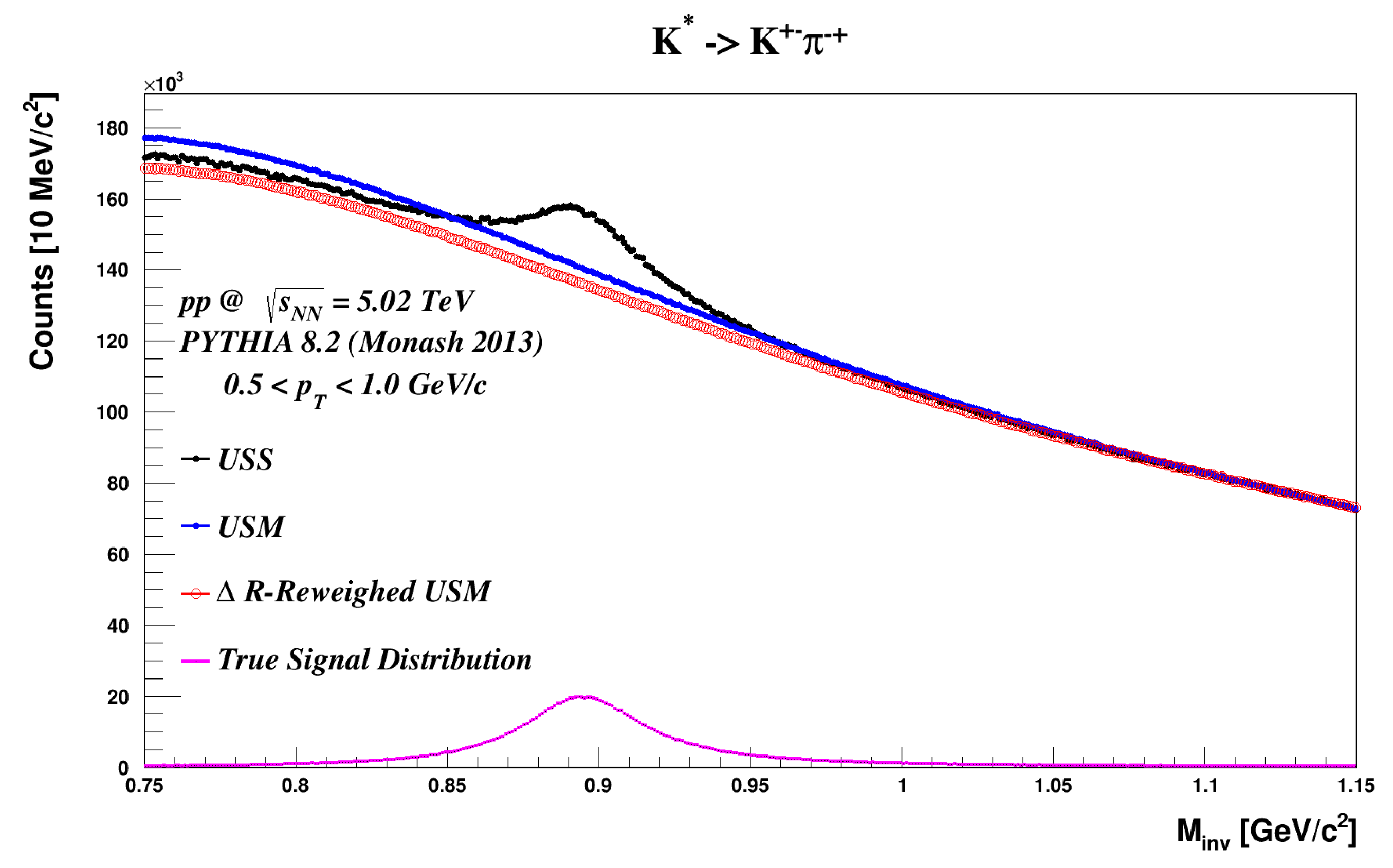
Figure 4 contains the resonance decay $K^{*}\to K^{+-}{\pi }^{-+}$ together with mixed-event distributions with and without $\Delta R$ reweighing. The background only consists of combinatorial pairs and pairs from non-K* sources. Both event-mixed backgrounds are normalized to the signal distribution at M${}_{inv}$ = 1.1–1.15 GeV/c${}^2$. The reduced signal-background spectra for the two different backgrounds are shown in Figure 5.

Figure 4 and Figure 5 highlight that, for simulated particle collisions in PYTHIA, normal event mixing is not able to accurately describe the combinatorial background seen in the M${}_{inv}$ distribution for K*(892) resonance decay, much like in real data. Applying a simple correction in respect to $\Delta R$, a measurement that only takes into account the $\Delta \varphi$ and $\Delta \eta$ between two particle tracks, has a very clear impact on the shape for the mixed-event background estimation. The impact of the $\Delta R$ correction varies for different M${}_{inv}$ and $p_{\mathrm{T}}$ intervals.

4. Conclusions

Although it is clear that there is a difference in topology between mixed-events and same-events (displayed in Figure 3), and that correcting for the difference in topology gives a more accurate estimation of the combinatorial background in the signal distribution (as observed in Figure 4 and Figure 5), it is not yet clear exactly how this correction should be performed. While $\Delta R$ re-weighing offers a very simple solution that outperforms a non-reweighed event-mixed distribution, one can note that the reweighed estimation in Figure 5 does not fully describe the combinatorial background. Adding a more complex correction scheme (taking into account both $p_{\mathrm{T}}$ and $\Delta R$) could improve the accuracy of the event-mixed background estimation, at the cost of increased complexity.