Abstract
Position location estimation in sensor networks is a valuable supplement since it supports the deployment of location-based services. Sensor networks have changing conditions in the environment due to propagation issues, noise and placement of sensors, which represent challenges that position location algorithms must deal with. Accuracy of the location estimation technique is relevant since it allows minimizing positioning error. In indoor environments, propagation issues such as multipath signals, affect adversely the precision of the positioning algorithm. Also, the use of parameters such as time of arrival has a trade-off between the small distances that the signals traverse and the precision of the hardware used to capture such measurements. In this paper, we use received signal strength indicator (RSSI) to estimate the coordinates of individual sensors in an area of study. The RSSI parameter is measured and processed by a set of reference nodes installed in the area. We show that performance of the location estimation algorithm needs additional techniques to obtain improved accuracy rate. We develop additional techniques based on the use of polynomial interpolation and spline functions to balance propagation issues. These techniques help us to implement correcting factors that are used in the propagation model to compensate the RSSI measurements. We use these techniques to show how the positioning error is reduced in the area of study with simulations and measurements using sensors.
1. Introduction
Localization is a task required for activities that need to know the precise (or at least an estimation of) position or location of some object or person; activities like tracking and monitoring of mobile robots for Simultaneous Localization And Mapping (SLAM) and localization of patients or staff in a building, to mention some of them [1,2,3,4]. Some tasks are harder to achieve than others, since some of them require a room-level accuracy and others require a high accuracy (typically in the order of few centimeters). The level or magnitude of the accuracy is mainly due to the technology being used for the localization process, and a more accurate system implies commonly, an expensive system. That is the case of Vision Based Localization Systems vs. Radio Frequency Based Localization Systems, where the first type of systems, could cost thousands of dollars, and the second type of systems, could cost tens of dollars. Nevertheless, the first kind of systems could have an accuracy of decimeters, while the second kind has typically an accuracy of meters [4,5].
Indoor Localization differs from Outdoor Localization in its complexity. While a systems like Global Navigation Satellite Systems (GNSS), from which Global Positioning System (GPS) is part of them, are preferred for Outdoor Localization, for Indoor Localization there are a lot of technologies and techniques that could be implemented; technologies based on mechanical systems, RF systems or vision systems, to name a few; and those techniques could rely on one or more physical measurements, like: Power of the Received Signal, Time of Flight of the Signal, Angle in which the Signal arrives, among others. Also, the system complexity can vary from one technology to other; the use of a lot of sensors could also increment the system’s complexity. For this work, RF based systems and RSSI technique was selected, since this kind of technologies are nowadays cheaper than others, are widely used and the RSSI technique is the most basic technique that one could use with this kind of systems, and finally, a total of 4 transceivers (sensors) were used, [6].
The challenging problem of indoor localization is due to the signal propagation behavior, because propagation effects are generally reliant on the particular area of study. In general, it is not possible to have models that make appropriate predictions of received power strength due to the different random components that are added to the signal. Among the different parameters used to perform localization, received power strength is the most problematic due to the random variations of the channel, specially for indoor environments, [7]. In previous work, [8], a locating algorithm was implemented measuring the received signal strength and calculating the root mean squared error of the difference of the actual position and the estimated by the algorithm. Once the environment was characterized in terms of path loss exponent and log-normal random variable, distance estimations were calculated by the direct use of the propagation model, and by maximum likelihood estimation. Also, in [8], to minimize the propagation effects due to multipath conditions, a correction factor was used by empirical analysis of sets of measurements of received signal strength, and the distance estimations between the point of interest and references were calculated using polynomial interpolations adjusting for optimal results on certain areas of the indoor environment.
2. Position Location Method
To improve the results of positioning, different methods have been proposed as possible solutions to improve the interpolation of [8] using the correction factor propagation model. The following methods have been considered: Adaptive Filters, [9], Interpolation using spline functions, [10], Method of Hilbert transformations, channel modeling. In this paper, we show the localization model, the polynomial interpolation method, polynomial interpolation with correcting factor and spline interpolation. To enhance localization, instead of polynomial interpolation, spline interpolation was used by adding information processing within the algorithm already established to improve the measurement results and consequently decrease the error position estimation method.
2.1. Experiment Setting
In [8], an environment is modeled to measure position using four antennas. Measurements and mathematical calculations of propagation models were performed to characterize the environment through the calculation of the path loss exponent and the standard deviation of the log-normal random variable for fadings. This is fed to algorithms that combine Euclidean distance equations between the antennas and the node of interest to obtain positioning results. The set of measurements obtained on site help empirically to determine a compensating factor which reduces the error caused by poor propagation prediction model and gives a more accurate result of the position.
The tested area as shown in Figure 1 shows the four antennas that were placed at a height of 2.3 m, the figure also shows how the experiment would take place evaluating the node position which is closest to the room floor. The coordinates of the reference antennas are identified in three dimensions, the separations of those antennas to the node provide the distance of interest. The results are then mapped to a two-dimensional coordinate system space to calculate the error.
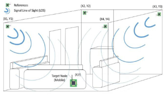
Figure 1.
Experiment environment.
2.2. The Location Problem
The location problem mainly consists of three stages as shown in Figure 2.
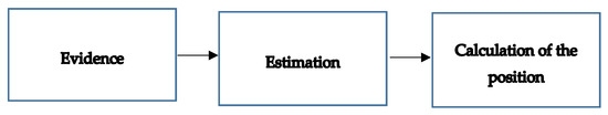
Figure 2.
The position location problem.
A brief description of each step is as follows:
- Evidence: It is the stage where measurements are made, received power evaluations (dBm) signals of the four reference antennas at different points of space are obtained.
- Estimation: it is the stage where the distance from the node of interest is calculated for each reference antenna using the propagation model and maximum likelihood criterion.
- Calculation of position: It is the stage where a system of equations based on estimated distances and Euclidean distances is generated and combined to calculate the estimated position of the node of interest.
3. Results
The traditional location model which is based on the classic triangulation works by measuring the strength of signals obtained from the antennae and the process of obtaining the distances which are the most reliable measurements to estimate location. These measurements and short distances are fixed and are used for calculating other distances. The transmission power is denoted as P0 and propagation models are modified according to this value to calculate received power at a distance d as in .
Figure 3 shows the stage where the received power is used for calculating distances to the node of interest from references, and that distance is drawn by a circle from each reference. These circles are combined through the system of equations is solved in the third stage of location problem.
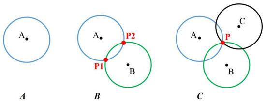
Figure 3.
Traditional position location by trilateration.
Spline Interpolation
The cubic spline interpolation is acknowledged by its handling of high-level polynomials to interpolate a function and smooth the values obtained in the section of evidence. We can calculate the position with this additional method. Once a set of reliable measurements of received signal strength are available, spline interpolation is used to represent estimated distances from the node of interest to the four references as a function of received signal strength. Thus, when the node of interest obtains a measurement of received signal strength, it uses splines to interpolate on the surface of distances to the references. In [8], polynomial interpolation was used.
The algorithm is trained using the set of measurements with which data of empirically estimated compensation factors and separation distances are set. The node of interest is placed in a certain position and the known reference transmit antennas are commanded to transmit a signal to the node of interest. The power of the signal transmitted by each of the reference antenna is received by the node of interest and its power is measured in dBm. With this information, interpolation is applied to the received power measurements node of interest to interpolate the separation distance according to the data set system that was trained.
Position error is obtained when no compensation factor, these results are shown in Figure 4.
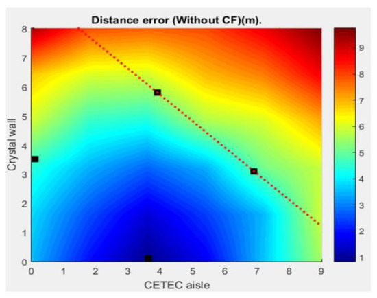
Figure 4.
Results without compensation factor.
The results of the Figure 4 show location errors of up to 10 m in the corners of the space of interest, due to the misbehavior of propagation model with random factors, and those need to be compensated to improve this error.
Figure 5 shows the same stages but now using compensation factor in the propagation model empirically estimated in the training system as described previously.
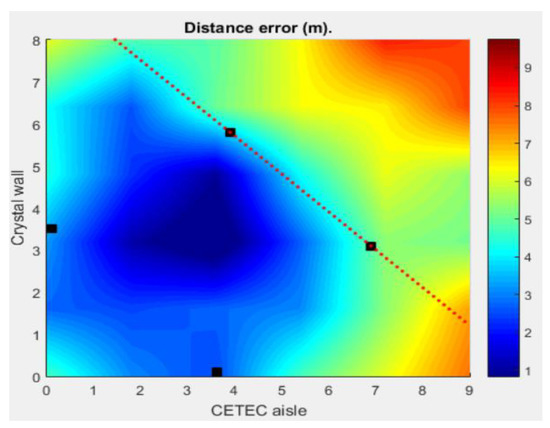
Figure 5.
Results with the use of compensation factor and polynomial interpolation.
Figure 5 compared to Figure 4 demonstrates that the location error is improved, now having better error performance around the area of interest, which is the lower triangle in the figures.
Figure 6 shows the use of spline interpolation and you can see a small growth of the blue area in the triangle of interest, hence improving error performance in that area.
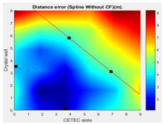
Figure 6.
Results using compensation factor and spline interpolation.
4. Discussion
Future direction for this research are the following: Implementation of a Wiener filter performing smoothing operation and substituting the spline functions. Correction coefficients for Splines, the use of Hilbert transform to smooth spectrally the propagation measurements, channel modeling by using measurements of power delay profile.
5. Conclusions
In conclusion, the implementation of spline interpolation generates the values of the interpolated distances using fewer resources and avoiding an increased degree of the polynomial hence having a better efficiency of resources to process the data obtained. In the results presented the method of spline interpolation is used as an additional method, and it is effective for the results of the location of the position and its results are better than to those presented without compensation factor and with compensation factor.
Author Contributions
Alvaro Alonso Garcia-Davila was in charge of the spline interpolation, Erasmo Ortega performed the measurements and characterization of the environment. Cesar Vargas-Rosales conducted the correcting factor and polynomial interpolation techniques, and Jose Luis Gordillo established the experiment scenario at the Robotics laboratory.
Acknowledgments
This work was partially supported by the Research Focus Groups of Telecommunications and Networks and the group of Robotics at Tecnologico de Monterrey.
Conflicts of Interest
“The authors declare no conflict of interest." “The founding sponsors had no role in the design of the study; in the collection, analyses, or interpretation of data; in the writing of the manuscript, and in the decision to publish the results”.
References
- Artemenko, O.; Schorcht, G.; Tarasov, M. A refinement scheme for location estimation process in indoor wireless sensor networks. In Proceedings of the IEEE GLOBECOM Workshops (GC Wkshps), Miami, FL, USA, 6–10 December 2010; pp. 225–229. [Google Scholar]
- Miraoui, A.; Mabrouk, K.; Snoussi, H.; Amerhaye, A.; Duchene, J. A large scale and low cost solution for real-time indoor localisation based on wireless sensor network. In Proceedings of the 7th International Workshop on Systems, Signal Processing and their Applications (WOSSPA), Tipaza, Algeria, 9–11 May 2011; pp. 392–395. [Google Scholar]
- Kuai, X.; Yang, K.; Fu, S.; Zheng, R.; Yang, G. Simultaneous localization and mapping (slam) for indoor autonomous mobile robot navigation in wireless sensor networks. In Proceedings of the 2010 International Conference on Networking, Sensing and Control (ICNSC), Chicago, IL, USA, 10–12 April 2010; pp. 128–132. [Google Scholar]
- Elnahrawy, E.; Li, X.; Martin, R. The limits of localization using signal strength: a comparative study. In Proceedings of the 2004 First Annual IEEE Communications Society Conference on Sensor and Ad Hoc Communications and Networks (IEEE SECON 2004), Santa Clara, CA, USA, 4–7 October 2004; pp. 406–414. [Google Scholar]
- Mautz, R. Indoor Positioning Technologies. Ph.D. Dissertation, ETH Zurich, Zurich, Switzerland, 2012. [Google Scholar]
- Yang, Z.; Zhou, Z.; Liu, Y. From RSSI to CSI: Indoor localization via channel response. ACM Comput. Surv. 2004, 46, 1–33. [Google Scholar] [CrossRef]
- Muñoz, D.; Bouchereau, F.; Vargas, C.; Enriquez-Caldera, R. Position Location Techniques and Applications, 1st ed.; Academic Press/Elsevier: Amsterdam, The Netherlands, 2009. [Google Scholar]
- Chavarria, E.O. Design and Implementation of a Radio Frequency for Indoor Localization. Master's Thesis, Instituto Tecnologico y de Estudios Superiores de Monterrey, Monterrey, NL, Mexico, December 2015. [Google Scholar]
- Haykin, S.S. Adaptive Filter Theory, 4th ed.; Prentice Hall: Upper Saddle River, NJ, USA, 2014. [Google Scholar]
- C. de, Boor. A Practical Guide to Splines; Springer-Verlag: New York, NY, USA, 1978. [Google Scholar]
Publisher’s Note: MDPI stays neutral with regard to jurisdictional claims in published maps and institutional affiliations. |
© 2016 by the authors. Licensee MDPI, Basel, Switzerland. This article is an open access article distributed under the terms and conditions of the Creative Commons Attribution (CC BY) license (https://creativecommons.org/licenses/by/4.0/).