Abstract
In wireless sensor networks (WSN) localization of the nodes is relevant, especially for the task of identification of events that occur in the environment being monitored. Thus, positioning of the sensors is essential to satisfy such task. In WSN, sensors use techniques for self-localization based on some reference or anchor nodes (AN) that know their own position in advance. These ANs are fusion centers or nodes with more processing power. Assuming that the number of ANs given in the network is N, we carry out the localization algorithm to position sensors sequentially using those N ANs. Now, when a sensor has been localized, it becomes a new AN, and now, other sensors will use N + 1 ANs, this is repeated until all the sensors in the network have been localized. In this sequential localization algorithm, the positioning error (difference between true and estimated position) increases as the sensor to be located is farther away from the group of original ANs in the network. This error becomes critical when propagation issues such as multipath propagation and shadowing in indoor environments are considered. In this paper, we characterize statistically positioning error in WSN for one-dimensional indoor environments when sensors are deployed randomly. We also evaluate the performance of the localization algorithm and determine correcting factors based on the statistical characterization to minimize positioning error. We present results from simulations and measurements in an indoor environment.
1. Introduction
In 1996, the FCC made a statement requesting phone service providers to have a way to reach their customers for reasons of safety (a more efficient service to emergency calls) [1]. This requirement has evolved and the position location techniques being proposed have intensified, and various services related to this technology have emerged, such as new forms of advertising, payments and sales services [2]. There is already a localization method based on satellites, the Global Positioning System (GPS), that still presents difficulties, such as the lack of precision in relatively closed environments, and we must also consider the implications of the use of devices with GPS that carry a higher-cost of the products, larger dimensions and more energy being spent [1]. This contrasts with the proposal of developing a technique that uses existing or easy to install infrastructure, as well as a wireless device without additional sensors. This is why, it is important to develop an algorithm that uses efficiently the existing conditions in the wireless environment that allows the localization in a sensor network of the nodes scattered randomly using as parameter the Received Signal Strength or RSS [1].
Traditional localization techniques are based on the measurement of a parameter such as RSS, time of arrival (TOA), time difference of arrival (TDOA) or angle of arrival (AOA) and the combination of distance estimation in a trilateration or multilateration process [3]. In wireless ad-hoc and sensor networks, there have been different algorithms in the literature that apply relational techniques in combination with distance estimation through RSS or time of arrival (TOA), e.g., see [4,5,6], some of those techniques use a reference grid [6], and distances are estimated in terms of hops in the routes connecting ANs and nodes of interest. Also, these ideas have been extended to consider three-dimensional scenarios, see [7].
In this paper, we introduce a position location technique based on RSS measurements and classical propagation models to estimate distance and combine references to obtain position of sensor nodes in a network. The estimation is verified by reference nodes in several instances to balance the propagation effects of multiple paths in indoor environments. Location is obtained by averaging the positioning of those instances executed in the algorithm.
2. Position Location Algorithm
The localization algorithm that we propose, works under the theoretical foundation that it establishes that the received power or RSS is directly proportional to the transmission power and inversely proportional to the distance between receiver and transmitter with a path loss exponent (PLE) that was obtained experimentally by measuring in an indoor environment. PLE was obtained by averaging, by using linear regressions, and by using maximum likelihood techniques with the RSS measurements. We consider the scenario where sensors are scattered in a one dimensional arrangement, the network has a known amount of reference nodes or anchor nodes (AN). These ANs have fixed and known positions in the network. Also, the position of one of the ANs is known by all the other ANs. There is a maximum distance covered by the one dimensional arrangement. It is necessary to mention that two of the reference nodes are located at the origin and at the end of our one dimensional scenario, respectively.
ANs partition the one dimensional scenario in adjacent and non-overlapping segments, where the first segment corresponds to those ANs n1 and n2, and the last segment is formed by reference nodes nN-1 and nN. Reference node k or k-th AN is denoted by nk, and N is the total number of reference nodes in the network. The algorithm is executed in several stages. In each stage it performs three tasks for every node to be located:
- Data acquisition: RSS is measured in a real environment, i.e., any measurement will be considered to come from a propagation model with PLE known and a standard deviation of a log-normal random variable
- Data interpretation: RSS is used to estimate separation distance between the reference node and the node to be located.
- Data combination: With distance estimations, combine them with a system of equations in order to obtain coordinates of node to be located.
After the three tasks have been performed and given the definition of segments by the reference nodes, ANs will then proceed to the First classification of data. This first classification is given by the distance estimated by AN at the origin, i.e., n1, of all the nodes to be located at the network. This first classification has the purpose of assigning a segment to each node to be located. Later a refinement algorithm will be used to actually estimate position of the nodes, but first ANs only want to define the segment where nodes to be located are. A vector contains the absolute value of the differences between the true distance and the distances calculated of the nodes to the reference. The smallest difference is chosen to determine the reference node that is next to the node to be located.
Next, a second classification is performed. Intermediate ANs are considered in order to determine the segment where nodes to be located are. If a node to be located was misplaced in an adjacent segment instead of its actual segment, this procedure will try to “take it back” to the place it is supposed to be. Intermediate reference nodes will see if such node to be located belongs to its left or right depending on RSS measurements and comparison to RSS measurements with other ANs. This is performed several times (at least three) where measurements of RSS are obtained in each time, and estimations are averaged.
After the second classification, a third classification is performed, which is essentially the same as the first classification, but the starting reference node instead of being AN n1, is now AN nN. There is a verification stage that is carried out after the third classification to deal with estimations that could fall out of the scenario or to place nodes that have been misplaced.
3. Results
For the results, the experiments where conducted in different scenarios where the number of ANs was varied and the length of the one dimensional network was also increased. Mean squared error of the distance between the estimated position and the true position was obtained. Since for each node to be located, we have several readings of estimated positions coming from all the different ANs, these estimations were averaged arithmetically. For each RSS measurement, a log-normal random variable with zero mean and standard deviation of 8 dB was considered, generating uncorrelated random variables of power received from a node to be located at different ANs. The scenarios for the results varied the number of nodes to be located, the number of reference nodes, the length of the one dimensional network, and keeping all parameters fixed.
Since our main objective is to present the statistical characterization of the localization error, we present the probability density function (pdf) estimation for the scenarios analyzed. In all experiments we fixed information such as the nodes to be located that is 20 and in some scenarios is varied from 2 up to 100, the number of ANs is 10 and the scenario has a length of 100m.
Figure 1a shows the probability density function estimated of the mean squared error for the scenario when the number of nodes to be located is kept constant. On the other hand, Figure 1b shows the same scenario but when the nodes to be located are varied from 2 up to 100. As we can see in these two figures, the density function does not change significantly, meaning that the algorithm is not affected by the increase in nodes to be located. The mean value, i.e., the peak of the functions is practically the same, and the standard deviation is bigger just a little in the second scenario. Also, when nodes to be located are varied, the density function has more symmetry around the mean value than that of the scenario when nodes to be located are fixed. These two scenarios show that mean squared error is more dependent on the number of references than the number of nodes to be located.
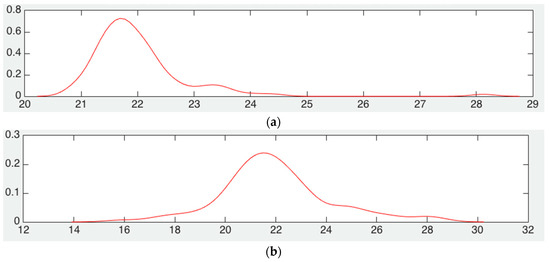
Figure 1.
Estimation of MSE pdf with fixed reference nodes, (a) number of nodes to locate is constant, (b) number of nodes to locate varies from 2 to 100.
In Figure 2a, we show the scenario where the number of nodes to be located is fixed to 20, and then the 10 reference nodes are fixed in certain positions and the simulation is performed several times to estimate density. In Figure 2b we have the scenario under the same conditions as those just mentioned, but the 10 reference node positions are changed randomly in the network and mean squared error is calculated. From the figures, we can conclude that the error is basically the same for both scenarios, and once again the difference is given by the standard deviation of each of these scenarios, where the scenario with randomly placed reference nodes has a larger value of standard deviation that the one in Figure 2a.
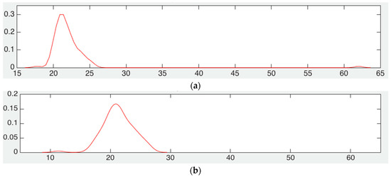
Figure 2.
Estimation of MSE pdf with randomly placed reference nodes, (a) number of nodes to locate is constant, (b) number of nodes to locate varies from 2 to 100.
Now if we fix the number of reference nodes at 10, we fix the length to 100 m, and then vary the number of nodes to be located from 2 up to 100, we have results in Figure 3. We show the 100 mean squared error data obtained from 100 simulations in the dots in Figure 3a,b. Also those figures have a red line that indicates the cumulative probability distribution function. For example, in Figure 3a you can see that the red line indicates that 90% of the time (horizontal axis) the error will be of 24 or less meters (vertical axis). Figure 3b has a similar result but when the number of reference nodes is placed randomly in the network. We can also appreciate that basically both figures have essentially the same cumulative distribution function.
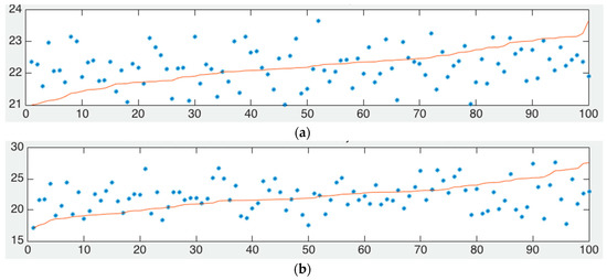
Figure 3.
Data points and cumulative distribution function for scenario where nodes to be located are varied from 2 up to 100, (a) fixed position of reference nodes, (b) random position of reference nodes.
Figure 4a,b show the probability density function estimated for the scenario shown in Figure 3a,b, respectively.
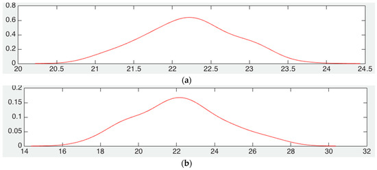
Figure 4.
Estimation of MSE pdf with fixed reference nodes, (a) fixed position of reference nodes, (b) random position of reference nodes.
In Figure 4a we can see the probability density function of the scenario of Figure 3a,b when reference nodes are at fixed positions. Figure 4b have the results when the reference nodes are placed randomly at every time simulation is executed, under the same conditions. We can see that what changes mostly is the standard deviation, being larger in value when reference nodes are randomly placed.
4. Conclusions
The mean squared error for localization has been obtained for a one-dimensional scenario. Even if conditions such as number of nodes to be located, fixed or random positons of reference nodes and length of network are changed, we can see that mean squared error remains with the same mean value, and what changes is the standard deviation especially when the reference nodes are placed randomly. So, the application to a real scenario would be better if reference nodes are fixed at known positions to have less variance of error.
Acknowledgments
This work was partially supported by the Research Focus Groups of Telecommunications and Networks and the group of Robotics at Tecnologico de Monterrey.
Author Contributions
Cesar Vargas-Rosales carried out the writing of the paper and the main idea behind the location algorithm to consider propagation models. Yasuo Maidana programmed the whole algorithm and organized its execution in the three classification stages described. Rafaela Villalpando-Hernandez and Leyre Azpilicueta were in charge of the field measurements of received signal strength where path loss exponent and variance of signal propagation were calculated using maximum likelihood, averages and inverse propagation models.
Conflicts of Interest
The authors declare no conflict of interest. The founding sponsors had no role in the design of the study; in the collection, analyses, or interpretation of data; in the writing of the manuscript, and in the decision to publish the results.
References
- Sayed, A.H.; Tarighat, A.; Khajehnouri, N. Network-based wireless location: challenges faced in developing techniques for accurate wireless location information. IEEE Signal Process. Mag. 2005, 22, 24–40. [Google Scholar] [CrossRef]
- Gunnarsson, F.G.Y.F. Mobile positioning using wireless networks: possibilities and fundamental limitations based on available wireless network measurements. IEEE Signal Process. Mag. 2005, 22, 41–53. [Google Scholar]
- Munoz, D.; Bouchereau, F.; Vargas, C.; Enriquez, R. Position Location Techniques and Applications, 1st ed.; Academic Press/Elsevier: Amsterdam, The Netherlands, 2009. [Google Scholar]
- Perez-Gonzalez, V.; Munoz-Rodriguez, D.; Vargas-Rosales, C.; Torres-Villegas, R. Relational Position Location in Ad-Hoc Networks. Ad-Hoc Netw. 2015, 24, 20–28. [Google Scholar] [CrossRef]
- Vargas-Rosales, C.; Mass-Sanchez, J.; Ruiz-Ibarra, E.; Torres-Roman, D.; Espinoza-Ruiz, A. Performance Evaluation of Localization Algorithms for WSNs. Int. J. Distrib. Sens. Netw. 2015, 2015, 493930. [Google Scholar] [CrossRef]
- Villalpando, R.; Munoz-Rodríguez, D.; Vargas-Rosales, C.; Rodríguez, J.R. Position Location in Ad-hoc/Sensor Networks: A Linear Constrained Search. IEEE Commun. Lett. 2011, 15, 605–607. [Google Scholar] [CrossRef]
- Villalpando-Hernandez, R.; Muñoz-Rodriguez, D.; Vargas-Rosales, C.; Rizo, L. 3-D Position Location in Ad-hoc Networks: A Manhattanized Space. IEEE Commun. Lett. 2016, 21, 124–127. [Google Scholar] [CrossRef]
Publisher’s Note: MDPI stays neutral with regard to jurisdictional claims in published maps and institutional affiliations. |
© 2016 by the authors. Licensee MDPI, Basel, Switzerland. This article is an open access article distributed under the terms and conditions of the Creative Commons Attribution (CC BY) license (https://creativecommons.org/licenses/by/4.0/).