Article

Bootstrapping Enhanced Model for Improving Soil Nitrogen Prediction Accuracy in Arid Wheat Fields

by
Qassim A. Talib Al-Shujairy
1,
Suhad M. Al-Hedny
1,*,
Mohammed A. Naser
2,
Sadeq Muneer Shawkat
3,
Ahmed Hatem Ali
1 and
Dinesh Panday
4,*
1
College of Environmental Sciences, Al-Qasim Green University, Babil 51013, Iraq
2
Department of Combating Desertification, College of Agriculture, Al-Muthanna University, Al-Samawah 66001, Iraq
3
College of Food Sciences, Al-Qasim Green University, Babil 51013, Iraq
4
Rodale Institute, Kutztown, PA 19530, USA
*
Authors to whom correspondence should be addressed.
Nitrogen 2025, 6(2), 23; https://doi.org/10.3390/nitrogen6020023
Submission received: 31 January 2025 / Revised: 25 March 2025 / Accepted: 26 March 2025 / Published: 1 April 2025

Abstract

:
Soil nitrogen (N) is a crucial nutrient for agricultural productivity and ecosystem health. The accurate and timely assessment of total soil N is essential for evaluating soil health. This study aimed to determine the impact of bootstrapping techniques on improving the predictive accuracy of indirect total soil N in conventional wheat fields in Al-Muthanna, Iraq. We integrated a novel methodological framework that integrated bootstrapped and non-bootstrapped total soil N data from 110 soil samples along with Landsat 9 imagery on the Google Earth Engine (GEE) platform. The performance of the proposed bootstrapping-enhanced random forest (RF) model was compared to standard RF models for soil N prediction, and outlier samples were analyzed to assess the impact of soil conditions on model performance. Principal components analysis (PCA) identified the key spectral reflectance properties that contribute to the variation in soil N. The PCA results highlighted NIR (band 5) and SWIR2 (band 7) as the primary contributors, explaining over 91.3% of the variation in soil N within the study area. Among the developed models, the log (B5/B7) model performed best in capturing soil N (R2 = 0.773), followed by the ratio (B5/B7) model (R2 = 0.489), while the inverse log transformation (1/log (B5/B7), R2 = 0.191) exhibited the lowest performance. Bootstrapped RF models surpassed non-bootstrapped random forest models, demonstrating enhanced predictive capability for soil N. This study established an efficient framework for improving predictive capacity in areas characterized by limited, low-quality, and incomplete spatial data, offering valuable insights for sustainable nitrogen management in arid regions dominated by monoculture systems.

1. Introduction

The application of fertilizer inputs, particularly nitrogen (N), is essential for maintaining soil health in high yield cropping systems [1]. On a global scale, only half of the N fertilizer applied is retrieved by harvested crops, while the rest is susceptible to environmental losses via volatilization, leaching, and/or emissions [2]. These losses significantly affect air and water quality, leading to issues such as surface water eutrophication and groundwater contamination [3]. Conversely, the inadequate application of N fertilizers leads to poor crop growth and reduced yields. Therefore, determining the optimal N application across entire fields has become increasingly critical [4,5].
The traditional method for determining the optimal N rate recommendation relies entirely on the crop’s demand and the available soil N supply. However, this approach does not account for the significant variability in the optimal soil N rates observed from one field to another. The spatial differences in both crop N demand and soil N supply underscore the need to improve our understanding of where and how much N should be applied [6]. A field-based assessment of soil N distribution offers a highly accurate way to optimize N fertilizer applications; however, this approach is time-consuming and costly, requiring a dense network of sampled points.
To overcome these limitations, remote sensing techniques present an effective alternative to traditional laboratory analysis methods. Numerous studies have underscored the potential of soil spectral reflectance and regression modeling for mapping soil properties under various environmental conditions worldwide [7,8,9]. Research has examined the feasibility of using spectral reflectance, particularly near-infrared spectroscopy, to quantify soil N content, as well as the factors influencing the determination model [10,11,12]. A strong predictive capability of soil N, with an R2 value of 0.84 between laboratory-measured and predicted total N values, was achieved through the application of proximal sensing methods in wheat fields across two arid-region sites [13]. Despite this progress, the limited availability of field data poses a significant challenge for estimating soil properties using remote sensing approaches. This challenge is particularly evident in arid agricultural areas, where soil properties can change markedly at small field scales.
Machine learning models, especially the random forest (RF) algorithm, have proven effective in capturing complex and nonlinear interactions between soil properties and spectral data. Random forest has been widely employed to estimate spatial variations in soil properties [14,15,16]. Although machine learning algorithms often yield improved predictions of soil N, their accuracy is influenced by several factors, including land use, management practices, crop type, soil type, and environmental conditions [17,18]. To mitigate common challenges in predicting soil properties, researchers have explored various approaches, such as identifying optimal wavelength combinations [19], downscaling multiscale geospatial data [20], and employing multiple algorithms within a land parcel-based framework, to enhance the accuracy of soil nutrient predictions in agricultural plains [21].
Additionally, statistical techniques were applied to create new datasets from an existing sample dataset using a bootstrapping approach [22], which provided justifiable results and minimized errors in modeling. As an effective statistical technique, bootstrapping is increasingly favored for evaluating statistically significant trends using real-world data [23,24]. There are two primary types of bootstrapping procedures: nonparametric and parametric. Nonparametric resampling techniques utilize the data and are often employed with smaller datasets, while parametric methods assume a predefined distribution and use estimated parameters or statistics to generate new datasets [25].
Bootstrapping offers soil engineers the ability to predict design parameters based on randomly measured properties of interest. For instance, ref. [26] utilized bootstrapped soil datasets to estimate the vertical variation of the soil cone index, demonstrating the effectiveness of bootstrapping in estimating soil resistance under varying management practices. The study in [27] achieved more accurate analyses and precise estimations in soil texture prediction models developed using a single bootstrap Geographically Weighted Regression (GWR)-based method. Previous studies primarily concentrated on generating a large sample from originally small soil datasets to reduce uncertainty and promote convergence in soil property variations [28,29,30,31].
The current study introduces a bootstrapping-enhanced RF model by applying a layer of nonparametric bootstrapping to improve model robustness and assess uncertainty in soil N predictions under conditions of limited data availability. Unlike conventional RF models, which resample only at the tree level, this approach incorporates additional iterations at the original dataset level, ensuring a more comprehensive training process.
The integration of remote sensing with Google Earth Engine (GEE) further enhances soil monitoring by providing immediate access to a vast catalog of historical high-resolution satellite imagery and global datasets. GEE enhances data processing capabilities, providing an efficient framework for large-scale analysis and serving as a valuable tool for addressing sustainable development challenges. By leveraging processing power, GEE supports a variety of machine learning algorithms, including partial least squares regression (PLSR), Bayesian regularized neural networks (BPNN), support vector machines (SVM), and RF [32,33] to create soil-specific models.
In this study, a customized bootstrap-based RF approach was integrated with remote sensing to improve total soil N prediction modeling, addressing national requirements for rapid monitoring responses. The objectives were to (i) develop and assess a remote sensing-based framework for predicting soil N in data-scarce regions, (ii) assess the impact of customized bootstrap-based RF modeling strategy, and (iii) emphasize the importance of remote sensing in enhancing soil fertility management.

2. Materials and Methods

2.1. Study Area and Soil Sampling

The study area is situated in the Al-Rumeytha district of the Al-Muthanna governorate in southern Iraq. Al-Muthanna covers 12% of Iraq’s total area and is defined by latitude and longitude coordinates of 31.3132184° and 45.2845512°, respectively. Spanning an area of 51,740 km2, the Al-Muthanna governorate is divided into four districts: Al-Samawa (the capital), Al-Rumaitha, Al-Khidhir, and Al-Salman. The region experiences a desert climate characterized by an average annual rainfall of 89.5 mm, with summer temperatures reaching as high as 50 °C. The soil in this area is predominantly sandy and silty, resulting in low water-holding capacity. The Euphrates River serves as the primary source of irrigation for the study area, which is predominantly used for wheat cultivation.
A handheld Garmin eTrex Global Position System (GPS) was used to record the latitude and longitude data of 110 soil samples. We collected soil samples in November 2023 at a sampling depth of 0–20 cm (Table 1). All sampled soils were air dried, then the gravel and plant residuals were picked out, and, after gridding, were sieved to 2 mm. Soil samples were conventionally analyzed for the total soil N by the Kjeldahl method [34]. A total of 70% of the observations from the total observations (n = 110) from each cropping system was randomly selected to construct the training set (n = 77), and the remaining 30% was used for testing (n = 33).

2.2. Image Capture and Processing

Landsat imagery from November 2023 was obtained via the GEE platform. In January 2024, seamless access to Landsat 9 imagery data was available through this cloud-based resource (https://earthengine.google.com). This study focused on the highest geometric accuracy Landsat 9 Surface Reflectance (SR) images found in the catalogue (LANDSAT/LC09/C02/T1_L2). The GEE provides Top of Atmosphere (TOA) images that have been converted to SR and reprocessed for radiometric corrections, cropping, and geometric adjustments. The use of SR image collections streamlines data processing and enhances the accuracy of soil N predictions.

2.3. Identifying Key Reflectance Bands

The acquired images were integrated with field-based data to filter the soil N characteristic bands, as outlined in Figure 1. Relating specific soil properties to soil spectra is a complex task; therefore, regression analysis is commonly employed to quantitatively link soil reflectance data to specific soil properties. Principal component analysis (PCA) was conducted on the Landsat 9 data to filter sensitive bands. The components identified through this analysis were utilized to pinpoint the bands most closely related to total soil N compared to others. PCA calculates the variance and mean of each input variable and the covariance (COV) between variables to create a covariance matrix. The COV is then transformed to yield independent components that are linear combinations of the original inputs. These uncorrelated components account for the maximum variance in the target value and can be utilized as inputs to the model [35].
The eigenvectors of the covariance matrix from the PCA analysis, which revealed high loading factors and variance, explained the percentage utilized to compute Pearson’s correlation coeffeicient (r) to verify their relationships with the soil N dataset. To investigate the relationships between soil N and reflective bands, the study incorporated derived spectral indices into Landsat 9 imagery for additional analysis. The Sample Region function in GEE was employed to extract index reflectance values at the soil sampling sites, enabling the calibration of the RF machine learning algorithm. Ultimately, the model’s accuracy for total soil N prediction was determined using performance metrics, specifically the root mean square error (RMSE) and the coefficient of determination (R2).

2.4. Model Selection and Validation

In the current study, the RF machine learning algorithm was utilized to predict soil N across the entire study area. The research concentrated on three derived indices to enhance the predictive capability of the RF model. The first input feature was the simple ratio of bands, followed by the logarithmic transformation of the band ratio and its inverse. A decision tree-based RF algorithm was employed to predict the spatial variation of soil N, where RF enhances the prediction model by reducing overfitting and effectively addressing abnormal data types.
To ensure the optimal performance of the RF algorithm, we manually specified several parameters: the number of trees (n-tree), the minimum size of the terminal node (node-size), the number of predictor variables (the spectral indices) in each node (m-try), and the maximum depth of the trees. In this study, we processed the RF algorithm using the GEE platform, setting the parameters to 100 for n-tree, 3 for m-try, and 5 for node-size, with a tree depth of 10. The number of trees was chosen to enhance model consistency, while m-try was manually adjusted to find the optimal value based on its correlation with soil N. Node size and tree depth were specified to balance prediction accuracy with computational efficiency. The RF algorithm calculates a weighted average of each calibrated value based on the training data. The Sample Region function in GEE randomly divided the soil sample dataset, allocating 70% for training and reserving the remaining 30% for model validation. Model performance was assessed using the R2 and RMSE as performance metrics. The prediction model that achieved the highest R2 and lowest RMSE was used to create a spatial map depicting total soil N variation across the study area.

2.5. Bootstrapping Implementation

To improve the predictive accuracy of soil N estimation using remote sensing, we implemented a tailored nonparametric bootstrapping method. This method generates multiple resampled datasets to mitigate site variation. The bootstrapping process was computed in Google Colab, where we used random replacement to generate 1000 resampled training datasets from the original soil dataset (B = 1000 # Number of bootstrap samples). This replacement prevents data leakage between the training and test sets to minimize site-specific variation within the study area by omitting some samples, while others may appear multiple times. This strategy was specifically crafted to provide a more representative distribution of soil N data, especially in the highly skewed conditions typical of arid regions. Furthermore, the study employed a reweighting to balance underrepresented and overrepresented N level and mitigate the impact of extreme values. A Dirichlet distribution was employed to apply non-uniform weighting to ensure that each resample obtained a different distribution of importance across observation, and it followed this python code:
boot_sample = train_df.sample (n = len(train_df), replace = True, weights = train_df[‘weights’], random_state = None)
Under the reweighting step, each sample may appear multiple times or not at all in boot_sample. We determined the number of times each sample appears in the resampled dataset, sample_counts = boot_sample.index.value_counts (normalize = True), which was normalized by total sample size as in the following python code:
boot_sample[‘normalized_frequency’] = boot_sample.index.map (sample_counts)
This process was repeated for a predefined number of bootstrap samples to address spatial heterogeneity throughout the study area. The tailoring approach allowed certain samples to have an influence on model training. This means that the samples prioritized by the model appear more times in the resampled dataset rather than treating all samples equally as in the uniform weighting approach.
To assess uncertainty in the model performance, a 95% confidence interval (CI) was utilized [36]. The standard deviation and mean prediction were used to compute the CI by using the following formula:
C I 95 % = y ^ ± 1.96 × σ b o o t s t r a p B
where B is the number of bootstrap iterations, y ^ is the mean prediction from all iterations, σ is the standard deviation across all bootstrap samples, 1.96 corresponds to the confidence level of 95% under a normal distribution assumption. This CI approach allowed the prediction model to consider the anticipated range of soil N values under real-field conditions. Additionally, noise filtering was applied through 1000 sampling iterations, which improved the stability and reliability of the tailored bootstrapping method [37,38].
The study methodology consists of two main phases: data preprocessing in GEE; specifically, the derived indices were exported as a dataset to Google Colab for further model implementation as a second phase of the applied methodology. In this environment, the RF model was trained on each resampled dataset individually. This approach ensured that the model accurately represented real-site variability instead of overfitting to a single dataset. Additionally, the performance of both the bootstrapped and non-bootstrapped RF models was validated, confirming the reliability of the soil sampling process across various field conditions.

3. Results and Discussion

3.1. Features Derivation

The average concentration of soil N across the studied cropland was measured at 725 ppm, with a coefficient of variation (CV) of 36.7%. PCA was utilized to identify the spectral bands most indicative of variations in soil N content. The eigenvalues derived from PCA quantified the amount of variance in the original variables assigned to each principal component, aiding in the selection of bands that were most correlated with soil N predictions (Table 2).
According to PCA findings, the near-infrared band (B5) demonstrated the highest loading factor in principal components PC1 (−0.58) and PC3 (0.72), while B7 contributed to PC1 (0.42), PC3 (0.38) and was strongly associated with PC2 (−0.82). The first PC explains the highest overall variation in spectral bands (25.12%) with a low Pearson correlation coefficient (r < 0.4), indicating that it maximized variance without considering the N variable in the dataset. Although PC2 and PC3 captured a lower variance of 20.84% and 21.71%, respectively, they had a high Pearson correlation coefficient (r > 0.8), suggesting better capture variation linked to soil N. Furthermore, to validate that the high loading factors of B5 and B7 are related to soil N contents, Pearson’s correlation was directly applied to both bands individually as well as for their averaging values. Collectively, bands 5 and 7 accounted for over 91.3% of the spatial variation soil N across the study area, revealing a strong Pearson correlation with soil N (r = 0.955).
These bands are indirectly related to soil N, wherein the positive correlation of band 5 with vegetation reflectance aligns well with findings from previous studies [39,40,41]. Meanwhile, the negative correlation with band 7 (SWIR2) suggests that higher reflectance is associated with lower soil N content. The selected crop field in the study area was characterized by low organic matter and moisture levels, which minimized confusion from signal overlapping with other soil properties, enhancing the effectiveness of these spectral bands as diagnostic tools under the specific conditions of this study.
The PCA findings clarified the intricate relationships between spectral bands and soil N content, facilitating the development of spectral indices. Furthermore, these findings underscored the significance of PCA in pinpointing the most influential bands and guiding input features to explain variations in soil N content [41].
Based on the PCA results, three spectral indices were formulated: the simple ratio of bands 5 and 7, expressed as (B5/B7); the logarithm of this band ratio log (B5/B7); and the inverse of the logarithmic transformation 1/log (B5/B7). These indices were chosen to substitute for the reflectance values of Landsat 9 bands in RF models. The integration of these indices within a cloud-based geospatial framework enabled the efficient processing of spectral reflectance data across the Al-Rumaitha district. This approach facilitated both PCA and RF algorithms in extracting key spectral features and evaluating various mathematical transformations under different prediction scenarios.

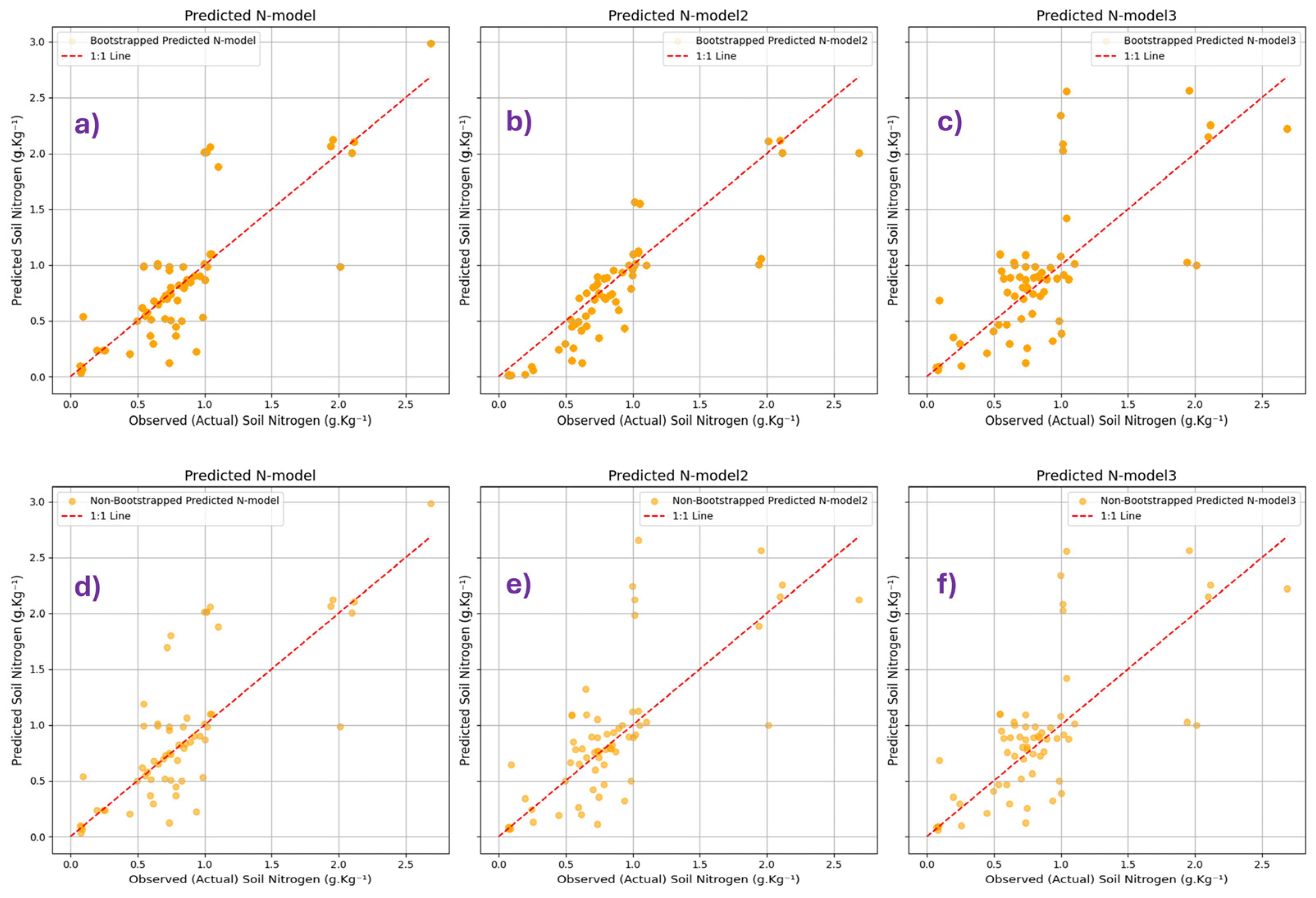
3.2. Bootstrapping vs. Non-Bootstrapping Models

Among the tested models, the log (B5/B7) model delivered superior results, explaining 61.49% of soil N variation with a non-bootstrapped RF, which increased to 77.3% (R2 = 0.773) when the bootstrapped RF was utilized (Table 3). The logarithmic transformation of band ratios reduced unintended interactions in spectral reflectance and minimized the impact of noisy data, while enhancing the differences in soil reflectance values.
Bootstrapping effectively mitigated data variability and corrected the bias caused by the non-uniform distribution of total soil N. The simple ratio (B5/B7) model demonstrated moderate predictive ability with an R2 of 0.489 under bootstrapped conditions, but it struggled to capture soil N variability effectively (Table 3). The predictive capability of the inverse logarithmic model (1/log (B5/B7)) was the lowest throughout all assessments due to its inability to accurately represent variability in soil reflectance. Notably, both bootstrapped and non-bootstrapped RF models provided nearly identical mean predictions since they relied on the same total soil N dataset.
The overall enhancement in model performance through bootstrapping was further supported by improved RMSE values. The log (B5/B7) displayed a slight reduction in RMSE under bootstrapping, decreasing from 0.17 to 0.10. This indicates that the bootstrapped model provided better precision in predicting total soil N levels. Additionally, the bootstrapped RF log (B5/B7) model showed a narrower confidence interval than other bootstrapped RF models, with a range of 0.723–1.026, suggesting that the true mean of the bootstrapped log B5/B7 RF model lies within positive and well-defined values. Such narrow intervals indicate greater confidence in the model’s performance and reveal a higher level of certainty. In contrast, both the ratio and inverse logarithmic ratio models presented wider confidence intervals. The bootstrapped RF ratio (B5/B7) model recorded a mean value of 0.85, which lies outside the confidence interval range of 0.074–0.216. This outcome reflects the model’s limited predictive capacity in handling the inherent variability of the data. The confidence interval is derived based on the range where most of the predictions lie, but the mean, which summarizes the central tendency of the bootstrapped estimates, may fall outside this range due to the skewness of the distribution of the predictions. Such behavior is common in predictive models applied to complex data sets, where the presence of outliers or a skewed distribution can lead to the mean falling outside the confidence interval [25]. Furthermore, the negative predictions of soil N content (Table 3) add more uncertainty to the results, indicating the limitations of the 1/log (B5/B7) model in detecting variations in total soil N [42].
Previous studies have shown that RF is highly effective for predicting soil properties using remote sensing data, especially for N estimation [43,44]. However, this study demonstrated that RF performance can be further enhanced through tailored bootstrapping strategies. Research by [45,46] emphasizes the significant impact of advanced resampling techniques on the effectiveness of RF models. Our findings illustrate how an iterative reweighting bootstrapping approach to the training dataset improves predictive accuracy in arid agricultural regions. While RF is commonly used for soil property prediction, its effectiveness is often limited by spatial variability and the availability of training data. This study confirms that standard RF models can be significantly improved using customized bootstrapping, particularly when applied to satellite-derived soil property indices. Similar findings of enhanced RF prediction have been highlighted by [47], who utilized bootstrapping to refine the prediction of the N rate in different agricultural practices. Additionally, ref. [48] reported that preprocessing steps enhanced RF model prediction accuracy when normalization and feature selection were applied. In line with [49], our study proved the effectiveness of combining RF algorithms with bootstrapping in improving model stability and efficiency in capturing data variability, a feature not easily captured by conventional regression models. Although standard RF models achieved moderate accuracy, the use of bootstrapping enhanced their predictive capabilities by employing resampling techniques that reduce bias and improve feature representation.
The following is a comparison between predicted and measured soil N for both methods: bootstrapping and non-bootstrapping RF models are presented in Figure 2. The scatter plots reveal the correlation between the predicted and measured values, with points distributed along the regression line. Model 2, represented by log B5/B7, demonstrates a moderate fit between the measured and predicted values, showing improved point distribution under the bootstrapping method. In contrast, Model 3, designated as 1/(log B5/B7), exhibits the highest degree of irregular scattering from the regression line.
All predictive models tended to perform poorly at low levels of soil N, resulting in greater variance in these N levels. The variability of soil properties and the limited performance of models can impact the accuracy of predictions at these low N levels. Integrating multiple input features with the RF algorithm reduced the risk of overfitting and demonstrated varying levels of predictive power. The RF-based model using the log ratio of B5 to B7 showed superior predictive capability, indicating that this log transformation captured the variability in soil N more effectively than the simple ratio and inverse logarithmic transformation features.
All input features exhibited a slight bias, resulting in either underestimation or overestimation across different soil N values. This discrepancy stems from the lack of randomness in the split definitions, which is typically introduced through bootstrapping and stratification, as well as from the feedback generated by the highly imbalanced actual responses in the study area. The randomness in the training process under the bootstrapping approach reduced model sensitivity to small variations in training data, preventing excessive influence of the single training sample on the overall prediction. Under this study, training on different resampled dataset reduced overfitting by preventing overlay of model training on the original dataset under the conventional RF model. Furthermore, random feature selection enhanced the predictor ability to generalize the applied trend across different resampled datasets.
In summary, it was evident that the predictions of soil N from the non-bootstrapped methods differed significantly from those of the bootstrapped methods. This discrepancy rose from the distinct trends observed under the varying conditions in the two applications. As a result, several new insights may be derived, which are fundamentally useful for choosing a suitable, efficient, and straightforward modeling strategy.

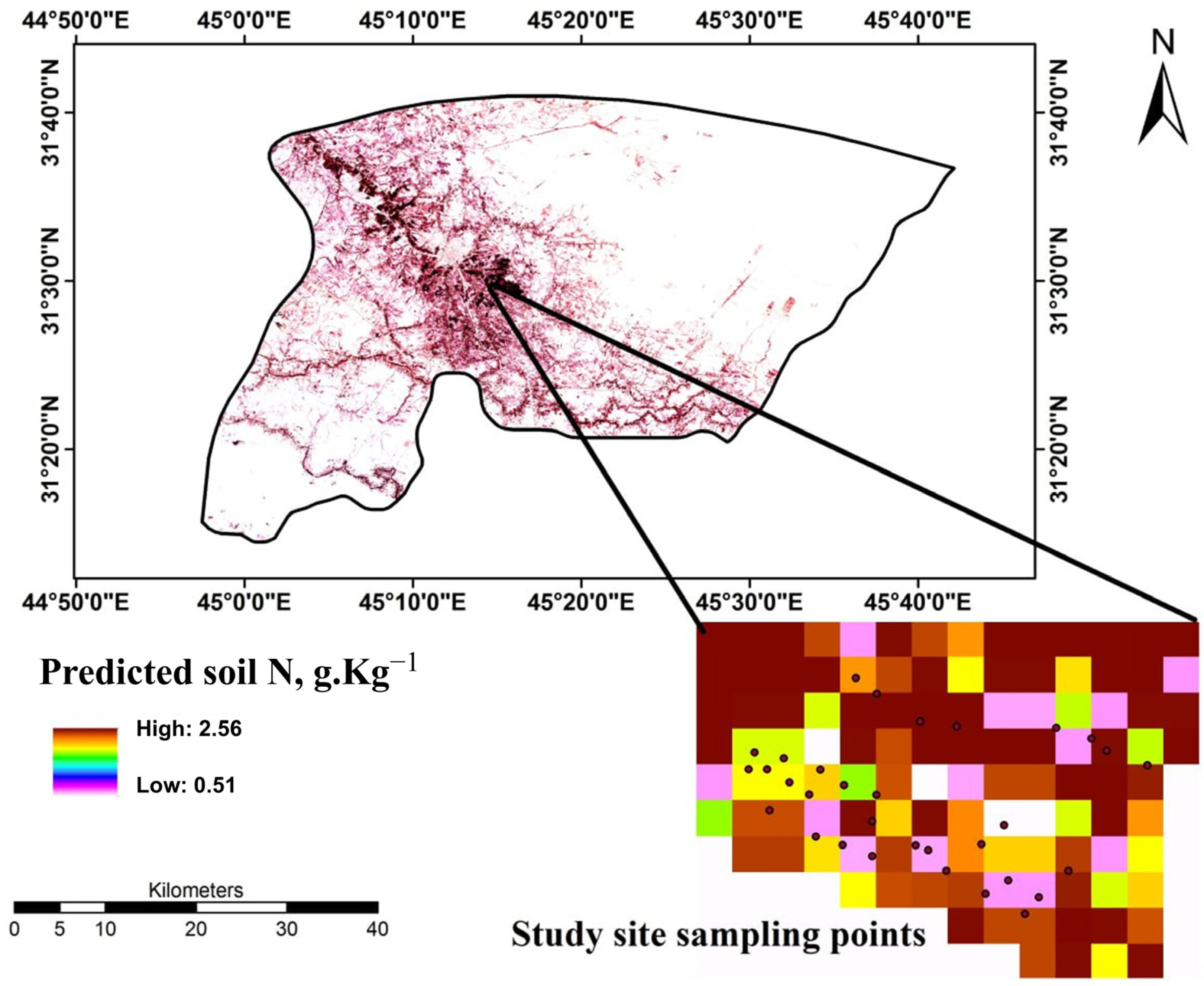
3.3. Spatial Characteristics of Soil N Prediction

The current study mapped the spatial distribution of total soil N content in a wheat field using the bootstrapped RF (log B5/B7) model (Figure 3). The graph indicated high predicted N content, with values reaching up to 2.564 g/kg, primarily located in areas of the wheat field characterized by fertile soils. In contrast, low predicted soil N values were observed, falling below 0.516 g/kg. The zoomed-in section of the graph illustrates the detailed variability of the predicted soil N values, while the points mark the locations of soil samples used for assessing model performance. The consistency between predicted and actual soil N values demonstrates the model’s predictive power; however, discrepancies may undermine confidence in the RF model. Overall, the model effectively illustrates the heterogeneity of soil N distribution within the studied area, showing a slight overestimate (bias of 0.0068) and a low deviation from actual soil N values (mean absolute error of 0.03).
Our results revealed a predominance of high soil N content at ground-truth points, likely attributable to existing agricultural practices, as the study site is a wheat field typically fertilized with N fertilizers (Figure 3). The potential of remote sensing to detect in-field soil N content was promising, although further research is needed across various environments. Several scientific studies have noted the effectiveness of remotely sensed mapping and the quantitative assessment of in-field soil property variations, achieving moderately accurate predictions [50,51].
The positive outcomes observed can be largely attributed to the low levels of organic matter and moisture content (Table 1), as these two soil properties are the most strongly correlated with soil reflectance. Research shows that both organic matter and moisture can significantly diminish the ability to accurately predict soil N levels. For example, a study by Cao et al. [52] emphasizes that organic matter affects the spectral response of soils, which in turn influences the retrieval of soil properties using reflectance techniques. Additionally, numerous studies, including those by [53], have established that high moisture content in soil can disrupt the spectral signature, resulting in reduced accuracy when predicting nutrient concentrations. Therefore, understanding the relationship between these properties and soil reflectance is essential for recognizing the limitations of predicting soil N content through remote sensing methods [54,55].
The ability to translate soil reflectance into management decisions remains a significant challenge for producers. Therefore, when predicting soil N spatially, it is essential to account for additional factors that influence spectral reflectance [56,57,58,59]. Harmonized remote sensing data, along with advanced statistical and machine learning algorithms, offer valuable insights and predictions regarding the spatial variability of soil N. The key advantages of this promising tool include detailed spatial information, rapid data collection, and the capability to cover extensive areas [60]. To enhance the accuracy of soil N estimation, future research could concentrate on refining the pre-treatment methods for spectral reflectance.
By utilizing advanced statistical techniques such as PCA, bootstrap resampling methods, and machine learning algorithms like RF, we enhanced the model’s predictive power for detecting soil N in diverse agricultural landscapes using multi-temporal spectral data from GEE. GEE’s capability to manage large datasets significantly aids in accounting for the complex interactions between vegetation, soil properties, and soil N spectral reflectance [61,62].

4. Conclusions

Our study highlighted the importance of bootstrapping in improving soil N prediction models for large-scale wheat fields. The results from the PCA identified bands 5 and 7 from Landsat 9 as significant, accounting for 91.3% of the variability in soil N across the selected wheat fields in the Al-Rumaitha district. Among the three RF models developed, the logarithmic band ratio demonstrated the best metrics for R2 and RMSE in both the bootstrapped and non-bootstrapped approaches. The utilization of several decision trees through the bootstrap aggregation method enhanced model performance, improving the R2 from 0.614 to 0.773, while slightly reducing RMSE values from 0.17 to 0.10. However, predicting low soil N levels remained challenging due to high variability. In summary, bootstrapping was effective in identifying outlier samples, reducing uncertainty in predictions.
We believe that the integration of advanced statistical and machine learning algorithms with satellite imagery on an open-access platform like GEE presents a valuable solution for soil fertility management by enhancing data quality and prediction accuracy. This approach offers a reliable solution for monitoring soil N levels in arid regions and can be scaled to incorporate diverse soil types and crops. Further research should investigate the specific site properties of these soil samples to assess their impact on prediction model accuracy, while future studies should broaden datasets to incorporate additional environmental factors and improve models for tracking soil N dynamics across diverse agricultural systems.

Author Contributions

Q.A.T.A.-S.: conceptualization, data curation, methodology, supervision, writing—original draft, and writing—review and editing. S.M.A.-H.: data curation, formal analysis, validation, writing—original draft, and writing—review and editing. M.A.N.: data curation, formal analysis, and writing—review and editing. S.M.S.: project administration and writing—review and editing. A.H.A.: methodology, resources, and writing—review and editing analysis. D.P.: validation, visualization, and writing—review and editing. All authors have read and agreed to the published version of the manuscript.

Funding

This research received no external funding.

Data Availability Statement

The data supporting the results of this study are available upon request to the corresponding author.

Acknowledgments

The authors sincerely gratitude to the College of Environmental Sciences at Al-Qasim Green University for supporting this research. We are also grateful to Google Earth Engine for granting its powerful cloud computing platform, which was essential in enabling data analysis and model development. Additionally, we extend our special thanks to the Al-Muthana state board of Agriculture Research, Ministry of Agriculture, Iraq for their assistance in localized data collection. Finally, we thank the anonymous reviewers and the academic editor for their valuable comments and suggestions, which helped improve this paper.

Conflicts of Interest

The authors declare no conflicts of interest.

References

  1. Mueller, N.D.; Gerber, J.S.; Johnston, M.; Ray, D.K.; Ramankutty, N.; Foley, J.A. Closing Yield Gaps through Nutrient and Water Management. Nature 2012, 490, 254–257. [Google Scholar] [PubMed]
  2. Zhang, X.; Wang, Y.; Schulte-Uebbing, L.; De Vries, W.; Zou, T.; Davidson, E.A. Sustainable Nitrogen Management Index: Definition, Global Assessment, and Potential Improvements. Front. Agric. Sci. Eng. 2022, 9, 507–521. [Google Scholar] [CrossRef]
  3. Gu, X.; Zhang, S.; Lam, S.K.; Yu, Y.; van Grinsven, H.J.M.; Zhang, S.; Wang, X.; Bodirsky, B.L.; Wang, S.; Duan, J.; et al. Cost-Effective Mitigation of Nitrogen Pollution from Global Croplands. Nature 2023, 613, 77–84. [Google Scholar] [CrossRef]
  4. Williams, D.R.; Clark, M.; Buchanan, G.M.; Ficetola, G.F.; Rondinini, C.; Tilman, D. Proactive Conservation to Prevent Habitat Losses to Agricultural Expansion. Nat. Sustain. 2021, 4, 314–322. [Google Scholar] [CrossRef]
  5. Naser, A.M.; Khosla, R.; Longchamps, L.; Dahal, S. Characterizing Variation in Nitrogen Use Efficiency in Wheat Genotypes Using Proximal Canopy Sensing for Sustainable Wheat Production. Agronomy 2020, 10, 773. [Google Scholar] [CrossRef]
  6. Zhang, X.; Davidson, E.A.; Mauzerall, D.L.; Searchinger, T.D.; Dumas, P.; Shen, Y. Managing Nitrogen for Sustainable Development. Nature 2015, 528, 51–59. [Google Scholar] [CrossRef]
  7. Wulder, M.A.; Masek, J.G.; Cohen, W.B.; Loveland, T.R.; Woodcock, C.E. Opening the Archive: How Free Data Has Enabled the Science and Monitoring Promise of Landsat. Remote Sens. Environ. 2012, 122, 2–10. [Google Scholar]
  8. Forkuor, G.; Hounkpatin, O.K.L.; Welp, G.; Thiel, M. High-Resolution Mapping of Soil Properties Using Remote Sensing Variables in Southwestern Burkina Faso: A Comparison of Machine Learning and Multiple Linear Regression Models. PLoS ONE 2017, 12, e0170478. [Google Scholar] [CrossRef]
  9. Naser, M.A.; Khosla, R.; Longchamps, L.; Dahal, S. Using NDVI to Differentiate Wheat Genotypes Productivity under Dryland and Irrigated Conditions. Remote Sens. 2020, 12, 824. [Google Scholar] [CrossRef]
  10. Yong, H.; Song, H.Y.; Garcia Pereira, A.; Hernandez Gomez, A. Measurement and analysis of soil nitrogen and organic matter content using near-infrared spectroscopy techniques. J. Zhejiang Univ. Sci. B 2005, 6, 1081–1086. [Google Scholar] [CrossRef]
  11. Ge, Y.; Morgan, C.L.S.; Grunwald, S.; Brown, D.J.; Sarkhot, D.V. Comparison of soil reflectance spectra and calibration models obtained using multiple spectrometers. Geoderma 2011, 161, 202–211. [Google Scholar] [CrossRef]
  12. An, X.; Li, M.; Zheng, L.; Liu, Y.; Sun, H. A portable soil nitrogen detector based on NIRS. Precis. Agric. 2014, 15, 3–16. [Google Scholar] [CrossRef]
  13. Al-Shujairy, Q.A.T.; Ali, N.S. Prediction of soil total nitrogen using spectroradiometer and GIS in southern Iraq. Int. J. Environ. Agric. Res. 2017, 3, 116–122. [Google Scholar]
  14. Dewitte, O.; Jones, A.; Elbelrhiti, H.; Horion, S.; Montanarella, L. Satellite Remote Sensing for Soil Mapping in Africa: An Overview. Prog. Phys. Geogr. 2012, 36, 514–538. [Google Scholar] [CrossRef]
  15. Xu, S.; Wang, M.; Shi, X.; Yu, Q.; Zhang, Z. Integrating Hyperspectral Imaging with Machine Learning Techniques for the High-Resolution Mapping of Soil Nitrogen Fractions in Soil Profiles. Sci. Total Environ. 2021, 754, 142135. [Google Scholar] [CrossRef] [PubMed]
  16. Liu, X.; Yang, J.; Yuan, L. Predicting the High Heating Value and Nitrogen Content of Torrefied Biomass Using a Support Vector Machine Optimized by a Sparrow Search Algorithm. RSC Adv. 2023, 13, 802–807. [Google Scholar] [CrossRef]
  17. Wang, S.; Jin, X.; Adhikari, K.; Li, W.; Yu, M.; Bian, Z.; Wang, Q. Mapping Total Soil Nitrogen from a Site in Northeastern China. Catena 2018, 166, 134–146. [Google Scholar] [CrossRef]
  18. Ye, Y.; Jiang, Y.; Kuang, L.; Han, Y.; Xu, Z.; Guo, X. Predicting Spatial Distribution of Soil Organic Carbon and Total Nitrogen in a Typical Human-Impacted Area. Geocarto Int. 2022, 37, 4465–4482. [Google Scholar] [CrossRef]
  19. Liu, J.; Yang, K.; Tariq, A.; Lu, L.; Soufan, W.; El Sabagh, A. Interaction of climate, topography and soil properties with cropland and cropping pattern using remote sensing data and machine learning methods. Egypt. J. Remote Sens. Space Sci. 2023, 26, 415–426. [Google Scholar] [CrossRef]
  20. Xu, Y.; Wang, L.; Ma, Z.; Li, B.; Bartels, R.; Liu, C.; Zhang, X.; Dong, J. Spatially Explicit Model for Statistical Downscaling of Satellite Passive Microwave Soil Moisture. IEEE Trans. Geosci. Remote Sens. 2020, 58, 1182–1191. [Google Scholar] [CrossRef]
  21. Dong, W.; Wu, T.; Luo, J.; Sun, Y.; Xia, L. Land Parcel-Based Digital Soil Mapping of Soil Nutrient Properties in an Alluvial-Diluvial Plain Agricultural Area in China. Geoderma 2019, 340, 234–248. [Google Scholar] [CrossRef]
  22. Kohavi, R. A Study of Cross-Validation and Bootstrap for Accuracy Estimation and Model Selection. In Proceedings of the 14th International Joint Conference on Artificial Intelligence (IJCAI), Montreal, QC, Canada, 20–25 August 1995; pp. 1137–1145. [Google Scholar]
  23. Zoubir, A.M.; Iskandler, D.R. Bootstrap Methods and Applications. IEEE Signal Process. Mag. 2007, 24, 10–19. [Google Scholar] [CrossRef]
  24. Hesterberg, T. Bootstrap. Wiley Interdiscip. Rev. Comput. Stat. 2011, 3, 497–526. [Google Scholar] [CrossRef]
  25. Efron, B.; Tibshirani, R.J. An Introduction to the Bootstrap; CRC Press: Boca Raton, FL, USA, 1994. [Google Scholar]
  26. Alesso, C.A.; Masola, M.J.; Carrizo, M.E.; Imhoff, S.D.C. Estimating sample size of soil cone index profiles by bootstrapping. Rev. Bras. Cienc. Solo 2017, 41, e0160464. [Google Scholar] [CrossRef]
  27. Harris, P.; Brunsdon, C.; Lu, B.; Nakaya, T.; Charlton, M. Introducing bootstrap methods to investigate coefficient nonstationarity in spatial regression models. Spat. Stat. 2017, 21, 241–261. [Google Scholar] [CrossRef]
  28. Dane, J.H.; Reed, R.B.; Hopmans, J.W. Estimating soil parameters and sample size by bootstrapping. Soil Sci. Soc. Am. J. 1986, 50, 283–287. [Google Scholar] [CrossRef]
  29. Li, D.-Q.; Tang, X.-S.; Phoon, K.-K. Bootstrap method for characterizing the effect of uncertainty in shear strength parameters on slope reliability. Reliab. Eng. Syst. Saf. 2015, 140, 99–106. [Google Scholar] [CrossRef]
  30. Hrba, M.; Maciak, M.; Peštová, B.; Pešta, M. Bootstrapping not independent and not identically distributed data. Mathematics 2022, 10, 4671. [Google Scholar] [CrossRef]
  31. Omondiagebe, O.P.; Roudier, P.; Liburne, L.; Ma, Y.; McNeill, S. Quantifying uncertainty in the prediction of soil properties using mid-infra spectra. Geoderma 2024, 448, 116954. [Google Scholar] [CrossRef]
  32. Cao, B.; Domke, G.M.; Russell, M.B.; Walters, B.F. Spatial modeling of litter and soil carbon stocks on forest land in the conterminous United States. Sci. Total Environ. 2019, 654, 94–106. [Google Scholar] [CrossRef]
  33. Maleki, S.; Karimi, A.; Mousavi, A.; Kerry, R.; Taghizadeh-Mehrjardi, R. Delineation of soil management zone maps at the regional scale using machine learning. Agronomy 2023, 13, 445. [Google Scholar] [CrossRef]
  34. Estefan, G.; Sommer, R.; Ryan, J. (Eds.) Methods of Soil, Plant, and Water Analysis: A Manual for the West Asia and North Africa Region, 3rd ed.; ICARDA: Beirut, Lebanon, 2013. [Google Scholar]
  35. Samarasinghe, S. Neural Networks for Applied Sciences and Engineering: From Fundamentals to Complex Pattern Recognition; Auerbach: Boca Raton, FL, USA, 2007. [Google Scholar]
  36. Efron, B. Better bootstrap confidence intervals. J. Am. Stat. Assoc. 1987, 82, 171–185. [Google Scholar] [CrossRef]
  37. Gasmi, A.; Gomez, C.; Chehbouni, A.; Dhiba, D.; Elfil, H. Satellite Multi-Sensor Data Fusion for Soil Clay Mapping Based on the Spectral Index and Spectral Bands Approaches. Remote Sens. 2022, 14, 1103. [Google Scholar] [CrossRef]
  38. Varshitha, D.N.; Choudhary, S. A Bootstrap Aggregation Approach for Adequate Crop Fertilizer and Nutrition Recommendation. Indones. J. Electr. Eng. Comput. Sci. 2022, 26, 1773–1780. [Google Scholar] [CrossRef]
  39. Bantigeza, M.K.; Tesfay, F.; Terefe, H.; Mezgebo, T. Land Use Land Cover Change and Habitat Vulnerability to Disturbance in Menz-Guassa Community Conservation Area, North Shewa, Ethiopia. Res. Sq. 2025. [Google Scholar] [CrossRef]
  40. Ali, M.; Ali, T.; Gawai, R.; Dronjak, L.; Elaksher, A. The Analysis of Land Use and Climate Change Impacts on Lake Victoria Basin Using Multi-Source Remote Sensing Data and Google Earth Engine (GEE). Remote Sens. 2024, 16, 4810. [Google Scholar] [CrossRef]
  41. Ablat, X.; Huang, C.; Tang, G.; Erkin, N.; Sawut, R. Modeling Soil CO2 Efflux in a Subtropical Forest by Combining Fused Remote Sensing Images with Linear Mixed Effect Models. Remote Sens. 2023, 15, 1415. [Google Scholar] [CrossRef]
  42. Li, H.; Li, D.; Xu, K.; Cao, W.; Jiang, X.; Ni, J. Monitoring of Nitrogen Indices in Wheat Leaves Based on the Integration of Spectral and Canopy Structure Information. Agronomy 2022, 12, 833. [Google Scholar] [CrossRef]
  43. Tan, K.; Wang, H.; Chen, L.; Du, Q.; Du, P.; Pan, C. Estimation of the Spatial Distribution of Heavy Metals in Agricultural Soils Using Airborne Hyperspectral Imaging and Random Forest. J. Hazard. Mater. 2020, 382, 120987. [Google Scholar] [CrossRef]
  44. Belgiu, M.; Drăguţ, L. Random forest in remote sensing: A review of applications and future directions. ISPRS J. Photogramm. Remote Sens. 2016, 114, 24–31. [Google Scholar] [CrossRef]
  45. Sheikholeslami, R.; Hall, J.W. A Global Assessment of Nitrogen Concentrations Using Spatiotemporal Random Forests. Hydrol. Earth Syst. Sci. Discuss. 2022, 2022, 1–22. [Google Scholar] [CrossRef]
  46. Dhaliwal, J.K.; Panday, D.; Robertson, G.P.; Saha, D. Machine learning reveals dynamic controls of soil nitrous oxide emissions from diverse long-term cropping systems. J. Environ. Qual. 2024, 54, 132–146. [Google Scholar] [CrossRef]
  47. Francis, H.R.; Ma, T.F.; Ruark, M.D. Toward a standardized statistical methodology comparing optimum nitrogen rates among management practices: A bootstrapping approach. Agric. Environ. Lett. 2021, 6, e20045. [Google Scholar] [CrossRef]
  48. Cui, H.; Xu, Z.; Wang, Y. Data preprocessing and machine learning algorithms for soil nitrogen prediction: A comparative study. Ecol. Inform. 2020, 57, 101066. [Google Scholar]
  49. Zhang, L.; Wu, Z.; Sun, X.; Yan, J.; Sun, Y.; Liu, P.; Chen, J. Mapping topsoil total nitrogen using random forest and modified regression kriging in agricultural areas of central China. Plants 2023, 12, 1464. [Google Scholar] [CrossRef]
  50. Peng, Y.; Xiong, X.; Adhikari, K.; Knadel, M.; Grunwald, S.; Greve, M.H. Modeling Soil Organic Carbon at Regional Scale by Combining Multi-Spectral Images with Laboratory Spectra. PLoS ONE 2015, 10, e0142295. [Google Scholar] [CrossRef] [PubMed]
  51. Yang, Y.; Shang, K.; Xiao, C.; Wang, C.; Tang, H. Spectral Index for Mapping Topsoil Organic Matter Content Based on ZY1-02D Satellite Hyperspectral Data in Jiangsu Province, China. ISPRS Int. J. Geo-Inf. 2022, 11, 111. [Google Scholar] [CrossRef]
  52. Cao, S.J.; Zhu, X.C.; Li, C.; Wei, Y.; Guo, X.Y.; Yu, X.Y. Estimating Total Nitrogen Content in Brown Soil of Orchard Based on Hyperspectrum. Open J. Soil Sci. 2017, 7, 203–215. [Google Scholar] [CrossRef]
  53. Lesaignoux, A.; Fabre, S.; Briottet, X. Influence of soil moisture content on spectral reflectance of bare soils in the 0.4–14 µm domain. Int. J. Remote Sens. 2013, 34, 2268–2285. [Google Scholar] [CrossRef]
  54. Datta, D.; Paul, M.; Murshed, M.; Teng, S.W.; Schmidtke, L. Soil moisture, organic carbon, and nitrogen content prediction with hyperspectral data using regression models. Sensors 2022, 22, 7998. [Google Scholar] [CrossRef]
  55. Li, T.; Mu, T.; Liu, G.; Yang, X.; Zhu, G.; Shang, C. A method of soil moisture content estimation at various soil organic matter conditions based on soil reflectance. Remote Sens. 2022, 14, 2411. [Google Scholar] [CrossRef]
  56. Peri, P.L.; Rosas, Y.M.; Ladd, B.; Toledo, S.; Lasagno, R.G.; Pastur, G.M. Modeling Soil Nitrogen Content in South Patagonia Across a Climate Gradient, Vegetation Type, and Grazing. Sustainability 2019, 11, 2707. [Google Scholar] [CrossRef]
  57. Zhang, Y.; Sui, B.; Shen, H.; Ouyang, L. Mapping Stocks of Soil Total Nitrogen Using Remote Sensing Data: A Comparison of Random Forest Models with Different Predictors. Comput. Electron. Agric. 2019, 160, 23–30. [Google Scholar] [CrossRef]
  58. Alemu, L.; Mesfin, B. Performance of Mid-Infrared Spectroscopy to Predict Nutrients for Agricultural Soils in Selected Areas of Ethiopia. Heliyon 2022, 8, e09050. [Google Scholar] [CrossRef]
  59. Dai, L.; Ge, J.; Wang, L.; Zhang, Q.; Liang, T.; Bolan, N.; Lischeid, G.; Rinklebe, J. Influence of Soil Properties, Topography, and Land Cover on Soil Organic Carbon and Total Nitrogen Concentration: A Case Study in Qinghai-Tibet Plateau Based on Random Forest Regression and Structural Equation Modeling. Sci. Total Environ. 2022, 821, 153440. [Google Scholar] [CrossRef] [PubMed]
  60. Xu, J.; Liu, Y.; Yan, C.; Yuan, J. Estimation of Soil Organic Matter Based on Spectral Indices Combined with Water Removal Algorithm. Remote Sens. 2024, 16, 2065. [Google Scholar] [CrossRef]
  61. Auzzas, A.; Capra, G.F.; Jani, A.D.; Ganga, A. An Improved Digital Soil Mapping to Predict Nitrogen by Combining Machine Learning Algorithms and Open Environmental Data. Model. Earth Syst. Environ. 2024, 10, 6519–6538. [Google Scholar] [CrossRef]
  62. Stefano, C.D.; Ferro, V.; Porto, P. Applying the Bootstrap Technique for Studying Soil Redistribution by Caesium-137 Measurements at Basin Scale. Hydrol. Sci. J. 2000, 45, 171–183. [Google Scholar] [CrossRef]
Figure 1. Framework for the total soil N variability prediction.
Nitrogen 06 00023 g001
Figure 2. Bootstrap (ac) and non-bootstrap (df) based (RF) models constructed with the ratio (B5/B7) for model 1, log (B5/B7) for model 2, and 1/log (B5/B7) for model 3.
Nitrogen 06 00023 g002
Figure 3. The distribution of total soil N contents based on the bootstrapped RF log (B5/B7) model in the Al-Rumaitha district and zoomed-in section of the study site.
Nitrogen 06 00023 g003
Table 1. A summary of measured soil properties from the study area.
Soil PropertyValueUnit
Electrical conductivity (ECe)8.7dS.m−1
pH7.5
Soil organic matter (OM)8g.Kg−1
Soil textureSandy clay loam
Soil moisture10%
Table 2. Eigenvectors of the covariance matrix of the principal component transformation.
Principal ComponentBand 2Band 3Band 4Band 5Band 6Band 7EigenvalueVariance
Explained%
PC10.380.09−0.57−0.580.460.421.2025.12
PC20.40−0.05−0.390.060.08−0.820.9920.84
PC30.44−0.3−0.210.72−0.220.381.0421.71
PC50.520.150.390.090.070.030.469.59
PC60.48−0.580.56−0.35−0.29−0.031.0922.74
Table 3. Accuracy evaluation metrics of bootstrapping- and non-bootstrapping-based random forest models.
BootstrappingMeanR2RMSEConfidence Intervals *
B5/B70.860.4890.350.074–0.2157
Log (B5/B7)0.890.7730.100.723–1.0263
1/(Log B5/B7)−0.150.1911.07−0.6954–0.6225
Non-BootstrappingMeanR2RMSE
B5/B70.870.4010.69
Log (B5/B7)0.870.6140.17
1/(Log B5/B7)−0.140.1131.42
* The confidence intervals (95%) are computed only for the mean under bootstrap-based models.
Disclaimer/Publisher’s Note: The statements, opinions and data contained in all publications are solely those of the individual author(s) and contributor(s) and not of MDPI and/or the editor(s). MDPI and/or the editor(s) disclaim responsibility for any injury to people or property resulting from any ideas, methods, instructions or products referred to in the content.

