Abstract
Chronic elevated nitrogen (N) deposition can have adverse effects on terrestrial ecosystems. For large areas of northern Canada distant from emissions sources, long-range atmospheric transport of N may impact plant species diversity, even at low deposition levels. The objective of this study was to establish plant species community thresholds for N deposition under multiple environmental gradients using gradient forest analysis. Plant species abundance data for 297 Jack pine (Pinus banksiana Lamb.)-dominant forest plots across Alberta and Saskatchewan, Canada, were evaluated against 43 bioclimatic and deposition variables. Bioclimatic variables were overwhelmingly the most important drivers of community thresholds. Nonetheless, dry N oxide (DNO) and dry N dioxide deposition inferred a total deposited N (TDN) community threshold of 1.4–2.1 kg N ha−1 yr−1. This range was predominantly associated with changes in several lichen species, including Cladina mitis, Vulpicida pinastri, Evernia mesomorpha and Lecanora circumborealis, some of which are known bioindicators of N deposition. A secondary DNO threshold appeared to be driving changes in several vascular species and was equivalent to 2.45–3.15 kg N ha−1 yr−1 on the TDN gradient. These results suggest that in low deposition ‘background’ regions a biodiversity-based empirical critical load of 1.4–3.15 kg N ha−1 yr−1 will protect lichen communities and other N-sensitive species in Jack pine forests across Northwestern Canada. Nitrogen deposition above the critical load may lead to adverse effects on plant species biodiversity within these forests.
1. Introduction
The intensification of anthropogenic activity during the last century has led to a rise in atmospheric emissions and the deposition of many pollutants including nitrogen (N), the effects of which have been studied across local, regional, and global scales [1,2,3]. In Canada, agriculture, transportation, and industry, including oil and gas and other utilities, are the dominant sources of N emissions, with transportation (via road, rail, air, and marine) and the oil and gas industry accounting for almost 70% of all emissions [4]. In eastern Canada, nitrogen oxide (NO×) emissions were reduced by 26% from 1990 to 2017 due to international agreements and national efforts [4,5]; however, emissions in the west have remained high, with Alberta alone accounting for 27% of all national ammonia (NH3) emissions and 36% of all NO× emissions in 2017 [4].
Increases in N emissions (both reduced and oxidized N) can affect terrestrial ecosystems and has been widely recognized as a key driver of changing plant species diversity [6,7,8]. Even at low levels, chronic N deposition can have adverse effects through direct foliar changes and increased susceptibility to secondary stressors. It can also lead to soil acidification, eutrophication, and shift entire ecosystems to a point of N saturation, favouring more N-tolerant species, and ultimately reducing biodiversity [1,3,9,10,11,12]. Jack pine (Pinus banksiana Lamb.) coniferous forests are a predominant stand across almost 80% of boreal forests in Canada (preceded only by spruce and poplar stands, [13]). Moreover, Jack pine stands tend to have nutrient-poor, well-drained soils that range from coarse to fine sands or gravel [14] and are generally accompanied by an N-sensitive understory composed of a variety of lichen, bryophytes, and dwarf shrubs [8,15].
Assessing the effects of N deposition on sensitive terrestrial environments is widely carried out using critical loads [16,17,18,19], which have been used to underpin emissions reductions policies. Critical loads can be established through a variety of methods: empirically using observational data; a steady-state mass balance approach that estimates the loss or accumulation of N inputs and outputs over the long term; or dynamic modelling that includes time-dependent processes [20,21]. Empirical critical loads of nutrient N (CLempN) are based on environmental responses to N and infer a level below which no adverse effects occur [22,23,24].
In Europe, CLempN have been published according to the European Nature Information System (EUNIS), which defines different ecosystems based on dominant tree species, soil hydrology, and management practices [23,24]. In a review of gradient and experimental N-addition studies, coniferous woodland forests (EUNIS, class T3) had a recommended range of 3–15 kg N ha−1 yr−1, with exceedance defined by changes in soil processes, nutrient imbalances, altered composition mycorrhiza, and ground vegetation [24]. In many studies, CLempN from the 2010 UNECE workshop [23] are extrapolated to similar ecosystems [20]; however, some European forests have been known to experience as much as 100 kg N ha−1 yr−1, levels much greater than have historically been seen across large regions of Alberta and Saskatchewan [15]. A similar review in northern United States [20] recommended a range of 3–8 kg N ha−1 yr−1 for nutrient N deposition in hardwood and coniferous northern forests [20]. In Canada, recommended critical loads for coniferous forests have been set between 5–10 kg N ha−1 yr−1, with exceedance marked by changes in ground cover and increases in foliar and soil N concentration [15]. Despite differences in published CLempN for coniferous and mixedwood forests, changing ground species biodiversity has remained a constant indication of exceedance.
Thresholds for N deposition can be identified using several methods based on the data availability [22,23,24]. Long-term field additions and targeted N experiments have been used to inform CLempN [25,26,27] but gradient studies have also been effective in quantifying CLempN [24]. Studies have assessed CLempN using survey data and applied general additive models (GAMs) to identify important community thresholds across a given habitat [28,29], while others have relied on regressions to establish terrestrial N deposition thresholds [30]. Regressions techniques have also been used to derive critical loads on a European scale through a vegetation-based model called Probability of Plant Species (PROPS), where plant species observational data were evaluated as a function of multiple abiotic environmental variables [31]. Gradient studies using Threshold Indicator Taxon Analysis (TITAN) have been used to evaluate changes in individual plant species abundance in European grasslands along an N gradient [32], and habitats in Ireland classified as high conservation importance (Annex I under the Habitats Directive), with changepoints inferring CLempN but only when they included positive indicator species previously identified by the National Parks and Wildlife Service [33]. Similar ecological thresholds have been determined for vegetation communities (i.e., alliances) across the United States [19].
In 2010, a novel approach was developed to examine community thresholds that sought to address several deficiencies in existing methods. Gradient forest analysis [34], is an extension of random forest analysis [35], a method that fits multiple regression tree models between individual species abundances and environmental variables [36]. However, gradient forest analysis was developed to be a more flexible, non-linear, multivariate approach, addressing multi-species threshold responses and establishing where in the gradient range compositional changes occur [36,37,38]. In this respect, gradient forest analysis is like TITAN, but it also accommodates multiple environmental variables and identifies their importance with respect to changes in plant species composition [34,36,38].
The objective of this study was to evaluate whether N deposition is a significant driver of changing plant species composition across Jack pine-dominant forests in northwestern Canada. Plant species abundance data for 297 plots across Alberta and Saskatchewan were evaluated against 43 environmental variables using gradient forest analysis to determine the importance of N as a driver of community level changes. Furthermore, gradient forest analysis was used to identify where community thresholds occurred across the gradient of environmental variables and the species that were particularly vulnerable. These results were used to infer an CLempN for Jack pine dominant forests.
2. Materials and Methods
2.1. Study Area
Study sites were selected across the province of Alberta and Saskatchewan, covering an area of approximately 270,000 km2. Study sites were predominantly located across the Boreal Plains and Boreal Shields ecozones, with additional sites located across the Taiga Shield ecozone. The Boreal Shield ecozone, stretching from Newfoundland to Alberta and covering roughly 1.8 million km2 and 2/3 of the province of Alberta, is defined by long cold winters and short warm summers [39,40]. The Boreal Plains ecozone covers 650,000 km2, is representative of a moist climate, and is defined by cold winters and moderately warm summers [39,40]. The Taiga shield is characterized by short, cool summers and long cold winters, and covers approximately 1.3 million km2 across Canada with some sections of northern Alberta and northern Saskatchewan falling into this ecozone [39,40]. Across both the Boreal Plains and the Boreal Shield, yearly precipitation averages around 400 mm, while the Taiga Shield, which has characteristically low yearly precipitation, ranges between 175 to 200 mm [39,40]. Jack pine is identified as a main conifer species across all three ecozones; however, stands are known to be stunted across the Taiga shield.
2.2. Data Sources
Plant species, including vascular, bryophyte, and lichen abundance data (recorded as percent cover) were obtained from three separate surveys with established semi-permanent and permanent monitoring plots across Alberta and Saskatchewan. Data from Alberta were obtained primarily from the Wood Buffalo Environmental Association (WBEA, [41]) while the Forest Ecosystem Classification Guide (SK-FEC, [42]) was used for most of the Saskatchewan data. In addition, the National Forest Inventory (NFI, [43]) provided data for 10 sites across Alberta and Saskatchewan. Initial WBEA data collection began in 1998 but over time, both sampling plots and methods were updated to accommodate both natural and anthropogenic changes to the landscape, including fires and construction [41]. The WBEA survey consisted of 25 Jack pine dominant, enhanced forest health network plots measuring 10 m by 40 m. Plant species and soil data were collected within small, medium, and large subplots across each site [41]. Across Saskatchewan, SK-FEC data were collected from 1700 semi-permanent, 10 m by 10 m plots and included species cover-abundance data as well as soil and site characteristics [42]. Survey data collection for the NFI began in 2001 with subsequent re-sampling efforts to occur over 10-year periods. The NFI has 1115 permanent plots set in a grid system across the country, each measuring 20 km × 20 km and within each permanent plot, a ground plot measuring 10 m by 10 m was established to identify ground vegetation and estimate percent cover [44]. For additional plot information, see the Supplementary Materials SI.
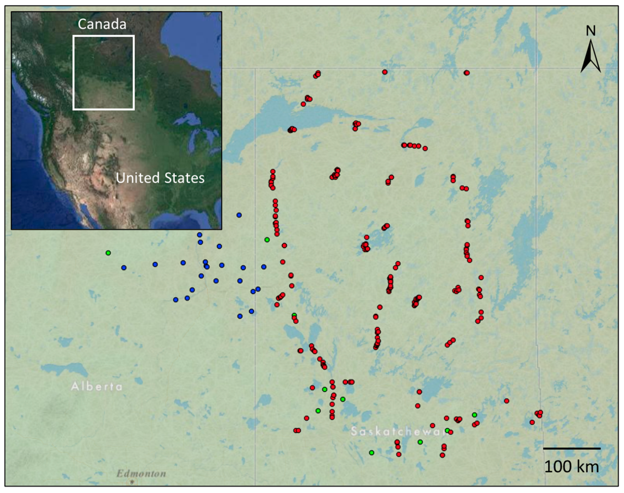
Across all three surveys, sites were only selected for analysis if the canopy coverage was classified as Jack pine-dominant, which was determined by evaluating the percentage of Jack pine coverage against total canopy coverage within a site. A site was only considered for the study if total canopy coverage was 10% or more of the site and of that, Jack pine comprised 50% or more of the stand. In total, 297 sites were selected across Alberta and Saskatchewan (Figure 1). Although disturbance data were not consistent across surveys, sampling criteria ensured that the selected sites were not recently subjected to forest fire disturbance, with SK-FEC ensuring sites were at least 40 years post-fire, WBEA ensured approximately 60 years post-fire disturbance in their sampling criteria, and the NFI reporting a minimum of 30 years post-fire disturbance.
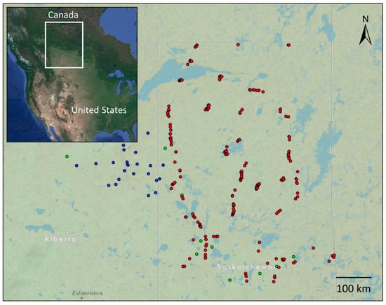
Figure 1.
Location of study sites across Alberta and Saskatchewan (n = 297) used in gradient forest analysis. Study sites are coloured based on their survey of origin, with blue indicating WBEA survey sites (n = 25), sampled between 2011 and 2012, green indicating NFI survey sites (n = 10), sampled between 2002 and 2006, and red indicating SK-FEC survey sites (n = 262), sampled between 2000 and 2010. The inset depicts the location of the study area in north America.
2.3. Environmental Data
Modelled estimates of N and sulphur (S) deposition data (in eq ha−1 yr−1) were obtained from GEM-MACH (Global Environmental Multi-Scale Modelling Air Quality and Chemistry); data were obtained at a resolution of 2.5 km × 2.5 km and based on emissions inventories from 2013 and 2014 [45]. Nitrogen deposition data, which included total deposited nitrogen (TDN), accounted for 12 different forms of N (Table 1) while S deposition accounted for four different S species (Table 1) and included total deposited sulphur (TDS). In addition, 23 bioclimatic variables (predictors) based on long-term climate normals were included in the analysis, as was elevation, longitude, and latitude (Table 2, [46]). In total, 43 different environmental variables were analyzed using gradient forests.

Table 1.
List of nitrogen and sulphur species (n = 17) and their associated summary statistics across all 297 study sites (see Figure 1). Data source: GEM-MACH [45].

Table 2.
List of location and bioclimatic variables (n = 26) and their associated summary statistics. Note that codes beginning in ‘bio’ are from Bioclim data and codes beginning in ‘sg’ are from Seedgrow data [46].
2.4. Statistical Analysis
Gradient forest analysis was performed in R studio using two packages: extendedForest and gradientForest. In the extendedForest package, a forest of regression trees (or classification trees if the data is binary) is constructed. During construction, a random sample of observations (termed in-bag observations) is fitted for each tree and response data is split into two groups along a gradient, with each split forming two branches and eventually a full tree [36,38]. A forest is created by repeating the construction of a single tree many times over and is done to reduce the instability of a single tree [36]. The number of trees in a forest is a call that can be set in the gradientForest package.
A branch in a tree is created by partitioning data according to a certain split value (s) for a given predictor (p), where sites to the left of the split value s have a predictor value p, below or equal to s, while those to the right have a predictor value above the split value [34,36,38]. Partitions in the data are done to maximize homogeneity in groupings, with respect to the response variable (e.g., one species’ abundance) and are repeated until only a minimum number of sites in the partition is reached, eventually forming a terminal node, where the predicted value is equivalent to the mean response of the node [34]. The split value s is selected so as to minimize the sum-of-squares deviation of the species abundance data (impurity) and in-turn maximizing the fit improvement (also known as reducing impurity). The fit improvement is a measure of how much the overall model variance has been explained by that partition and determines the importance of a split [34,36,47]. Each split can be interpreted as a response data threshold or changepoint, where a particular species (response data) may be present above this threshold but not below and vice versa for other species [34]. This process results in raw importance values that are then given to each predictor at a split value s in a particular tree for species f [36,38].
Observations not used in the construction of a tree are termed out-of-bag observations (OOB) and provide an estimate of the generalization error, the expected variance of the residuals for the new observation [34]. For each observation, the OOB prediction is the average of all predictions on all trees where the observation was OOB [34]. OOB predictions are used to cross validate the performance of a single tree, while the mean cross validated performance of all trees results in the goodness-of-fit measure [34,38]. The goodness-of-fit measure (also known as the predictive performance R2S values) produced in extendedForest represent, for each indicator (species), the proportion of variance explained by the random forest model [34,48]. Predictive performance values are calculated by comparing the generalization error in the model with the variance of observations (in other words, comparing a model without a given predictor to the full model). While it is possible for this value to be 0 (where generalization error exceeds the observed variance), the end result is the associated variable is determined to have no predictive power [34,36,48].
Accuracy importance values are also defined in extendedForest and are a measure of prediction accuracy in the model. Accuracy importance values are produced by assessing the importance values of each variable and their respective contribution to the overall model’s goodness-of-fit and are analogous to an increase in mean square error of OOB observations [48]. Accuracy importance informs on whether a variable has true predictive power or not and is measured by how much removing a variable will decrease (or increase) model accuracy. Relatively large accuracy importance values represent true predictive power for a variable, while small or negative values indicate that the environmental variable explain very little or nothing [34,48].
The ‘extendedForest’ package adopts similar functions from Breiman’s random forest models [35] and while random forest is known to perform well with high-dimensional data [49], additional measures such as the use of conditional permutations further increase model effectiveness when processing a large quantity of predictors by attempting to reduce collinearity between them. Conditional permutations allow for the assessment of the effects on the model when a given predictor is not considered, and as such the comparison of the prediction accuracy before and after the permutation of a conditional variable can be used as an importance measure [36,49]. Unlike marginal permutations, conditional permutations are permuted within bins of data defined by tree splits for predictors that are correlated above a specific threshold value that can be set in the gradientForest call [36,38,47].
GradientForest will then combine data from extendedForest, produce additional measures, and provide graphical outputs for specific measures to help evaluate community thresholds. Overall R2-weighted importance values are one such measure provided by gradientForest. R2-weighted importance is a measure of conditional importance and classifies the importance of each environmental variable with respect to community composition [38]. This is produced when gradientForest partitions the predictive performance R2S values (from extendedForest) into contributions (R2SP) from each predictor in proportion to the predictor importance. These contributions (R2SP) are then averaged across all species to provide the R2-weighted importance values for each predictor [48]. The mean R2-weighted importance value is the average of all R2-weighted importance values and is a measure of how much species variation in the entire model was explained by all predictors [38]. Compositional turnover functions for each predictor are then produced when gradientForest distributes the predictive performance values (R2S, calculated in extendedForest) for all species attributed to a given predictor gradient (environmental variables, [34,48]).
2.5. GradientForest Output
The output from gradient forest analysis includes several important statistical values and plots that can be used to identify the response for both individual plant species and the community across environmental gradients. To evaluate individual species variance, gradientForest produces R2 performance values for each environmental variable specific to each species (R2S). The sum of all specific R2S importance values within each species provides the R2 overall importance values, which is an indication of how well overall variance within each individual species was predicted by all environmental variables. Although values that are negative or zero are numerically possible for R2 overall performance, they are not included for further threshold analysis [50].
In addition to information at the individual species level, gradientForest produces several graphical outputs that provide information relating to the overall community composition. A plot depicting accuracy importance and R2-weighted importance visually classifies the importance of all environmental variables in relation to overall changing community composition as well as the model predictive power for each predictor (accuracy importance). Additional plots, including the densities plot and cumulative importance plots, serve to identify potential community-level thresholds across predictor gradients, and which species were particularly responsive within a given range [34,36,38]. Results for both the densities plot and the cumulative community plot are then plotted as non-linear, smoothed curves as gradientForest re-expresses split improvements from the random forest and extendedForest components with respect to both their contribution to total variance explained by the predictors and the contribution of each species in quantifying compositional change proportional to the variance explained by the predictors [36].
A densities plot identifies regions across an environmental gradient of higher importance for plant species compositional change and is estimated as the ratio of density of split importance to the density of observed predictor values along the given predictor gradient [48]. The black curve represents the density of splits, the red curve represents the density of data, while the blue curve represents the ratio of split-over data densities and grey histogram bars (binned split importance values) represent both split locations and relative importance on the gradient [36,38]. Peaks in the ratio of densities curve (where the blue line is greater than 1) indicate threshold values for that environmental variable [36] where relatively large changes in community composition occur. The distribution shown in each densities plot integrates to variable importance [38]. In cumulative importance plots, the cumulative compositional change along each gradient (in R2 units) is calculated by aggregating the normalized splits as cumulative distributions and are scaled by R2-weighted importance, standardized by the density of observations, and averaged across all species [36,48]. These plots display the same community thresholds seen in the densities plot but will display them in relation to all species data, identifying species that might be associated to large community shifts across the gradient [34,36,38].
Plant species abundance data for Jack pine dominant sites was evaluated against 43 environmental variables (Table 1 and Table 2). Initially, abundance data for 357 sites across all three surveys was used in gradientForest, however results revealed that longitude and latitude were the top environmental predictors and predictor importance for all other variables was considerably lower. In this initial analysis, several important thresholds were identified, representing a possible geographic bias in the data, with 2 thresholds for latitude at 60° and 54° and a single threshold for longitude at −115°. To increase uniformity, following previous studies [38,50] data were truncated to exclude any sites north of 60°, west of −115° and south of 54°, and a second analysis was performed, leaving 297 sites (nSK = 271 and nAB = 26, Figure 1) across Alberta and Saskatchewan. Species data for those sites included percent cover abundance, and species occurring at fewer than 3 sites were considered rare and removed from analysis. Overall, plant species abundance data for 218 species (nlichen = 96, nbryophyte = 41, nvascular = 79 and nfungi = 2) was included in the gradient forest analysis. Given the inherent importance some geographic and bioclimatic variables play in species composition [38,51,52], the focus of gradient forest analysis was placed on variables that were both classified as having high importance with respect to changing plant species composition and that are influenced by human activity. For additional information, see Supplementary Materials SII and SIII.
3. Results
Modelled estimates of TDN ranged from 31.2–597.0 eq ha−1 yr−1, while TDS ranged from 23.8–1182.2 eq ha−1 yr−1 (Table 1). Mean TDN was 105.9 eq ha−1 yr−1 (Table 1) and of the 297 sites, 108 sites received greater deposition than the mean. Annual precipitation (bio_12) ranged from 349–561 mm, with an average of 458 mm (Table 2). Annual mean temperature (sg_12) across the study area ranged from –5.46–1.64 °C (mean = −1.09 °C, sd = 1.46 °C, Table 2), while elevation ranged from 210.0–733.6 m (mean = 439.5 m, sd = 92.1 m, Table 2).
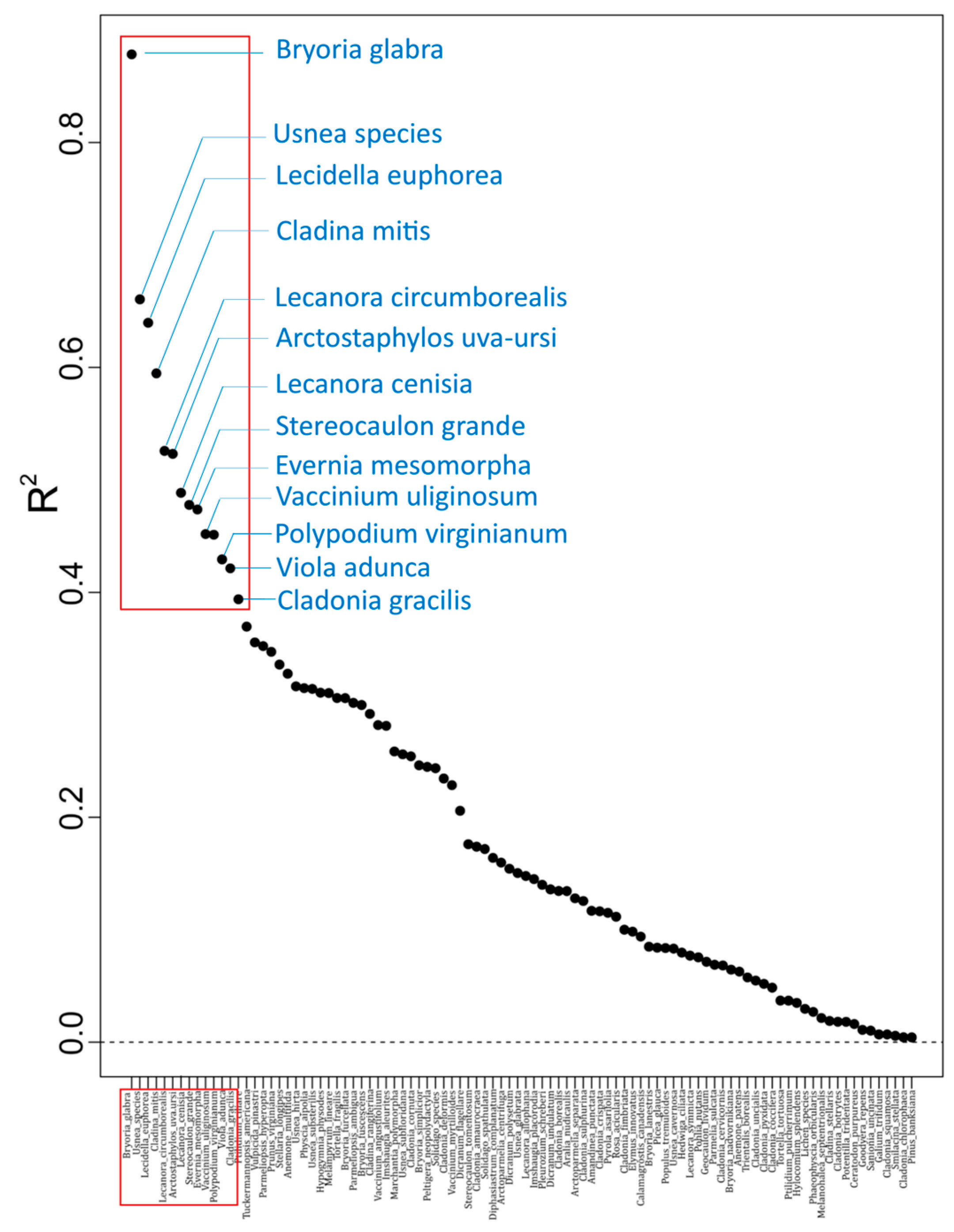
Of the 218 species evaluated in gradient forest analysis, 96 species had a positive R2 overall importance value, and of these, 13 species had a greater R2 measure of fit of their associated random forest model (R2 overall importance > 0.4, Figure 2, Table 3), meaning these species were particularly well predicted by the 43 environmental variables. Amongst the top-predicted species (R2 > 0.4), recurring environmental variables with highest R2S performance values (Table 3) were: longitude, total precipitation for period 1 (sg_04), total precipitation for period 3 (sg_06), wet hydrogen sulfite (HSO3), dry nitrogen oxide (DNO), TDS, and total precipitation for period 4 (sg_07).
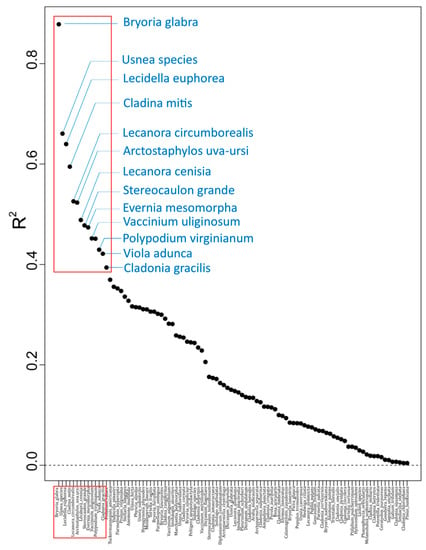
Figure 2.
Species R2 overall performance, a measure of the fit of random forest model for each species, with all 96 species with positive R2 values labelled on the X axis. The red outline identifies 13 species that were particularly well predicted by the environmental variables (R2 > 0.4). Species with zero or negative R2 overall performance values are not included.

Table 3.
R2 overall importance, the sum of R2S performance values for all environmental variables across a given species, for top 13 species (R2 > 0.4). Specific R2 performance values (R2S) for the top five environmental variables associated to each species.
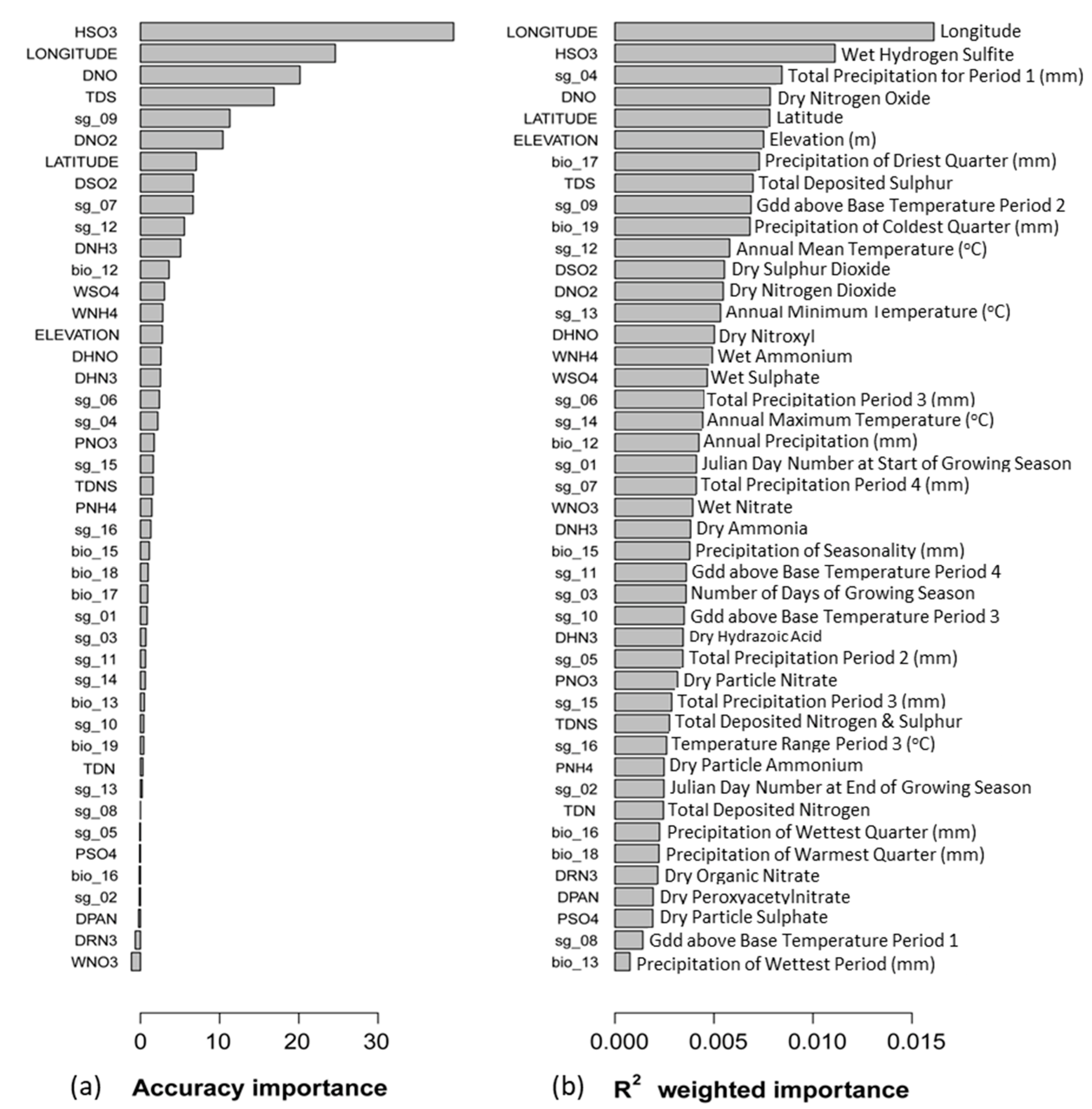
Mean accuracy importance was greatest for wet hydrogen sulfite (HSO3: 39.53, Figure 3) but rapidly reduced for all variables after dry nitrogen dioxide (DNO2 at 10.417, Figure 3). This suggests that variables with accuracy importance below DNO2 have very little predictive power, indicating that model accuracy would be altered very little or not at all if any of these variables were removed. Individual R2-weighted importance and mean R2-weighted importance (R2 = 0.00467, Table 4) were relatively low, indicating that the environmental variables explained a relatively small portion of the out-of-bag variation in the abundance data [48,53].

Figure 3.
(a) Mean accuracy importance. A higher mean accuracy importance value indicates greater predictive power for the environmental variable, while lower values indicate the predictor explains very little. Accuracy importance values are normalized to sum to the specific R2. (b) R2-weighted importance, shows the overall conditional importance of environmental variables for changing community composition. R2-weighted importance is calculated by weighting the species-level predictor importance by the species R2. Codes refer to environmental variables in Table 1 and Table 2.

Table 4.
R2-weighted importance values for top 15 environmental variables in decreasing order (left and right column) with mean R2-weighted importance of all environmental variables. R2-weighted importance values are the average of all R2S performance values for all species for each given predictor.
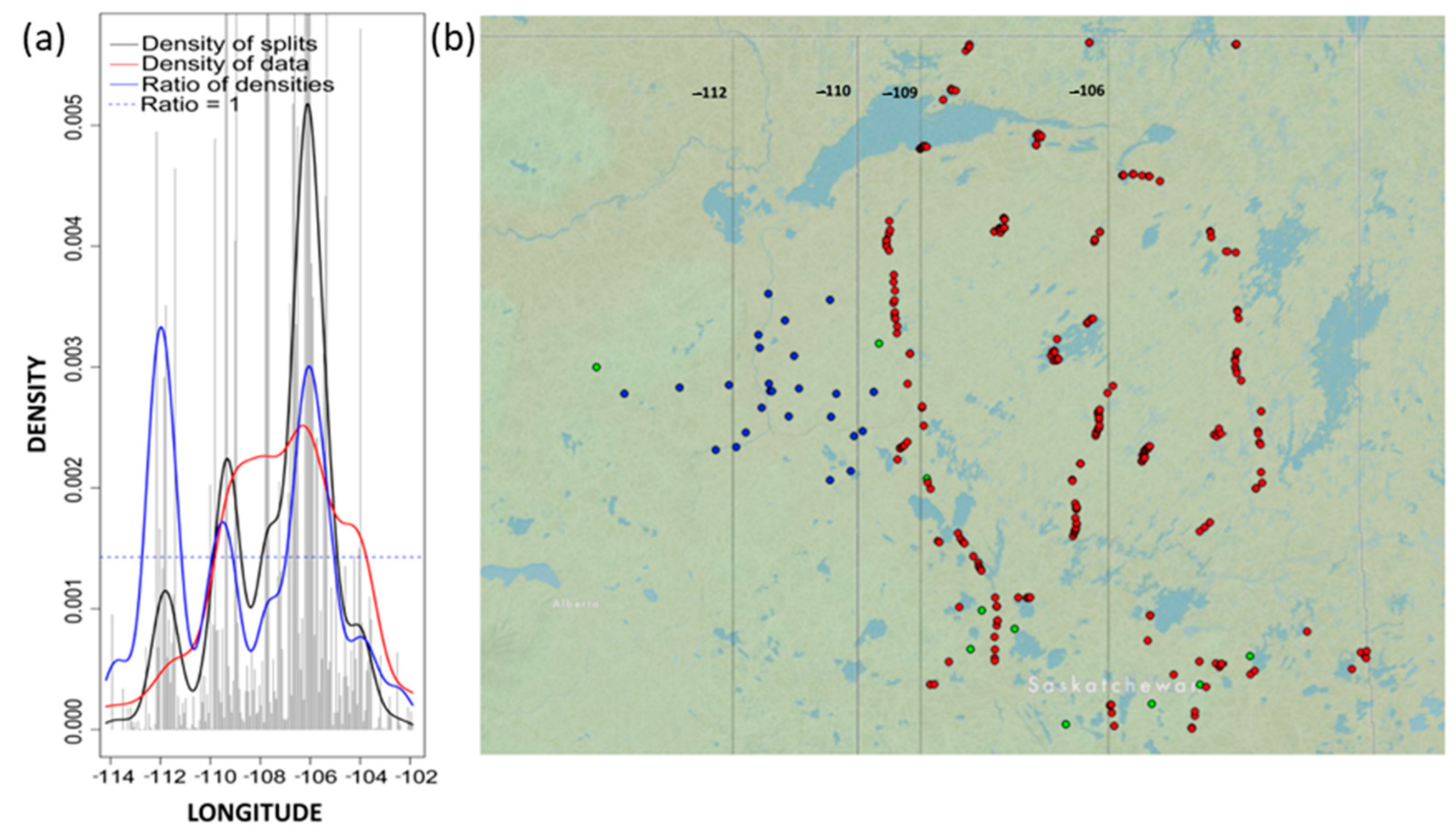
In addition to longitude, which remained the most important environmental variable (R2 = 0.0161, Table 4), both latitude and elevation were also identified as important predictors (Figure 3 and Table 4). The densities plot produced in gradient forest revealed that important splits (changes in abundance) occurring around −112 and around −106 (Figure 4) appeared to be consistent with different sampling efforts outlined across the WBEA, SK-FEC, and NFI survey protocols. The longitude densities plot also revealed an important split between −109 and −110 (Figure 4), consistent with the provincial boundary of Alberta and Saskatchewan, again outlining the variations in sampling efforts per survey and province.
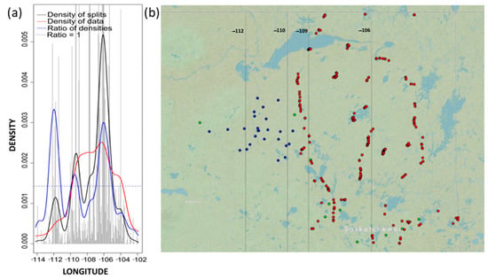
Figure 4.
(a) Densities plot for longitude with binned split importance values (grey histogram bars), the density of data (red line), the density of splits (black line), the ratio of split-over-density (blue line). The dashed line is where the ratio = 1. Relatively greater community level changes (high split importance values) occur when the ratio of densities > 1; and (b) map of study sites across Alberta and Saskatchewan (n = 297), with vertical black lines indicating longitude values where gradien forest identified thresholds.
Six deposition variables (in weighting order: HSO3, DNO, TDS, DSO2, DNO2 and DHNO, Figure 3 and Table 4) were among the top 15 variables with greatest R2-weighted importance. Among these variables, five were also identified as having high accuracy importance values, with only dry nitroxyl having a much lower comparative value (Figure 3), indicating very low predictive power. The remaining variables among the top 15 with greatest R2-weighted importance values were longitude, latitude, elevation and six bioclimatic variables. Only longitude, latitude and two bioclimatic variables, including Gdd above base temperature for period 2 (sg_09) and annual mean temperature (sg_12), had a relatively high associated accuracy importance value (Figure 3). Although these variables had high overall conditional importance (high values for both accuracy importance and R2-weighted importance), they are widely documented abiotic drivers for species distribution and were excluded from further analysis [51]. The remaining four bioclimatic variables had relatively low accuracy importance values, including total precipitation for period 1 (sg_04), precipitation of the driest quarter (bio_17), precipitation of the coldest quarter (bio_19), and annual minimum temperature (sg_13), and were excluded from further review as they were identified as having very little predictive power across the model (Figure 3).
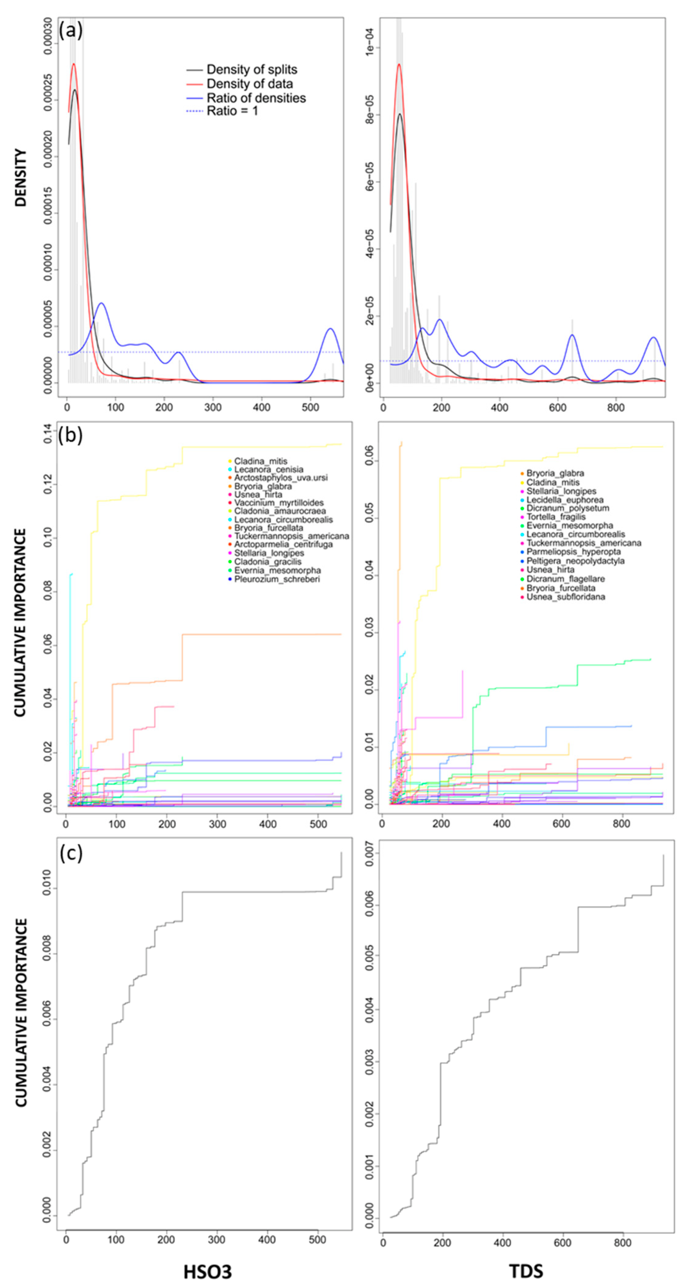
Wet hydrogen sulfite was an important environmental variable with respect to changes in community-level composition. The associated densities plot revealed two important community thresholds (where the ratio of densities > 1, Figure 5, left column), with the first threshold occurring between 70 and 80 eq ha−1 yr−1 and the second at 550 eq ha−1 yr−1 (Figure 5). Both peaks were relatively small but the first was representative of a slightly more significant community threshold. In addition, the secondary peak not only had a small ratio of densities (Figure 5), indicating that very little is occurring at the community level, but this peak was also located at the extremity of the gradient, representing a possible bias in the data [50]. The cumulative importance plots revealed several species experiencing smaller changes across the first range, including Stellaria longipes and Arctoparmelia centrifuga, but the species experiencing the most substantial change was Cladina mitis (Figure 5). Across the wet hydrogen sulfite gradient, the specific R2 performance value (R2S, Table 3) was greatest for Cladina mitis, indicating that wet hydrogen sulfite explained the greatest amount of variation within this species.
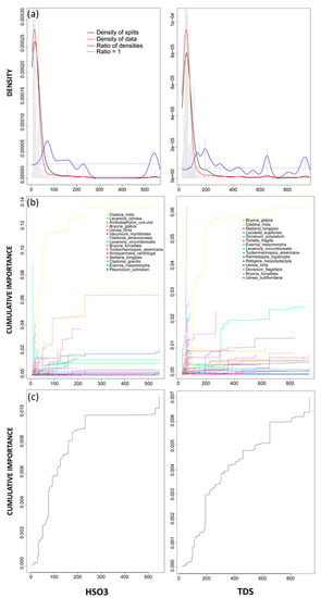
Figure 5.
(left column) gradient forest results for HSO3 and (right column) TDS. (a) Densities plot with binned split importance values (grey histogram bars), the density of data (red line), the density of splits (black line), the ratio of split-over-density (blue line). The dashed line is where the ratio = 1. Relatively greater community level changes (high split importance values) occur when the ratio of densities > 1; (b) species cumulative importance plot showing the cumulative distribution of splits importance scaled by R2. Each line represents an individual species, and the legend identifies the top 15 species experiencing the largest composition changes across the gradient; and (c) community cumulative importance plots calculated by the sum of weighted averages of all species in (b) and showing the overall pattern of compositional change for all species.
As the 8th most important predictor (R2-weighted importance) and high accuracy importance (Figure 3), TDS was also an important variable in the gradient forest model. The densities plot for TDS identified several community thresholds across the gradient, with the greatest ratio of densities peak (ratio of densities > 1) occurring between 150 and 200 eq ha−1 yr−1 (Figure 5, right column). Additional smaller peaks occurred around 650 eq ha−1 yr−1 and between 900–950 eq ha−1 yr−1 (Figure 5). Similar to wet hydrogen sulfite, the secondary, smaller thresholds have low density of data (red line) and low density of splits, indicating that very little is occurring at the community level (Figure 5). The cumulative importance plot for TDS identified Cladina mitis and Peltigera neopolydactyl as species experiencing the most change across this threshold (Figure 5). Several species, including Bryoria glabra, Stellaria longipes and Dicranum flagellare experienced substantial changes on an individual species level but these did not contribute to any important community level thresholds (Figure 5). However, across the full gradient, TDS explained the greatest amount of variation for Bryoria glabra (highest specific R2S performance value returned by gradient forest; Table 3). When wet hydrogen sulfite and TDS were compared, there was a high correlation factor found between both gradients (0.94), with the first threshold across the wet hydrogen sulfite gradient (70–80 eq ha−1 yr−1) correlating well with the 150–200 eq ha−1 yr−1 threshold across the TDS gradient.
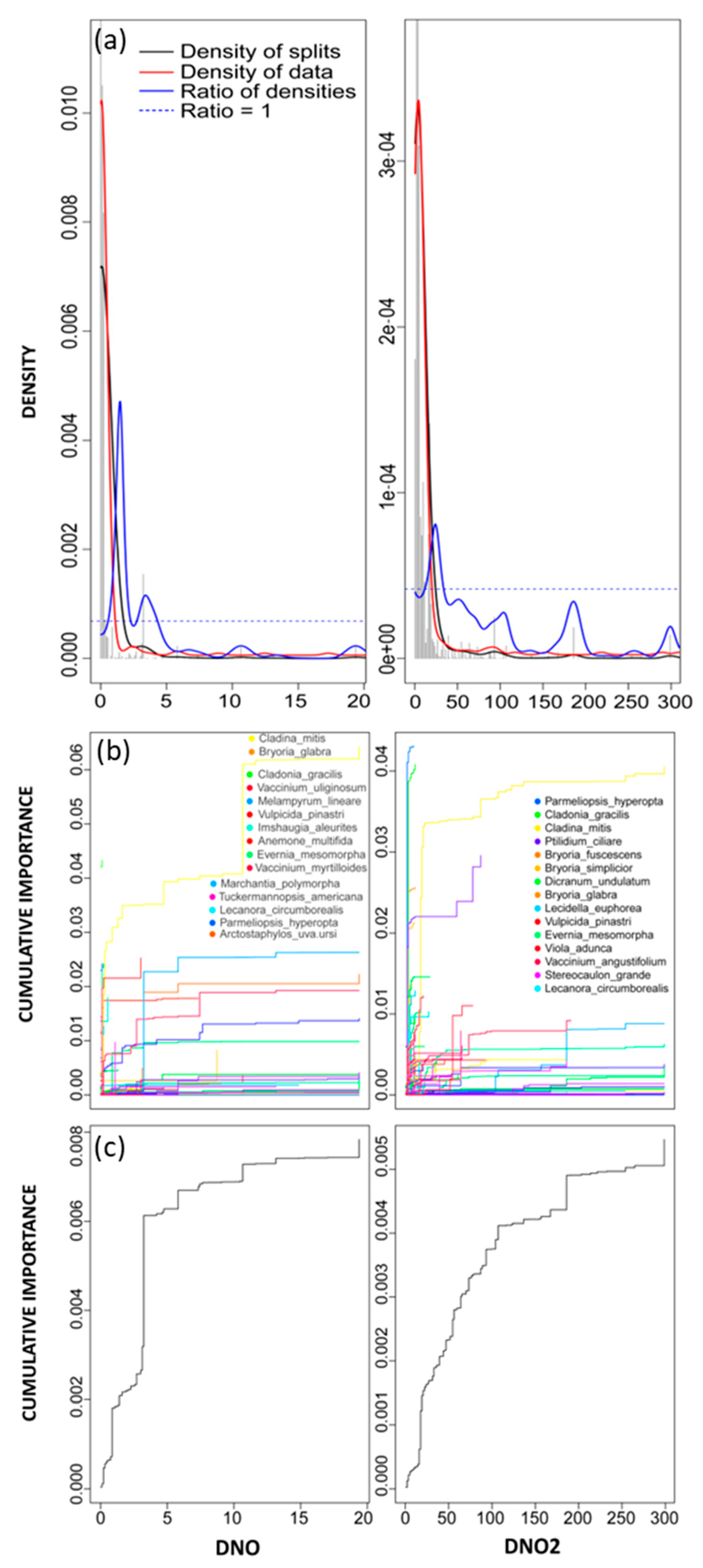
Dry nitrogen oxide and DNO2 had relatively high R2-weighted importance and accuracy importance (4th and 13th most important variable, respectively, Figure 3). The associated densities plots revealed that a large proportion of species’ abundance breakpoints (denoted by grey histogram bars) were relegated to low levels of deposition (Figure 6, left column). The densities plot for DNO identified two thresholds, the first located between 1 and 2 eq ha−1 yr−1 and the second located between 3 and 4 eq ha−1 yr−1, with greater binned split importance and a much greater ratio of densities associated to the first peak (Figure 6). The densities plot for DNO2 revealed a single threshold (where the ratio of densities was > 1 and binned split importance values peaked, Figure 6, right column) that ranged between 10 and 40 eq ha−1 yr−1 and peaked around 25 eq ha−1 yr−1.
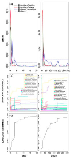
Figure 6.
Gradient forest results for DNO (left column) and DNO2 (right column). (a) Densities plot with binned split importance values (grey histogram bars), the density of data (red line), the density of splits (black line), the ratio of split-over-density (blue line). The dashed line is where the ratio = 1. Relatively greater community level changes (high split importance values) occur when the ratio of densities > 1; (b) species cumulative importance plot showing the cumulative distribution of splits importance scaled by R2. Each line represents an individual species, and the legend identifies the top 15 species experiencing the largest composition changes across the gradient; and (c) community cumulative importance plots calculated by the sum of weighted averages of all species in (b) and showing the overall pattern of compositional change for all species.
Although these are quite low levels of deposition, the cumulative importance plots for DNO and DNO2 revealed several reoccurring species that experienced substantial changes across identified thresholds including Cladina mitis, Bryoria glabra, Cladonia gracillis, Vulpicida pinastri, and Lecanora circumborealis. For DNO, individual species changes were greatest for Cladina mitis, Tuckermanopsis americana, and Evernia mesomorpha across the first, more pronounced community level threshold (Figure 6). Species associated with the secondary threshold, including Melampyrum lineare, Bryoria glabra, and Vaccinium uliginosum, experienced large cumulative changes at the individual species level but did not result in a large community threshold (Figure 6). It should be noted that across the entire DNO gradient, Cladina mitis had the greatest specific R2 performance value (R2S, Table 3), indicating that DNO explained the most amount of variation across this individual species. The cumulative importance plot for DNO2 revealed individual species changes that were more pronounced for Cladina mitis and Vulpicida pinastri at the peak of the ratio of densities curve (Figure 6). Several other species experienced large cumulative importance changes across this gradient but did not contribute to an overall community level threshold. The greatest specific R2 performance value across the DNO2 gradient belonged to Parmeliopsis hyperopta, indicating that variance for the entire species was best explained by DNO2.
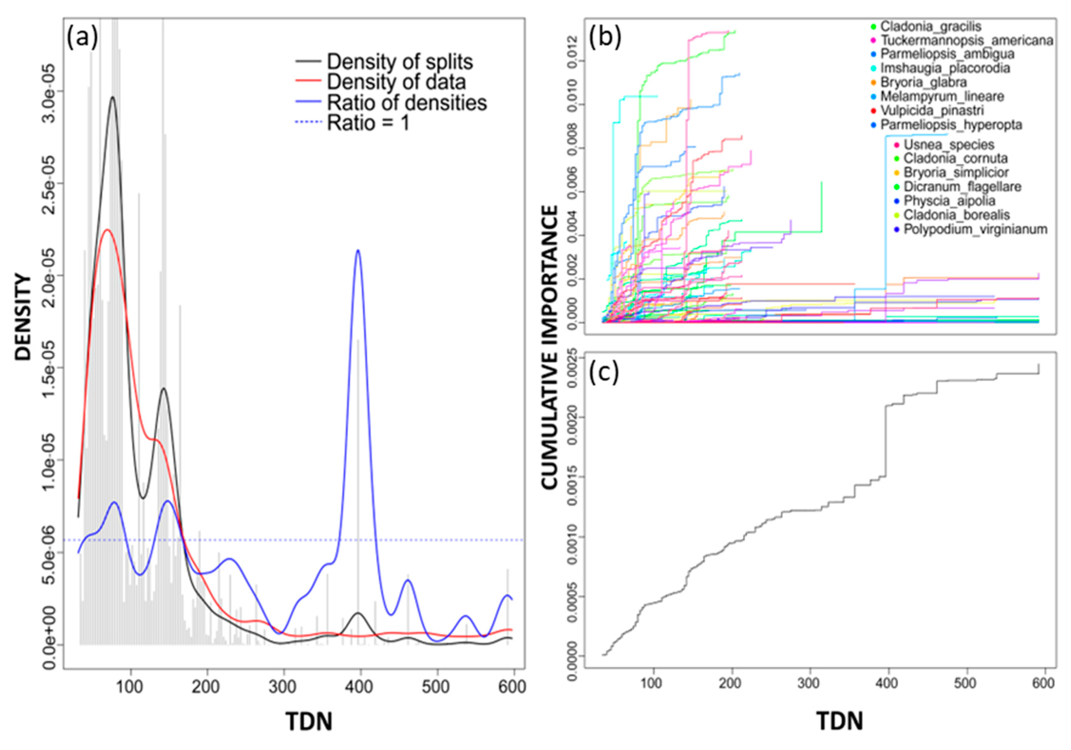
The densities plot for TDN revealed a high density of data between 0 and 200 eq ha−1 yr−1 (red lines, Figure 7). Binned split importance values also peaked in this range and the ratio of densities showed two minor thresholds in this region (around 80 eq ha−1 yr−1 and again around 150 eq ha−1 yr−1, Figure 7), indicating that compositional change is occurring, but the resulting overall community-level change is minor. A more pronounced community threshold was present around 400 eq ha−1 yr−1. However, both R2-weighted importance and mean accuracy importance values were very low for TDN, as such TDN breakpoints might not represent a reliable community threshold. Instead, a TDN threshold was inferred by evaluating the correlation between N deposition variables. Variables with relatively high correlation coefficients were considered and a TDN threshold was estimated by evaluating the equivalent TDN value or range from the line of best fit and the corresponding gradient forest threshold value or range of the correlated variable.
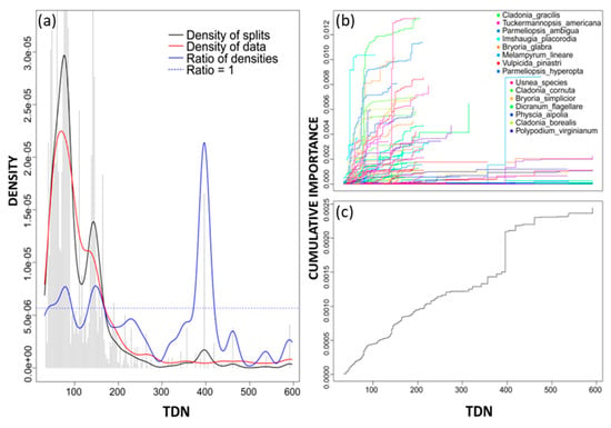
Figure 7.
(a) Densities plot for TDN with binned split importance values (grey histogram bars), the density of data (red line), the density of splits (black line), the ratio of split-over-density (blue line). The dashed line is where the ratio = 1. Relatively greater community level changes (high split importance values) occur when the ratio of densities > 1; (b) species cumulative importance plot showing the cumulative distribution of splits importance scaled by R2. Each line represents an individual species, and the legend identifies the top 15 species experiencing the largest composition changes across the gradient; and (c) community cumulative importance plots calculated by the sum of weighted averages of all species in (b) and showing the overall pattern of compositional change for all species.
The correlation coefficients for DNO and DNO2 (both identified as important predictors in gradient forest) were 0.586 and 0.735, respectively. Community thresholds for DNO (between 1 and 2 eq ha−1 yr−1) and DNO2 (around 25 eq ha−1 yr−1) were evaluated and resulted in TDN equivalents around 100 eq ha−1 yr−1 and 150 eq ha−1 yr−1, respectively. While DNH3 had the greatest correlation coefficient (0.904, Table 5) and relatively high mean accuracy importance, it was identified as having only intermediate importance (24th for variable importance, Figure 3). Therefore, TDN threshold values or ranges inferred from DNH3 were not considered as they might not be truly representative of community level changes. Based on results from gradient forest and correlation evaluations, it is reasonable to infer that community thresholds in the study area were between 100 to 150 eq ha−1 yr−1 for TDN, and between 150 and 200 eq ha−1 yr−1 for TDS.

Table 5.
Nitrogen deposition variables evaluated for correlation. Highly correlated gradient forest thresholds were used to infer TDN thresholds.
4. Discussion
4.1. Drivers of Community Thresholds
Overall, gradient forest analysis revealed that the variables with greatest predictor importance were predominantly bioclimatic variables (Figure 3). Given the large area covered by our study sites, and therefore the wide range in environmental variables, it would make sense that community thresholds seen in gradient forest were driven more by regional and climatic variables. This has been seen in other studies, where there was less of an effect of deposition on plant species composition when spatial scale was increased [51,52,54,55].
Gradient forest identified several deposition variables with high R2-weighted importance and accuracy importance, indicating that despite the broad spatial scale of our study, atmospheric deposition remained an important factor with respect to changing community composition. Similarly, in Switzerland, elevated N deposition has been shown to contribute, albeit minimally, to changes in plant species community composition across a large spatial scale [56]. Total sulphur deposition and wet hydrogen sulfite were identified as deposition variables with high predictor importance (Figure 3). While wet hydrogen sulfite had the greatest predictor importance of all deposition variables, it also accounted for approximately 30% of TDS. Gradient forest returned community thresholds for wet hydrogen sulfite between 70–80 eq ha−1 yr−1 and around 200 eq ha−1 yr−1 for TDS (equivalent to approximately 3.2 kg S ha−1 yr−1). While TDS was an important predictor with respect to plant species community composition, only 4% of all 297 study sites received TDS levels greater than the estimated community threshold, indicating that TDS induced changes occurring at the plant species community level might be relatively localized across only a small portion of sites.
In contrast, 15% of all 297 sites received TDN greater than the estimated community threshold. While modelled DNO was not a large overall contributor to TDN, gradient forest results still identified DNO and DNO2, both oxidized forms of N, as important predictors with respect to plant species community composition. Several studies have shown that both individual plant species and entire ecosystems can have varying sensitivity to different forms of N deposition, documenting in some cases greater sensitivity to reduced N deposition [54,57,58,59] and in other cases to oxidized N [60,61]. However, as seen in our study, DNO is known to contribute a relatively small amount to total dry deposition in North America [62] and the thresholds identified by gradient forest for DNO and DNO2 independently are very low. Rather, the importance of DNO and DNO2 seen in gradient forest could be the result of variability in the modelled deposition data. Although modelled deposition estimates were reasonable compared to actual deposition data, there was a low bias in N deposition estimates that required model correction [45]. While our results could be an ecosystem response indicating a preference to oxidized forms in Jack pine dominant forests, the interacting effects of deposition with other factors, including light availability or soil fertility [63] may also be partly responsible for the increased importance of oxidized over reduced N in our study area. Alternatively, it could also indicate that modelled TDN may not be fully reliable or that variables contributing to TDN, including DNO or DNO2, were better represented in the model.
Thresholds identified for the top deposition predictors were highly variable. Dry nitrogen dioxide had a single community threshold around 25 eq ha−1 yr−1 (Figure 6), and it represented almost 30% of TDN. In contrast, important community thresholds for DNO were identified at relatively low deposition levels (between 1–2 eq ha−1 yr−1 and 2.5–4 eq ha−1 yr−1, Figure 6), and DNO only accounted for 1.3% of TDN. Although gradient forest analysis determined that at a regional scale, total modelled N deposition was a smaller contributor to changes in plant species community composition than either DNO or DNO2, these predictors were relatively well correlated to TDN (Table 5) and inferred a threshold range for TDN between 100–150 eq ha−1 yr−1, equivalent to approximately 1.4 to 2.1 kg N ha−1 yr−1.
Our study revealed a lower N threshold compared to some studies; however, these studies often used a variety of species metrics, including species richness or species diversity to assess community changes [30,56,64,65]. In other studies, changes in ecosystem function or mechanisms were used to derive empirical critical loads of N. For instance, across similar European woodlands and forested habitats, a range of 5–15 kg N ha−1 yr−1 was recommended based on several indicators of exceedance, including changes in soil processes, nutrient imbalances, and changes in species composition across ground vegetation [23]. In this same study, they also found that declines in lichen, specifically, were associated with N deposition as low as 5–10 kg ha−1 yr−1 [23]. More recently, there has been a notable shift in deriving critical loads with greater emphasis placed on observed changes across specific taxa or individual species rather than using broad species metrics. For lichen communities across northern hardwood and coniferous forests in the United States, a range of 1–9 kg N ha−1 yr−1 was recommended [20], while a critical load of 1.5 kg N ha−1 yr−1 was estimated specifically for lichen communities in the Northwestern US [66]. These biodiversity-based critical loads, specific to lichen communities, are similar to this study.
4.2. Species & Community Level Response
Species cumulative importance curves for N-related predictors with high importance (DNO and DNO2, Figure 6) revealed several similarities in species response. Species that were most highly associated with the only threshold across the DNO2 gradient (25 eq ha−1 yr−1, Figure 6), were predominantly lichen, including Cladina mitis, Vulpicida pinastri, Evernia mesomorpha, and Lecanora circumborealis (Figure 6). These same lichen species were also identified as highly responsive across the primary threshold (1–2 eq ha−1 yr−1) along the DNO gradient (Figure 6). In addition, all but Vulpicida pinastri were found to be particularly well predicted by all environmental variables used in the model (R2 > 0.4, Figure 2). This is indicative that not only were DNO and DNO2 important drivers of changepoints for these species, but that these changepoints were also significant with respect to community-level change. In addition to being among the most responsive species in the model, our study also found that for N-related predictors, several lichens, including Cladina mitis and Evernia mesomoprha experienced changepoints at relatively low deposition levels. Other studies evaluating species-specific responses have identified similar lichen as bioindicators to changing environmental conditions [20,67,68]. For instance, in Sweden, three years of fertilization (at 150 kg N ha−1 or more) resulted in a marked reduction in cover for Cladina species in boreal forests [69]. While in a separate study, the effects of a five-year liquid fertilization treatment found that high abundance lichen, particularly Cladina species, disappeared entirely from the bottom layer vegetation [70]. Although these studies were carried out in boreal forests across Europe, the habitats are analogous to Jack pine stands in the boreal forests of Canada [15] and previous studies and reviews have identified similar N sensitivities for lichen communities [68,71,72].
It has been well documented that lichen respond primarily to air concentrations for N [73], which could explain why both DNO and DNO2 were among the top drivers of changes in lichen composition across the gradient forest model, out-performing TDN as a driver of species change. Increased lichen sensitivity to increased N emissions in aerosol form is predicated on their physiology. While vascular plants have specialized tissues that regulate the entry of gases, lichen do not, and instead will rapidly absorb gases, water, and dissolved nutrients, including increased N in the region [20,23,74]. Overall, increased atmospheric deposition can result in a shift in species composition when existing species in the area absorb more N than nutritionally required [73]. When they can no longer process any excess N, more N-tolerant, nitrophilous species begin to replace them, a well-documented response to increased N deposition [20,23,73,75,76].
The importance of lichen was well captured in gradient forest analysis with nine of 13 species that were particularly well predicted (by all 43 environmental variables) being lichen (R2 > 0.4, Figure 2, Table 3). However, vascular species, which represented the remaining four of 13 species that were well predicted by gradient forest, were also relevant to the model (R2 > 0.4, Figure 2). A closer look at the individual predictors responsible for change across top responding vascular species revealed that, apart from bioclimatic predictors, DNO was a recurring driver (Table 3). In addition, a secondary threshold across the DNO gradient (between 2.5–4 eq ha−1 yr−1, Figure 6) revealed several vascular species that exhibited important changes in this range. In response to N deposition, changes in competitive relationships can alter vascular communities [77]. While fast-growing grasses, sedges, and herbs will often experience an increase in cover, slow-growing, ericaceous shrubs often experience a decline in cover [10,77,78]. Vascular plants experiencing significant change across the secondary threshold for DNO included Arctostaphylos uva-ursi, Vaccinium uliginosum, Vaccinium myrtilloides, Melampyrum lineare, and Elymus innovatus, a grass (Figure 6). Several of these species are commonly found across the boreal forest and the response, particularly for Arctostaphylos uva-ursi or Vaccinium species, is consistent with findings from previous studies noting a decline in abundance in response to N addition [77,78,79,80]. In a study of heathlands across Britain, a negative relationship was observed between Arctostaphylos uva–ursi and modelled N deposition greater than 15 kg N [28]. However, in a study of boreal forests in Sweden, abundance of several Vaccinium species was associated to N deposition greater than 6 kg N ha−1 yr−1 [77]. These results are similar to our study, where the secondary DNO threshold, which correlated to approximately 2.45–3.15 kg N ha−1 yr−1 on the TDN gradient, revealed that change for many vascular species was occurring at the low end of (or lower than) the recommend critical load range of 3–15 kg N ha−1 yr−1 [24].
4.3. Uncertainties & Limitations
In our study, one of the more evident limitations was combining data from multiple surveys, as sampling efforts were not consistent among them. We attempted to reduce background variability by specifically selecting Jack pine dominant forests for analysis, however given the broad spatial scale in addition to data being compiled from observations by different surveyors across different surveys, we were not able to reduce variability indefinitely. Furthermore, the mean R2-weighted importance identified in gradient forest was relatively low (Table 4), indicating that the combination of all environmental variables explained a considerably small amount of overall variation. While this could be associated to uncertainties regarding how well the scale of our modelled deposition data were able to capture variation in the model, a low mean R2 is not necessarily out of the ordinary for gradient forest analysis. In a review of previous studies using gradient forest methodology [47], overall explainable variation was often relatively low, but this was attributed to the selection of predictor variables used in each analysis. In this study, it is possible that including more defined site descriptors, including soil data, could increase the amount of total explained variation [50]. However, it has been recognized that environmental variables alone cannot explain all changes associated with plant species composition or community thresholds across a gradient and a truly comprehensive dataset would also include variables such as historical events, including fire history, species interactions, and even temporal variability [47].
Gradient forest does not indicate a direction associated with the identified community or species thresholds. As such, careful analysis of both community and independent species thresholds is often required, along with additional information relating to a given ecosystem or study area to determine whether a threshold is presently associated with ecological degradation or restoration [50]. In addition, because gradient forest relies on a minimum number of species occurrences across a survey to determine a community threshold, rare species can be overlooked. In this study, a minimum of three occurrences was required per species, but even increasing this to seven [50] may still result in overlooking rare species that might be ecologically relevant.
Despite these limitations, gradient forest proved to be beneficial for several reasons with respect to this dataset. Similar to TITAN, gradient forest has a multivariate analysis approach that can account for most species in a survey and assumes that each species could represent a possible indicator for one of the environmental variables [38]. In addition, gradient forest, which is predisposed to produce a stair-step-like response rather than a linear response, is adept at modelling abundance data, which can often be sparse and discontinuous across a large survey [38]. However, the greatest asset for gradient forest is its ability to account for multiple environmental variables at once and in turn produce community threshold information using a singular unit (R2) that can be compared across all gradients [36,38,48,50].
5. Conclusions
In this study, community thresholds were predominantly associated with specific plant species that were well predicted by the gradient forest model and previously identified as indicators of N addition, including Cladina mitis, Evernia mesomoprha, and Arctostaphylos uva-ursi. Our analysis inferred two distinct community thresholds across the total nitrogen deposition gradient. The primary threshold ranged from 1.4 to 2.1 kg N ha−1 yr−1 and was predominantly associated with changes in lichen species. The secondary threshold, between 2.45 and 3.15 kg N ha−1 yr−1, suggested changes occurring across vascular species that are known bioindicators of increased N deposition. Additional work emphasizing the species-specific response to N deposition, particularly for species such as Arctostaphylos uva-ursi and Vaccinium species in similar habitats, could be beneficial in further characterizing this relationship. Given the two thresholds, we recommend a biodiversity-based empirical critical load for nutrient N of 1.4 to 3.15 kg N ha−1 yr−1 across Jack pine forests in northwestern Canada.
Supplementary Materials
The following supporting information is available online at https://www.mdpi.com/article/10.3390/nitrogen4010008/s1, SM I: Vegetation plot configurations and survey information, SM II: Gradient forest Information, SM III: Gradient forest density and species cumulative importance plots.
Author Contributions
Conceptualization, N.V. and J.A.; methodology, N.V. and J.A.; formal analysis, N.V.; investigation, N.V.; writing—original draft preparation, N.V. and J.A.; writing—review and editing, N.V. and J.A.; funding acquisition, J.A. All authors have read and agreed to the published version of the manuscript.
Funding
This project was carried out with financial support from Environment and Climate Change Canada (G&C GCXE19S022).
Data Availability Statement
Data used in this study are provided in the Supplementary Materials.
Acknowledgments
We gratefully acknowledge the contributions of Kevin Adkinson, Scott Baker, Phaedra Cowden, Jeremy Dunham, and Tanner Liang with field work and laboratory analysis. Moreover, we thank Hazel Cathcart, Morgan Kleiber, and Kayla Wilkins for their assistance in statistical computing and programming.
Conflicts of Interest
The authors declare no conflict of interest.
References
- Aber, J.D.; Nadelhoffer, K.J.; Steudler, P.; Melillo, J.M. Nitrogen saturation in northern forest ecosystems. BioScience 1989, 39, 378–386. [Google Scholar] [CrossRef]
- Fenn, M.E.; Haeuber, R.; Tonnesen, G.S.; Baron, J.S.; Grossman-Clarke, S.; Hope, D.; Jaffe, D.A.; Copeland, S.; Geiser, L.; Rueth, H.M.; et al. Nitrogen emissions, deposition and monitoring in the Western United States. Bioscience 2003, 53, 391–403. [Google Scholar] [CrossRef]
- Galloway, J.N.; Aber, J.D.; Erisman, J.W.; Seitzinger, S.P.; Howarth, R.W.; Cowling, E.B.; Cosby, B.J. The nitrogen cascade. Bioscience 2003, 53, 341–356. [Google Scholar] [CrossRef]
- Environment and Climate Change Canada. Canadian Environmental Sustainability Indicators: Air Pollutant Emissions. 2019. Available online: www.canada.ca/en/environment-climate-change/services/environmental-indicators/air-pollutant-emissions.html (accessed on 19 June 2019).
- Aherne, J.; Shaw, P. Impacts of sulphur and nitrogen deposition in western Canada. J. Limnol. 2010, 69, 1–3. [Google Scholar] [CrossRef]
- Bobbink, R.; Hornung, M.; Roelofs, J.G.M. The effects of air-borne nitrogen pollutants on species diversity in natural and semi-natural European vegetation. J. Ecol. 1998, 86, 717–738. [Google Scholar] [CrossRef]
- Dise, N.B.; Ashmore, M.; Belyazid, S.; Bleeker, A.; Bobbink, R.; de Vries, W.; Erisman, J.W.; Spranger, T.; Stevens, C.J.; van den Berg, L. Nitrogen as a threat to European terrestrial biodiversity. In The European Nitrogen Assessment; Sutton, M.A., Howard, C.M., Erisman, J.W., Billen, G., Bleeker, A., Grennfelt, P., van Grinsven, H., Grizzetti, B., Eds.; Cambridge University Press: Cambridge, UK; European Union: Brussels, Belgium, 2011; Chapter 20. [Google Scholar]
- Nordin, A.; Sheppard, L.; Strengbom, J.; Gunnarsson, U.; Hicks, K.; Sutton, M.A. Understanding of nitrogen deposition impacts: Topic 3. In Proceedings of the Background Document for the COST 729 Workshop on ‘Nitrogen Deposition and Natura 2000: Science and Practice in Determining Environmental Impacts’, Brussel, Belgium, 18–20 May 2009. [Google Scholar]
- Bobbink, R.; Ashmore, M.; Braun, S.; Flückiger, W.; Van den Wyngaert, I.J.J. Empirical nitrogen loads for natural and semi-natural ecosystems: 2002 update. In Empirical Critical Loads for Nitrogen, Environmental Documentation No. 164 Air; Achermann, B., Bobbink, R., Eds.; Swiss Agency for Environment, Forest and Landscape SAEFL: Berne, Switzerland, 2003. [Google Scholar]
- Bobbink, R.; Hicks, W.K. Factors affecting nitrogen deposition impacts on biodiversity: An overview. In Nitrogen Deposition, Critical Loads and Biodiversity; Sutton, M.A., Mason, K.E., Shepphard, L.H., Sverdrup, H., Haueber, R., Hicks, W.K., Eds.; Springer: Dordrecht, The Netherlands, 2014; Chapter 14; pp. 127–138. [Google Scholar]
- Duprè, C.; Stevens, C.J.; Ranke, T.; Bleekers, A.; Peppler-Lisbach, C.; Gowing, D.J.G.; Dise, N.B.; Dorland, E.; Bobbink, R.; Diekmann, M. Changes in species richness and composition in European acidic grasslands over the past 70 years: The contribution of cumulative atmospheric nitrogen deposition. Glob. Chang. Biol. 2010, 16, 344–357. [Google Scholar] [CrossRef]
- Köchy, M.; Wilson, S.D. Variation in nitrogen deposition and available soil nitrogen in a forest-grassland ecotone in Canada. Landsc. Ecol. 2004, 20, 191–202. [Google Scholar] [CrossRef][Green Version]
- Beaudoin, A.; Bernier, P.Y.; Villemaire, P.; Guindon, L.; Guo, X.J. Species Composition, Forest Properties and Land Cover Types across Canada’s Forests at 250m Resolution for 2001 and 2011; Natural Resources Canada, Canadian Forest Service, Laurentian Forestry Centre: Quebec, QC, Canada, 2017. [Google Scholar]
- ESRD: Environment and Sustainable Resource Development. Appendix I: Vegetation, wetlands and biodiversity. In Environmental Assessment—Cenovus TL ULC Telephone Lake In-Situ Project—EIA Report and Application for Approval; Volume 3 EIA–Appendices; Cenovus TL ULC & EnCana: Calgary, AB, Canada, 2011; Available online: https://open.alberta.ca/dataset/4871f71a-c541-47f5-9d79-58ef4a80851a/resource/c8f47757-8140-4e0e-9236-904eaae15f5d/download/v3appi.pdf (accessed on 15 February 2023).
- Allen, E.; Bayley, S.E. Effects of Nitrogen Deposition on Forests and Peatlands: A Literature Review and Discussion of the Potential Impacts of Nitrogen Deposition in the Alberta Oil Sands Region; Wood Buffalo Environmental Association: Fort McMurray, AB, Canada, 2007. [Google Scholar]
- Nilsson, J.; Grennfelt, P. Critical Loads for Sulphur and Nitrogen: Report from a Workshop Held at Skokloster, Sweden; UNECE and the Nordic Council of Ministers: Stockholm, Sweden, 1988. [Google Scholar]
- de Vries, W.; Hettelingh, J.-P.; Posch, M. Critical Loads and Dynamic Risk Assessments: Nitrogen, Acidity and Metals in Terrestrial and Aquatic Ecosystems; Environmental Pollution Series; Springer: Netherlands, Dordrecht, the Netherlands, 2015; Volume 25. [Google Scholar]
- Aherne, J.; Wilkins, K.; Cathcart, H. Nitrogen-Sulfur Critical Loads: Assessment of Impacts of Air Pollution on Habitats; EPA Research Report (2016-CCRP-MS.43); Environmental Protection Agency, Co.: Wexford, Ireland, 2021; 45p. [Google Scholar]
- Wilkins, K.; Clark, C.; Aherne, J. Ecological thresholds under atmospheric nitrogen deposition for 1200 herbaceous species and 24 communities across the United States. Glob. Chang. Biol. 2022, 28, 2381–2395. [Google Scholar] [CrossRef]
- Pardo, L.H.; Fenn, M.E.; Goodale, C.L.; Geiser, L.H.; Driscoll, C.T.; Allen, E.B.; Baron, J.S.; Bobbink, R.; Bowman, W.D.; Clark, C.M.; et al. Effects of nitrogen deposition and empirical nitrogen critical loads for ecoregions of the United States. Ecol. Appl. 2011, 21, 3049–3082. [Google Scholar] [CrossRef]
- Porter, E.; Blett, T.; Potter, D.U.; Huber, C. Protecting resources on federal lands: Implications of critical loads for atmospheric deposition of nitrogen and sulfur. BioScience 2005, 55, 603–612. [Google Scholar] [CrossRef]
- Bobbink, R.; Hicks, K.; Galloway, J.; Spranger, T.; Alkemade, R.; Ashmore, M.; da Cunha Bustamante, M.M.; Cinderby, S.; Davidson, E.A.; Dentener, F.; et al. Global assessment of nitrogen deposition effects on terrestrial plant diversity: A synthesis. Ecol. Appl. 2010, 20, 30–59. [Google Scholar] [CrossRef] [PubMed]
- Bobbink, R.; Hettelingh, J. Review and Revision of Empirical Critical Loads and Dose-Response Relationships: Proceedings of an Expert Workshop, Noordwijkerhout, 23–25 June 2010; Rijksinstituut voor Volksgezondheid en Milieu RIVM: Bilthoven, The Netherlands, 2011. [Google Scholar]
- Bobbink, R.; Loran, C.; Tomassen, H. Review and Revision of Empirical Critical Loads of Nitrogen for Europe; Texte 110/2022; German Environment Agency: Dessau-Roßlau, Germany, 2022; p. 358. [Google Scholar]
- Bobbink, R. Effects of Nutrient Enrichment in Dutch Chalk Grassland. J. Appl. Ecol. 1991, 28, 28–41. [Google Scholar] [CrossRef]
- Clark, C.M.; Tilman, D. Loss of plant species after chronic low-level nitrogen deposition to prairie grasslands. Nature 2008, 451, 712–715. [Google Scholar] [CrossRef]
- Pauli, D.; Peintinger, M.; Schmid, B. Nutrient enrichment in calcareous fens: Effects on plants species and community structure. Basic Appl. Ecol. 2002, 3, 255–266. [Google Scholar] [CrossRef]
- Henrys, P.A.; Stevens, C.J.; Smart, S.M.; Maskell, L.C.; Walker, K.J.; Preston, C.D.; Crowe, A.; Rowe, E.C.; Gowing, D.J.; Emmett, B.A. Impacts of nitrogen deposition on vascular plants in Britain: An analysis of two national observation networks. Biogeosciences 2011, 8, 3501–3518. [Google Scholar] [CrossRef]
- Roth, T.; Kohli, L.; Rihm, B.; Achermann, B. Nitrogen deposition is negatively related to species richness and species composition of vascular plants and bryophytes in Swiss mountain grassland. Agric. Ecosyst. Environ. 2013, 178, 121–126. [Google Scholar] [CrossRef]
- Maskell, L.C.; Smart, S.M.; Bullock, J.M.; Thompson, K.; Stevens, C.J. Nitrogen deposition causes widespread loss of species richness in British habitats. Glob. Chang. Biol. 2010, 16, 671–679. [Google Scholar] [CrossRef]
- Reinds, G.J.; Mol-Dijkstra, J.; Bonten, L.; Wamelink, W.; Hennekens, S.; Goedhart, P.; Posch, M. Probability of Plant Species (PROPS) Model: Latest Developments. In Modelling and Mapping the Impacts of Atmospheric Deposition of Nitrogen and Sulphur; Slootweg, J., Posch, M., Hettelingh, J.-P., Eds.; CCE Status Report 2015, RIVM Report 2015-0193; National Institute for Public Health and the Environment: Bilthoven, Netherlands, 2015; pp. 55–62. Available online: https://www.umweltbundesamt.de/sites/default/files/medien/4038/dokumente/2_cce_sr2015.pdf (accessed on 15 February 2023).
- Payne, R.J.; Dise, N.B.; Stevens, C.J.; Gowin, D.J.; BEGIN Partners. Impact of nitrogen deposition at the species level. Proc. Natl. Acad. Sci. USA 2013, 110, 984–987. [Google Scholar] [CrossRef]
- Wilkins, K.; Aherne, J.; Bleasdale, A. Vegetation community change points suggest that critical loads of nutrient nitrogen may be too high. Atmos. Environ. 2016, 146, 324–331. [Google Scholar] [CrossRef]
- Ellis, N.; Smith, S.J.; Pitcher, C.R. Gradient forests: Calculating importance gradients on physical predictors. Ecology 2012, 93, 156–168. [Google Scholar] [CrossRef]
- Breiman, L. Random Forests. Mach. Learn. 2001, 45, 5–32. [Google Scholar] [CrossRef]
- Pitcher, C.R.; Lawton, P.; Ellis, N.; Smith, S.J.; Incze, L.S.; Wei, C.-L.; Greenlaw, M.E.; Wolff, N.H.; Sameoto, J.A.; Snelgrove, P.V.R. Exploring the role of environmental variables in shaping patterns of seabed biodiversity composition in regional-scale ecosystems. J. Appl. Ecol. 2012, 49, 670–679. [Google Scholar] [CrossRef]
- Pitcher, C.R.; Ellis, N.; Smith, S.J. Example Analysis of Biodiversity Survey Data with R Package gradientForest. R Vignette. 2011. Available online: http://gradientforest.r-forge.r-project.org/biodiversity-survey.pdf (accessed on 15 February 2023).
- Roubeix, V.; Danis, P.-A.; Feret, T.; Baudoin, J.-M. Identification of ecological thresholds from variations in phytoplankton communities among lakes: Contribution to the definition of environmental standards. Environ. Monit. Assess. 2016, 188, 246. [Google Scholar] [CrossRef]
- ESWG: Ecological Stratification Working Group. A National Ecological Framework for Canada; Agriculture and Agri-Food Canada, Research Branch, Centre for Land and Biological Resources Research and Environment Canada, State of the Environment Directorate, Ecozone Analysis Branch: Ottawa/Hull, ON, Canada, 1995; p. 125. [Google Scholar]
- Wiken, E.B. Terrestrial ecozones of Canada. In Ecological Land Classification No. 19; Lands Directorate: Ottawa, ON, Canada, 1986; p. 26. [Google Scholar]
- Clair, T.A.; Percy, K.E. Assessing Forest Health in the Athabasca Oil Sands Region; WBEA Technical Report 2015-05-25; Wood Buffalo Environmental Association: Fort McMurray, AB, Canada, 2015; p. 180, + Appendices. [Google Scholar]
- McLaughlan, M.S.; Wright, R.A.; Jiricka, R.D. Field Guide to the Ecosites of Saskatchewan’s Provincial Forests; Saskatchewan Ministry of Environment, Forest Service: Prince Albert, SK, Canada, 2010; p. 343. [Google Scholar]
- Beaudoin, A.; Bernier, P.Y.; Villemaire, P.; Guindon, L.; Guo, X.J.; Bergeron, T.; Magnussen, S.; Hall, R.J. Mapping Attributes of Canada’s Forests at Moderate Resolution through kNN and MODIS Imagery. Can. J. For. Res. 2014, 44, 521–532. [Google Scholar] [CrossRef]
- CFIC: Canadian Forest Inventory Committee. Canada’s National Forest Inventory: Ground Sampling Guidelines; Natural Resources Canada, Canadian Forest Service, Pacific Forestry Centre: Victoria, BC, Canada, 2004. [Google Scholar]
- Makar, P.A.; Akingunola, A.; Aherne, J.; Cole, A.S.; Aklilu, Y.-A.; Zhang, J.; Wong, I.; Hayden, K.; Li, S.-M.; Kirk, J.; et al. Estimates of exceedances of critical loads for acidifying deposition in Alberta and Saskatchewan. Atmos. Chem. Phys. 2018, 18, 9897–9927. [Google Scholar] [CrossRef]
- McKenney, D.; Papadopol, P.; Campbell, K.; Lawrence, K.; Hutchinson, M. Spatial models of Canada- and North America-wide 1971–2000 minimum and maximum temperature, total precipitation and derived bioclimatic variables. In Frontline Forest Research Applications; Catalogue No. Fol23-1/106E-PDF; Minister of Supply and Services Canada: Sault Ste. Marie, ON, Canada, 2006. [Google Scholar]
- Compton, T.J.; Bowden, D.A.; Pitcher, C.R.; Hewitt, J.E.; Ellis, N. Biophysical patterns in benthic assemblage composition across contrasting continental margins off New Zealand. J. Biogeogr. 2012, 40, 75–89. [Google Scholar] [CrossRef]
- Large, S.I.; Fay, G.; Friedland, K.D.; Link, J.S. Quantifying patterns of change in marine ecosystem response to multiple pressures. PLoS ONE 2015, 10, e0119922. [Google Scholar] [CrossRef] [PubMed]
- Strobl, C.; Boulesteix, A.-L.; Kneib, T.; Augustin, T.; Zeileis, A. Conditional variable importance for random forests. BMC Bioinform. 2008, 9, 307. [Google Scholar] [CrossRef]
- Roubeix, V.; Daufresne, M.; Argillier, C.; Dublon, J.; Maire, A.; Nicolas, D.; Raymond, J.-C.; Danis, P.-A. Physico-chemical thresholds in the distribution of fish species among French lakes. Knowl. Manag. Aquat. Ecosyst. 2017, 418, 41. [Google Scholar] [CrossRef]
- Field, R.; Hawkins, B.A.; Cornell, H.V.; Currie, D.J.; Diniz-Filho, A.F.; Guegan, J.-F.; Kaufman, D.M.; Kerr, J.T.; Mittelbach, G.G.; Oberdorff, T.; et al. Spatial species-richness gradients across scales: A meta-analysis. J. Biogeogr. 2009, 36, 132–147. [Google Scholar] [CrossRef]
- Stevens, C.; Duprè, C.; Gaudnik, C.; Dorland, E.; Dise, N.; Gowing, D.; Bleeker, A.; Alard, D.; Bobbink, R.; Fowler, D.; et al. Changes in species composition of European acid grasslands observed along a gradient of nitrogen deposition. J. Veg. Sci. 2011, 22, 207–215. [Google Scholar] [CrossRef]
- Schleyer, M.; Porter, S. Drivers of soft and stony coral community distribution on the high-latitude coral reefs of South Africa. Adv. Mar. Biol. 2018, 80, 1–55. [Google Scholar] [CrossRef] [PubMed]
- Clark, C.M.; Phelan, J.; Doraiswamy, P.; Buckley, J.; Cajka, J.C.; Dennis, R.L.; Lynch, J.; Nolte, C.G.; Spero, T.L. Atmospheric deposition and exceedances of critical loads from 1800–2025 for the conterminous United States. Ecol. Appl. 2018, 28, 978–1002. [Google Scholar] [CrossRef]
- van Dobben, H.; de Vries, W. Relationship between forest vegetation, atmospheric deposition and site conditions at regional and European scales. Environ. Pollut. 2010, 158, 921–933. [Google Scholar] [CrossRef]
- Roth, T.; Kohli, L.; Rihm, B.; Amrhein, V.; Achermann, B. Nitrogen deposition and multi-dimensional plant diversity at the landscape scale. R. Soc. Open Sci. 2015, 2, 150017. [Google Scholar] [CrossRef]
- Dahlman, L.; Persson, J.; Palmqvist, K.; Näsholm, T. Organic and inorganic nitrogen uptake in lichens. Planta 2004, 219, 459–467. [Google Scholar] [CrossRef]
- Hogan, E.J.; Minnullina, G.; Sheppard, L.J.; Leith, I.D.; Crittenden, P.D. Response of phosphomonesterase activity in the lichen Cladonia portentosa to nitrogen and phosphorus enrichment in a field manipulation experiment. New Phytol. 2010, 186, 926–933. [Google Scholar] [CrossRef]
- Southon, G.E.; Field, C.; Caporn, S.J.M.; Britton, A.J.; Power, S.A. Nitrogen deposition reduces plant diversity and alters ecosystem functioning: Field-scale evidence from a nationwide survey of UK heathlands. PloS ONE 2013, 8, e59031. [Google Scholar] [CrossRef]
- Nordin, A.; Strengbom, J.; Ericson, L. Responses to ammonium and nitrate additions by boreal plants and their natural enemies. Environ. Pollut. 2006, 141, 167–174. [Google Scholar] [CrossRef] [PubMed]
- van den Berg, L.J.L.; Laurence, J.; Sheppard, L.J.; Smart, S.M.; Bobbink, R.; Dise, N.B.; Ashmore, M.R. Evidence for differential effects of reduced and oxidised nitrogen deposition on vegetation independent of nitrogen load. Environ. Pollut. 2016, 208, 890–897. [Google Scholar] [CrossRef] [PubMed]
- Kharol, S.K.; Shephard, M.W.; McLinden, C.A.; Zhang, L.; Sioris, C.E.; O’Brien, J.M.; Vet, R.; Cady-Pereira, K.E.; Hare, E.; Siemons, J.; et al. Dry deposition of reactive nitrogen from satellite observations of ammonia and nitrogen dioxide over North America. Geophys. Res. Lett. 2018, 45, 1157–1166. [Google Scholar] [CrossRef]
- Tulloss, E.M.; Cadenasso, M.L. The effect of nitrogen deposition on plant performance and community structure: Is it life stage specific? PLoS ONE 2015, 11, e0156685. [Google Scholar] [CrossRef] [PubMed]
- Stevens, C.J.; Dise, N.B.; Mountford, J.O.; Gowing, D.J. Impact of nitrogen deposition on the species richness of grasslands. Science 2004, 303, 1876–1879. [Google Scholar] [CrossRef]
- van den Berg, L.J.L.; Vergeer, P.; Rich, T.C.G.; Smart, S.M.; Guest, D.; Ashmore, M.R. Direct and indirect effects of nitrogen deposition on species composition change in calcareous grasslands. Glob. Chang. Biol. 2010, 17, 1871–1883. [Google Scholar] [CrossRef]
- Geiser, L.H.; Nelson, P.R.; Jovan, S.E.; Root, H.T.; Clark, C.M. Assessing ecological risks from atmospheric deposition of nitrogen and sulfur to US forests using epiphytic macrolichens. Diversity 2019, 11, 87. [Google Scholar] [CrossRef]
- Králikova, I.; Goga, M.; Bil’ová, I.; Bačkorová, M.; Bačkor, M. Response of lichens Cladonia arbuscula subsp. Mitis Cladonia Furcate Nitrogen Excess. Biol. 2016, 71, 632–638. [Google Scholar] [CrossRef]
- Thormann, M. Lichens as indicators of forest health in Canada. For. Chron. 2006, 82, 335–343. [Google Scholar] [CrossRef]
- Eriksson, O.; Raunistola, T. Impact of forest fertilizers on winter pastured of semi-domesticated reindeer. Rangifer 1991, 13, 203–214. [Google Scholar] [CrossRef]
- Kellner, O.; Marshagen, M. Effects of irrigation and fertilization on the ground vegetation of 130-year-old stand of Scots pine. Can. J. For. Res. 1991, 21, 733–738. [Google Scholar] [CrossRef]
- Fenn, M.E.; Bytnerowics, A.; Schilling, S.L.; Ross, C.S. Atmospheric deposition of nitrogen, sulfur and base cations in Jack pine in the Athabasca Oil Sands Region, Alberta, Canada. Environ. Pollut. 2015, 196, 497–510. [Google Scholar] [CrossRef]
- Laxton, D.L.; Watmough, S.A.; Aherne, J.; Straker, J. An assessment of nitrogen saturation in Pinus banksiana plots in the Athabasca Oil sands Region, Alberta. J. Limnol. 2010, 69, 171–180. [Google Scholar] [CrossRef]
- Carter, T.S.; Clark, C.M.; Fenn, M.E.; Jovan, S.; Perakis, S.S.; Riddell, J.; Schaberg, P.G.; Greaver, T.L.; Hastings, M.G. Mechanisms of nitrogen deposition effects on temperate forest lichens and trees. Ecosphere 2017, 8, e01717. [Google Scholar] [CrossRef]
- Hauck, M. Ammonium and nitrate tolerance in lichens. Environ. Pollut. 2010, 158, 1127–1133. [Google Scholar] [CrossRef] [PubMed]
- Fenn, M.E.; Baron, J.S.; Allen, E.B.; Rueth, H.M.; Nydick, K.R.; Geiser, L.; Bowman, W.D.; Sickman, J.O.; Neixner, T.; Johnson, D.W.; et al. Ecological effects of nitrogen deposition in the Western United States. Bioscience 2004, 53, 404–420. [Google Scholar] [CrossRef]
- Payne, R.J.; Dise, N.B.; Field, C.D.; Dore, A.J.; Caporn, S.J.M.; Stevens, C.J. Nitrogen deposition and plant biodiversity: Past, present, and future. Front. Ecol. Environ. 2017, 15, 431–436. [Google Scholar] [CrossRef]
- Prescott, C.E.; Kumi, J.W.; Weetman, G.F. Long-term effects of repeated N fertilization and straw application in a Jack pine forest. 2. Changes in the ericaceous ground vegetation. Can. J. For. Res. 1995, 25, 1984–1990. [Google Scholar] [CrossRef]
- Nordin, A.; Strengbom, J.; Witzell, J.; Näsholm, T.; Ericson, L. Nitrogen deposition and the biodiversity of boreal forests: Implications for the nitrogen critical load. Ambio A J. Hum. Environ. 2005, 34, 20–24. [Google Scholar] [CrossRef]
- Strengbom, J.; Walheim, M.; Näsholm, T.; Ericson, L. Regional differences in occurrence of understorey forest species reflects differences in N deposition in Swedish forests. Ambio 2003, 32, 91–97. [Google Scholar] [CrossRef]
- Turkington, R.; John, E.; Watson, S.; Seccombe-Hett, P. The effects of fertilization and herbivory on the herbaceous vegetation of the boreal forest in northwestern Canada: A 10-year study. J. Ecol. 2002, 90, 325–337. [Google Scholar] [CrossRef]
Disclaimer/Publisher’s Note: The statements, opinions and data contained in all publications are solely those of the individual author(s) and contributor(s) and not of MDPI and/or the editor(s). MDPI and/or the editor(s) disclaim responsibility for any injury to people or property resulting from any ideas, methods, instructions or products referred to in the content. |
© 2023 by the authors. Licensee MDPI, Basel, Switzerland. This article is an open access article distributed under the terms and conditions of the Creative Commons Attribution (CC BY) license (https://creativecommons.org/licenses/by/4.0/).

