1. Introduction
Precision agriculture seeks to extract relevant knowledge from various types of sensing information, in order to implement site-specific treatments for an efficient and sustainable management of crops. Such knowledge should allow improving the expected benefits for producers with respect to the already-existing practices and for the environment. In this way, data can be collected by sensors, continuously monitoring the condition of the field, and based on machine learning techniques, transforming the available information into relevant knowledge for intelligent decision-making.
Following the precision agriculture perspective, the management of the agricultural fields can be further improved to achieve greater gains or savings, by choosing the appropriate management zones for site-specific treatment. In this sense, this study is set out to test if by learning subareas in the field based on experimental local sensor readings, the expected costs of fertilisation can be minimised while ensuring the (post-harvest) levels of yield and quality obtained under a uniform approach. As a consequence, it should be noted that this application does not address the optimal fertilisation of the fields, but rather, it intends to show how soil and vegetation local sensors can aid the fertilisation decision process. Thus, it allows understanding the crop development and building a future decision support system that takes into account soil and vegetation real-time information.
Under this setting, management zones are understood as a group of parcels or plots, which are the experimental units that have been used for testing four different N-fertilisation treatments (consisting of one dose of 50 kg N/ha, from now on kg/ha, or repeated doses of up to 150, 200, and 300 kg/ha) on the yield and protein contents of winter wheat (Triticum aestivum) crops. The available data were collected from experimental sites at Kalundborg and Bjerringbro in Denmark.
In a first approach to the data, the effects of the fertilisation treatments are estimated, given the initial (experimental) parcelwise configuration. Then, after learning a new configuration for the management zones through unsupervised machine learning techniques, its impact is estimated by comparing the expected gains with respect to the uniform application, testing if a more sustainable use of resources can be achieved without negatively affecting the quality and quantity of the cereal production.
Revising the existing literature on learning management zones for precision agriculture, there has been a fair amount of studies related to clustering parcels due to soil and terrain properties for optimising yield [
1]. Regarding this issue, quadratic discriminant and k-nearest neighbour analysis were tested (see again [
1]), these being (supervised) classification techniques, examining the effectiveness of two such delineation procedures to identify yield temporal patterns from the specific site properties. That is, knowing the attributes of the field (as in any supervised learning task), the relation between yield and site attributes was verified, offering evidence for the relevance of studies developing unsupervised methodologies (like ours) to learn (sub-)optimal configurations of the field. These studies should allow achieving greater gains for the producers. Besides, it should be noted that our proposal not only considers yield, but also quality parameters such as the percentage of protein.
Considering different applications, one decision tool [
2] has been developed for zone mapping application, also estimating the optimal number of management zones. Such a tool uses satellite imagery and field data provided by users, learning the zones according to the natural variation of the soil organic matter and nutrients, reporting that their zone maps were quite similar to what is produced by traditional means. It should be noted that our methodology goes more into the micro-perspective, with (vegetation and soil) sensor readings being the main input, as the most basic system that can be implemented for fields trying to implement precision agriculture.
Another application can be found for geographical data [
3], where authors stress the strong connection between the challenges of precision agriculture with machine learning problems. More related to our approach, a cluster-based application [
4] has been proposed to identify management zones (for cotton production), focusing on both yield and field properties together with spatial information. This work uses only one clustering methodology, K-means, which is implemented looking at spatially contiguous zones (see also [
5]). As this work also addresses identifying an optimal number of management zones, it should be noted that our approach does not impose geographical adjacency, as our main focus consists of the automatic implementation of the methodology by sensor-based machine learning techniques.
Hence, we explore different types of clustering methods (both hierarchical-agglomerative and iterative) along with the corresponding stopping criteria, which allow evaluating how well the partition performs regarding its statistical properties. After the purely computational analysis, results are validated considering the case study for the wheat experimental fields.
In this sense, our approach addresses the automatic identification of the areas to be considered as site-specific management zones for the crops. Furthermore, our methodology is built on the optimisation of the resulting partition through clustering analysis, and it is validated with respect to the expected savings in fertilisation costs.
In this line of research, fuzzy K-means was applied to minimise the variability of cereal (wheat) crops, based on remote sensing information, vegetation, soil, and yield attributes [
6]. There, it was shown that the variance of the crop nutrients, wheat spectral parameters, and yield can be reduced under the proposed specification of the different zones. As their focus was mainly concentrated on the use of (satellite) remote sensing, our approach addresses only soil and vegetation local sensors. We acknowledge that this (sensor) information could be used together with other sources of information, including remote sensing and the observed or historical measurements of yield and crop nutrients (quality parameters), but aiming at developing a first
local precision system, we focus only on
sensor-based management zones and then validate its impact on yield and quality.
Most importantly, we stress that our study examines clustering analysis in detail, looking at the robustness of the solution from a statistical perspective. Therefore, we implemented different clustering methods according to a set of key information measures, optimising the statistical performance of the obtained partitions, which correspond to the proposed management zones, and validate the results according to the expected savings in fertiliser application. Besides, we propose a dissention degree among pairs of partitions, which allows us to measure how much any two zone configurations differ in terms of their cluster composition.
In order to do so, this paper is organised as follows. Firstly, the setting for collecting and analysing the experimental data is explained, together with the methodology for learning management zones. Then, in
Section 3, the results are presented and illustrated with the experimental crop data. In
Section 4, the methodology is validated and the results are discussed, assessing its impact on the producers’ expected gains/savings. The final
Section 5 ends with some conclusions and comments for future research.
2. Methodology
2.1. Sensor Data and Experimental Measurements on Yield and Quality
Two different experimental fields in Kalundborg and Bjerringbro, Denmark, were used during 2017 to study the effects of site-specific dosage on yield and protein attributes of wheat crops. Each field was randomly divided into a fixed number of parcels, 108 for Kalundborg and 52 for Bjerringbro, such that each parcel received a specific dose level of 50, 150, 200, and 300 kg/ha. Hence, there are four initial groupings for parcels according to the amounts of dosage (kg/ha) they received. Each parcel was 30 × 6 m, where each plot or parcel was harvested and weighed entirely.
For each parcel, data were collected by means of electrical in situ sensors, measuring the inherent characteristics of the crop by vegetation and soil electro-conductivity. Vegetation was measured by the N-sensor (
https://www.yara.us/, accessed on 9 May 2022), which offers an approximate crop status. The N-sensor scans 50 m
/s and measures light reflectance in the range from 450 to 900 nm. The N-sensor also has an upward sensor that measures irradiance in the same wavelength range as the downward sensor. The data outputs from the sensor were used in combination with an algorithm to give a relative biomass map and an N-rate map. Information on the specific wavelengths and algorithms used is not publicly available. In the current study, we used the relative biomass value for each plot as the input to our model. The N-sensor readings were made per plot, and the values were from 1.6 to 16.9 and are referred to as “YARA biomass readings” in
Table 1.
On the other hand, the soil electro-conductivity was measured by DualEM (
https://dualem.com/, accessed on 9 May 2022) instruments, which explore simultaneously different depths of the soil. For the vegetation measurements, four different readings were taken between March and June of 2017 (once per month), and for the soil readings, four different depths were considered, at 30, 60, 90, and 180 cm.
Additionally, post-harvest measurements were taken on the dry matter yield and protein of the cereal in the field. Dry matter yield was at 85% dry matter, and protein was measured using the combustion method, obtaining the total nitrogen and converting it to protein. In this way, all samples were ground through a 1 mm sieve and stored in small glass bottles (5.5 cm × 2.5 cm, height × diameter) before the subsequent measurement of the N concentration. Nitrogen concentration in the ground samples was measured using an elemental analyser (Vario EL III Germany), and N content in kg/ha was subsequently calculated by multiplying dry matter by N concentration.
2.2. Assessing Treatment Effects
Given a specific grouping of parcels according to the configuration of management zones, it is required to infer if there are significant effects of the amount of fertiliser dosage on the quantity and quality of the production. Then, after verifying the significance of the factor treatments, the effects that the different fertilisation strategies may have on dosage savings can be estimated.
Firstly, the initial dosage treatments were explored according to their effects on the yield and protein of the crop by the analysis of variance, that is measuring the deviation from the mean performance according to
where
is the response variable, in this case the observed amounts of yield, or the protein production levels, for each treatment
i and parcel
j. Here,
is the mean production or mean protein levels for all parcels,
stands for the
i-th (dosage) treatment effects, and
is the random error component, assuming it to have a normal distribution with zero mean and constant variance (for more details, see [
7]).
Then, a family of pairwise comparisons was developed on the dosage treatments for mean yield and protein levels (as in
Tukey [
8]), identifying the significant differences between them (while controlling the risk of rejecting the null hypothesis when in fact it should not be rejected). In this way, it is possible to select the best treatment under the initial experimental setting that minimises the use of fertiliser while achieving the same average yield or protein levels.
Regarding the impact of following different fertilisation strategies (referring to a uniform or a site-specific strategy), the potential savings on the fertilisation dosage can be roughly estimated by comparing the amounts of fertiliser that would be used under one setting (e.g., the experimental configuration) or another (e.g., a uniform dosage according to the Danish norm for winter wheat). Have in mind that this estimation assumes equivalent conditions of the fields where the different strategies were implemented.
Furthermore, if we take the Danish norm for winter wheat [
9], the uniform fertilisation would be given by
kg/ha at Kalundborg (due to its classification as a
clay type of soil) and by
kg/ha at Bjerringbro (being a
sandy clay type of soil). Therefore, it could be said that if a different setting allows achieving satisfactory mean levels of yield and quality while using less fertiliser, then this would entail greater savings and higher potential net benefits.
Besides the experimental setting, we would also like to explore if by learning a different configuration for
management zones, it would be possible to save on fertilisation costs. The methodology that we examine in the next
Section 2.3 will address the construction of new management zones for optimising the performance of the crops, and it will be validated against the uniform strategy. Then, its impact on decision-making can be assessed with respect to how much input of fertilisation could be saved if we applied a site-specific amount regarding the needs of each zone.
In this way, we take the mean amount of dosage for each (new) zone, computed over all parcels belonging to that zone, and measure the difference with respect to the uniform-norm treatment, checking if there are potential savings that can be achieved while ensuring desired levels of yield and quality.
Here, the mean expected fertilisation savings
are given by
where
K stands for the number of zones,
stands for the (uniform) amount received by each parcel under the Danish norm for winter wheat, and
stands for the mean dosage applied to all parcels belonging to the same zone.
Next, we present the methodology for learning management zones. Cluster analysis will be developed, aiming at answering the question of how many clusters allow obtaining a good partition.
2.3. Learning Management Zones by Cluster Analysis
The methodology of machine learning by clustering techniques was applied on the characteristic attributes for the agricultural parcels, consisting of the sensor data readings for soil and vegetation status. The techniques that were included in the analysis are hierarchical clustering (by forward agglomeration) and the iterative K-means, K-medoids, and fuzzy K-means. As will be discussed, each method has different construction principles, which allow obtaining heterogeneous partitions to find the one with the best statistical properties.
In general, clustering techniques allow searching for a particular structure in the data, based on evaluations of the similarity among the parcels. Here, the data that were used for building the clusters, which are regarded as the management zones, consisted of four readings for vegetation (taken at different points in time between March and May 2017) and four readings on soil conditions (taken at different depths). Hence, by applying different techniques and learning the best partition among parcels, the clusters or zones that better characterise the parcels can be properly identified.
2.3.1. Hierarchical Clustering
The methodology of hierarchical clustering that we explore here is agglomerative (as opposed to divisive), i.e., under the initial condition that each parcel is on its own, and the most proximal parcels are joined together under the same cluster until every parcel makes part of one final cluster. Hence, in the beginning of the process, clusters tend to be composed by very similar units, but as the process develops, the similarity threshold gets lower, allowing clusters to be composed of more dissimilar observations.
This technique (see, e.g., [
7]) allows building a tree-like hierarchical grouping, where the most proximal or similar parcels are sequentially grouped together. Therefore, under this approach, the similarity
between two clusters (
and
) is measured by the inverse of the distance function
, as in
Here, we take the Euclidean distance function, such that the distance between any pair of clusters is given by (
)
where
and
stand for the number of observations
and
in clusters
and
, respectively.
Regarding the linkage criterion for joining different clusters into a new cluster, we computed two types of partitions. They were built according to the minimum (maximum) distance, namely the
single linkage (
complete linkage) between the observations belonging to different clusters, in this way building different forms of groupings according to the way we compute the proximity between groups of observations. As an advantage of this methodology, it allows identifying clusters without a specific predefined shape, under two opposite linkage criteria (the single linkage, where the most proximal elements determine the configuration of the cluster, and the complete linkage, where proximity depends on the most distant elements), as the specific grouping depends on the chain of reasoning for (cluster) pairwise proximity. Nonetheless, this methodology still requires that the different clusters are well separated for a
good partition to be achieved, but having in mind that the means to properly assess the quality of a partition will be addressed in
Section 2.4.
2.3.2. K-Means Clustering
The clustering methodology of K-means partitions the set of parcels according to a given number K of different groups. An important requisite for implementing this algorithm is that the number of groups has to be previously established, so K can be set as a free parameter to be optimised with respect to the given clustering performance criteria.
The K-means procedure can be understood by a heuristic search of the
K best clusters that minimise the variability within the clusters. This problem is solved by finding the partition that minimises the within-cluster variability (see, e.g., [
10]):
where the variability is measured against the mean of the cluster. Hence, the
mean of a cluster
, with elements
, stands as the
prototype of that cluster.
In general, the K-means procedure obtains spherical clusters of comparable size, but it is highly sensitive to outliers, as the mean is easily influenced by extreme values. In this sense, a technique that is not as sensitive as K-means to outliers is used, namely K-medoids [
10], which is examined next.
2.3.3. K-Medoids Clustering
A variant of the K-means procedure allows building partitions that are more robust to noise and outliers. Instead of the mean, it uses a
medoid prototype, which refers to a real observation. Such a prototype is regarded as the most centrally located observation of the cluster, with the minimum sum of
dissimilarities to the other members of the cluster [
10].
The pairwise dissimilarities are computed by the absolute differences:
where
is the corresponding observation standing as the centroid prototype of the
g-th cluster.
2.3.4. Fuzzy K-Means Clustering
Among the different clustering techniques reviewed up to now, it is observed that the assignation of a parcel to a cluster follows a
hard or binary decision. That is, it belongs to just one specific cluster. Nonetheless, the frontiers between clusters are not always that clear, and in most cases, they have to be built under some degree of
uncertainty. This is recognised by different
soft methodologies, allowing each observation to belong to multiple clusters with different degrees of membership (see, e.g., [
10,
11], but also [
12]). Hence, the fuzzy K-means clustering algorithm is considered here [
13], where each element belongs to different clusters with different degrees of intensity.
In the same line as the iterative K-means and K-medoids, the fuzzy K-means partitions the data into a given number of
K clusters. Each cluster is represented by a prototype, which is as similar as possible to all the observations that are members of that cluster, obtained by minimising the function (see again [
13])
where
stands for the membership degree of observation
to cluster
,
is the distance function between
and the (simple) mean prototype of
, and the parameter
m represents the tolerance for cluster overlapping or how fuzzy the borders of clusters are allowed to be. That is, a higher value of
m allows a smoother transition form one cluster to another one than with smaller values (see, e.g., [
14]).
Then, under the restriction (
) that
the solution of the fuzzy K-means algorithm corresponds to
As a general rule, an observation is assigned to the cluster for which it has maximum membership intensity or to the cluster with minimal distance .
Taking the Euclidean distance (
4), it can be shown that the cluster prototypes
are given by
Besides, by setting the parameter , both K-means and fuzzy K-means obtain the same result, the former being a special case of the latter. Generally, the parameter m is set to be . Here, we search for the best fuzzy partition with fixed, but once we identify the optimal number of clusters, we search for a different value for m that may allow obtaining a better performance for the resulting partition.
This fuzzy algorithm allows examining how well separated or how fuzzy clusters are, comparing its results with the other techniques and arriving at robust solutions for management zones.
2.4. Stopping Criteria and Cluster Comparison
In order to find the statistically most adequate configuration of clusters for the hierarchical, (fuzzy) K-means, and K-medoids, different stopping criteria are used to determine the optimal number of clusters, or the optimal partitioning of the available data. Such criteria should be based on information measures assessing the quality of the partition, regarding the new knowledge that a partition generates, how close together the observations are in a cluster, or how separated the different clusters are. The main idea here is to use different criteria, each one measuring different aspects of the partitions, and choose the best partition based on the information they provide.
Firstly, we considered the Gap statistic [
15], which allows screening a range of possible best partitions, including a partition consisting of only one cluster. This statistic compares the total within-cluster variation (as in Equation (
5)) for different values of
K with their expected values under a null reference distribution for the data (here taken as the uniform distribution, which refers to a situation where clusters offer no relevant information). In this way, the Gap statistic measures the difference between the within-cluster variation and its expected value under the null hypothesis.
The Gap statistic is given by (see again [
15])
measuring the difference between the expected value of the within-cluster variance under the null hypothesis (
) and the within-cluster variance resulting from clustering the data observations (
). Hence, this statistic should be as high as possible, referring to the relevance of the knowledge generated by the construction of
K clusters.
Besides the within-cluster variability, it is also of interest to measure the separation among clusters as given by the variance between clusters. Such a measure consists of (see, e.g., [
7])
In this way, the Calinski–Harabasz index [
16] focuses on the ratio between both variance measures
and
, given by
where its value should be as high as possible, as we want to have a low
W, i.e., well-connected clusters, and a high
B, i.e., well-separated clusters.
A pair of related indexes is the Silhouette [
17] and the C indexes [
18], but these ones measure the dissimilarity between or within clusters. The former is defined by
where
is the mean dissimilarity of the
i-th observation with all other observations in its cluster and
is the minimum mean dissimilarity of that observation with the observations of a different cluster. Hence, this index should be as high as possible, as it measures how separated clusters are.
For the C-index [
18], it is defined by
where
is the distance within clusters and
and
are the maximum and minimum distances between all the observations, respectively. Therefore, the C-index can be understood as the normalised distance within clusters. Therefore, this index should be as low as possible, as it measures how close together observations are belonging to the same cluster (see, e.g., [
19] and also [
20] for a study on the performance of this index for assessing the quality of a partition among different clustering methods). In fact, this criterion was used to choose the best partition (from a purely statistical perspective) among all the different techniques used in our methodology for learning management zones.
Finally, in order to explore the differences between the resulting partitions with the various methods, relevant information can be gathered on the degree of dissention between them (regarding how the parcels should be grouped together). The idea here consists of comparing pairs of partitions with the same number of clusters (although, it could be directly applied to partitions with an arbitrary number of clusters),and measuring on which elements they disagree that should be grouped together.
Such a degree is computed here by
where
and
is the element of the matrix associated with the partition
, such that
if elements
are grouped together, and 0 otherwise.
In the following
Section 3, we present and discuss the results for treatment effects, management zones, and their impact on decision-making on fertilisation dosage.
3. Results
In this section, we present the results for learning management zones for both regions, Kalundborg and Bjerringbro. These zones will be discussed in the following
Section 4, assessing their potential impact on the application of
N fertilisation and potential savings.
3.1. N Fertilisation Treatment Effects
The summary of the mean yield and protein attributes of the harvested wheat is shown in
Table 2, under the initial experimental configuration.
As can be seen in
Table 2, the mean amounts of yield and percentages of protein contents for each zone seem to hold a positive relation with the applied amounts of dosage, except for the yield levels at Kalundborg under the 300 kg/ha treatment, where it shows a small decrement. Overall, Kalundborg received a mean dose of 172 kg/ha and Bjerringbro 160 kg/ha.
With the data collected from the experimental design, the performance of the crops and the effects of the different fertilisation strategies can be assessed, with respect to the levels of yield and protein (as a
proxy of quality). In order to infer if there is a significant effect of the amount of dosage of fertiliser that is applied on the crops, either on the yield or on the protein contents, the analysis of variance is implemented, as stated in Equation (
1). The results on the effects on yield allow rejecting the null hypothesis for no significant effects (
p-value less than 2
) for both regions, and the
Tukey simultaneous pairwise difference test allows identifying the
kg/ha treatment as the one that achieves (with a significance of 0.05), with the least amount of fertilisation, the average best results for both regions.
Meanwhile, examining the variance of the levels of protein as a measure of quality for the experimental fertilisation treatments, the null hypothesis for no significant effects was rejected in both Kalundborg (p-value less than 1.22 ) and Bjerringbro (p-value less than 2.16 ). Furthermore, in both regions, the simultaneous pairwise comparison test allows identifying the treatment as the one that achieves the highest levels for protein contents for both regions (with a significance of 0.05).
The results for the mean differences in yield and protein are summarised in
Table 3 for both regions. In Kalundborg, both treatments of 150 and 200 kg/ha were similar for yield (there was no significant difference). Thus, they obtained similar amounts of yield, and both of them performed better than the other treatments of 50 or 300 kg/ha. On the other hand, in Bjerringbro, the three treatments of 150, 200, and 300 kg/ha had no significant differences and were better than the 50 kg/ha treatment. Considering protein contents, both for Kalundborg and Bjerringbro, there were no pairs of means that were statistically equal. Thus, all treatment means differed from each other, with the treatment of 300 kg/ha being the one that achieved the highest performance. In both regions, a clear positive relation can be observed between the dosage and the amount of protein.
In summary, the experimental data allowed identifying that the dose achieved significantly the same yield results as a higher dosage and the dose achieved better results in the percentage of protein in the crops. However, most importantly, there is solid evidence for affirming that different fertilisation strategies have significant effects on both the yield and quality of the cereal crops. Now, focusing on the configuration of management zones for site-specific fertilisation, we turn our attention to the methodology for learning management zones on the field based on cluster analysis of vegetation and soil local sensor data.
3.2. Learning Management Zones
After measuring the effects of the different
N treatments, clustering techniques were implemented with the purpose of grouping parcels into management zones (so that each cluster is the same as a management zone) that reveal similar characteristics on the basis of their vegetation and soil properties. The mean readings by region and treatment, for both vegetation and soil sensor readings, are presented in
Table 1 and
Table 4, respectively.
The methodology for learning management zones consists of implementing hierarchical clustering with the Euclidean distances and single and complete linkage criteria (HS and HC for hierarchical-single and hierarchical-complete methods, respectively), K-means (KM), K-medoids (KD), and fuzzy K-means (FM). To evaluate the partitions produced by these methods, the Gap, CH, and Silhouette indexes were computed, identifying the best partitions for each method individually. Finally, to choose the best partition among all methods, we minimised the C-index.
Taking into account the sensor data (
Table 1 and
Table 4), capturing the electro-conductivity of the soil and the status of the vegetation, the different clustering methods arrived at the results shown in
Table 5. To obtain these results, fuzzy K-means was computed with
. For the clustering methods in general, it can be seen that under the GAP statistic, it is possible to evaluate a partition consisting of only one cluster, although the one that obtains the highest GAP value points out that 2 clusters are needed for Kalundborg and 9 clusters for Bjerringbro.
In this way, for Kalundborg, the hierarchical single-linkage (HS) method obtained the highest Gap statistic for two clusters, but the worse values for the CH and Silhouette (SIL) indexes. On the other hand, the CH statistic points out that K-means (KM) and fuzzy K-means (FM) achieved good partitions (consisting of three clusters), while SIL favoured K-medoids (KD) with two clusters, as well as FM with three clusters. Hence, any partition of one, two, or three clusters seems to present a good representation of the different types of parcels. In case only one group is required, then this would be equivalent to confirming that a uniform treatment is enough, as no relevant information can be gained by building some other cluster. In this sense, the fact that the HS allows affirming that building a second cluster does not reveal any relevant information goes to show that the frontiers between the different groups are not well separated, at least when measuring from the borders of clusters (as happens with the single linkage criterion).
Regarding Bjerringbro, the results suggest a quite different intra-field behaviour. The best GAP statistic was achieved by the KD method with nine clusters, the best CH index by the KM technique also with nine clusters, and the maximal SIL value by the three KM, KD, and FM algorithms. For those three, only the FM algorithm identified that eight clusters allowed for the best partition. Therefore, any partition of nine or eight clusters should present a good representation of the different types of parcels at this site, revealing a greater soil/vegetation variability for the configuration of the necessary management zones.
Having applied five different clustering algorithms, we need to determine which one of them provides the best grouping for each one of the two regions, meaning that we are interested in comparing the grouping algorithms between them in order to determine the partition (and consequently, the number of groups) that provides a better discrimination of the fields and their required fertilisation. As mentioned above, for this purpose, we calculated the C-index, given its nice properties for inter-clustering validation tasks (see again [
20]).
The results in
Table 6 show that the best partition for Kalundborg was obtained by the FM method, with three management zones (three clusters), while the best one for Bjerringbro was the one given by the KD technique, with nine zones (nine clusters). For the fuzzy algorithm (FM), the fine-tuning of the parameter
m, with respect to the number of clusters, obtained that the best partition was achieved with
(for both regions, according to the C-index). Hence, as previously mentioned after discussing the GAP statistic output, the field in Kalundborg seems to present more difficulty for discriminating between management zones (perhaps not being that significantly different from a uniform approach), where the zones are more diverse and are composed by more spherical clusters (with respect to the sensor information), while for the field in Bjerringbro, the zones are more densely connected and have more of an arbitrary shape (suggesting a configuration of zones that reveal heterogeneous parcels and justifying site-specific treatments).
Differences between the partitions (following
Table 6), according to Equation (
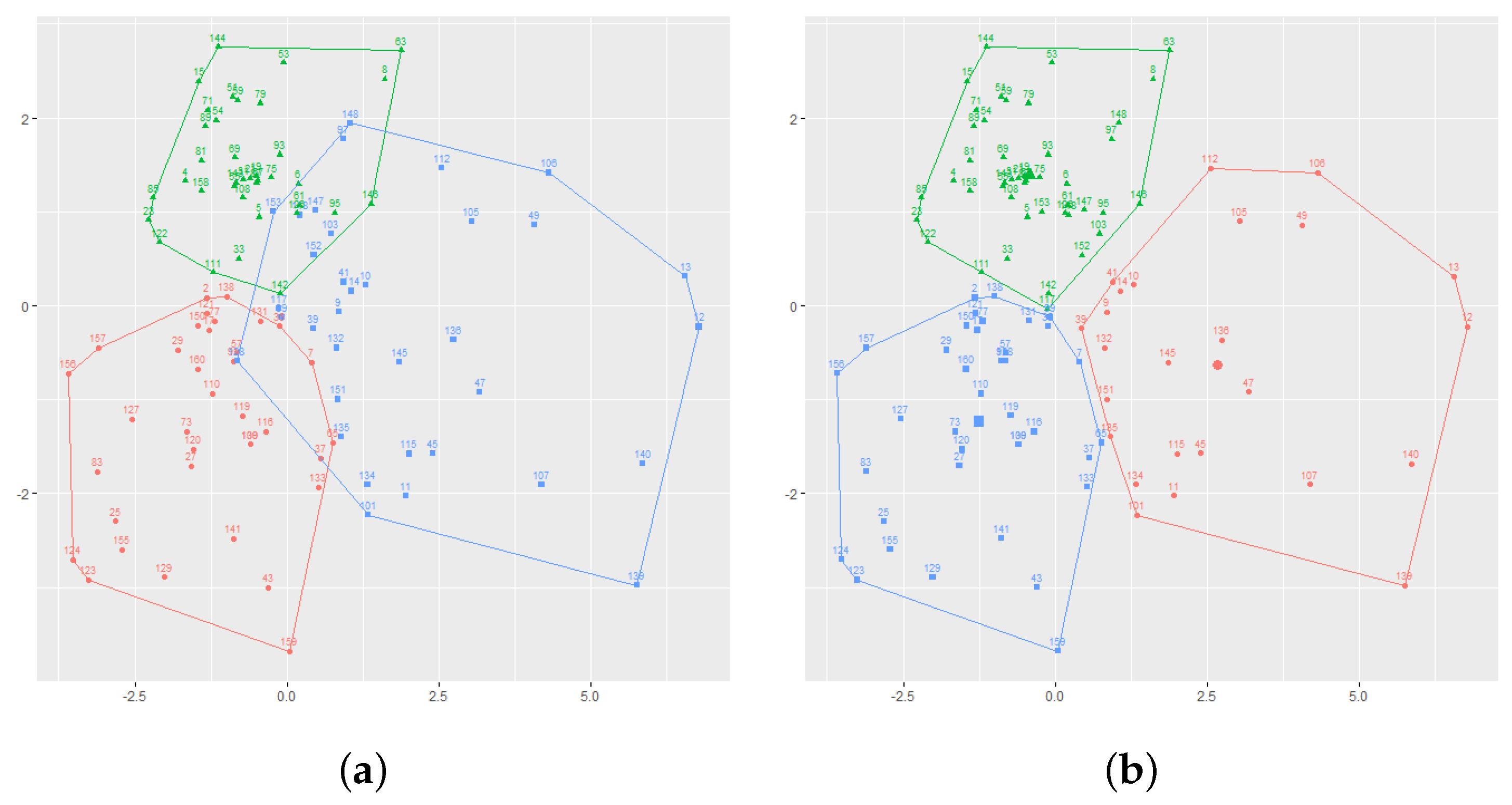
16), can be computed between the resulting partitions with the same number of clusters. Hence, for Kalundborg, the dissention degree between KD and FM was 0.11, which is a low dissention degree.
Figure 1 presents both partitions with respect to their first two principal components (the first and second components appear along the horizontal and vertical axes, respectively). On the other hand, for Bjerringbro, the dissention degree between KD and FM was of 0.006, which is an even lower dissention degree. That is, both partitions are almost identical.
Figure 2 presents both partitions. This measure on dissention provides some insight into the stability of the solution, as low values between the different possible solutions point out their consensus towards arriving at an optimal partition.
After learning the zones, we explore in the next section the potential of the proposed partitions for expected savings on the use of fertiliser.
4. Discussion
Following the results of the clustering methodology on the fields in Kalundborg and Bjerringbro, we can evaluate the impact of the management zones for decision-making on the application of fertiliser and their potential expected savings. Therefore, we compared the amount of fertiliser that would be applied on the field under a uniform dosage according to the Danish norm and under a site-specific treatment according to the requirements of each zone. In order to estimate the amounts of fertiliser that should be given to each zone, we took the mean amount of fertiliser that the parcels belonging to the same zone received under the initial experiments. In this way, we explored the potential savings that the management zones can have over the amounts of dosage on the field.
As mentioned above in
Section 2.2, the uniform dosage according to the Danish norm for winter wheat at Kalundborg is
kg/ha, while for Bjerringbro, it is
kg/ha. Then, by assessing the site-specific setting for the management zones obtained in
Section 3.2, the mean expected savings (by Equation (
2)) at Kalundborg added up to 52 kg/ha, which corresponds to the total mean savings (illustrated under Zone 0). On the other hand, for the crops at Bjerringbro, the expected mean savings added up to 52 kg/ha (again corresponding to the total mean savings illustrated under Zone 0). It should be stressed that such savings refer to the amount of fertiliser that would be applied according to the Danish norm, against the mean amount of fertiliser used in the site experiments. Hence, we did not control for the effects of applying different amounts of fertiliser on the yield or protein levels, although from a statistical point of view and as follows from the analysis of the experimental sites (see again
Section 3.1), the yield did not show significant differences with respect to the different fertilisation levels of 150, 200, and 300 kg/ha. In this sense, it can be expected that by reducing the amount of fertiliser inside those bounds of [150, 300], the yield would remain statistically similar to a uniform application of the Danish norm.
The complete results are shown in
Table 7 for Kalundborg and in
Table 8 for Bjerringbro, presenting the savings or losses for each zone and the amount of fertiliser (kg/ha) that would be applied under the proposed parcelwise configuration (recall that, for each zone, we took the mean dosage among all its member parcels). The number of parcels belonging to each zone is given under the column
Parcels, and Zone 0 illustrates the total mean results obtained under a uniform treatment where every parcel receives the same amount of 172 kg/ha at Kalundborg and 160 kg/ha at Bjerringbro, given by the total mean dosage of the initial experiments.
We can also examine in more detail the composition of each zone regarding its performance and potential for optimising the yield and quality of the harvest. In
Table 7 and
Table 8. we can see the mean levels for each zone, regarding the yield and protein contents. Taking into account the initial experimental measurements of
Table 2, it can be seen that the proposed management zones reconfigured the parcels aiming at optimising their mean performance on yield and quality.
Hence, for Kalundborg, three zones were identified with mean yield levels of 78.6, 81.9, and 89.8 hkg/ha. The higher amounts of yield correspond to a higher dose of 178 and 230 kg/ha, achieving also higher mean levels of protein content. For the third zone with the least fertiliser application, it should be noted that it accomplished higher levels than the ones obtained under the experimental dose of 50 kg/ha, while using less than the experimental optimum of 150 kg/ha.
Regarding the Bjerringbro site, nine zones were identified with mean yield levels ranging from 54.2 to 90.3 hkg/ha. In this case, the higher amounts of yield and quality do not necessarily correspond to higher levels of fertilisation, as, e.g., with 240 kg/ha, it obtained a mean yield of 90.3 hkg/ha; with 230 kg/ha, it achieved 84 hkg/ha; for a 166 kg/ha dose, it obtained a mean yield of 86.2 hkg/ha, but anyway achieving similar levels to the ones obtained in the experimental setting for a dose of 150 kg/ha and higher. On the other hand, focusing on the three zones with a mean dose of 50 kg/ha, the mean levels of yield and protein were approximately similar to the ones obtained under the initial experimental setting for the same amount of fertilisation, but Zone 1 suggests that some of the parcels that were given a 50 kg/ha application showed potential for achieving a greater level of yield and quality.
Overall, previously, it was identified that, under the initial experimental setting, the dose of 150 kg/ha achieved significantly equivalent results as the ones obtained with a greater dosage. With simulations and backward induction analysis inspired by the same field experiments in Denmark, it was found that variable rate nitrogen application could gain a potential differential gross margin between EUR 19 and 56 per ha based on a combination of sensor and soil information compared to uniform application [
21]. The proposed zones allow distinguishing which zones could be specifically treated to aim at higher yield and quality levels and which ones should be left for low yield and quality production. Then, a future study can be projected taking into account these management zones in the initial experiments, under the different fertilisation strategies, thus including from the beginning the soil and vegetation characteristics that local sensors allow capturing.
In [
22], it was concluded that the larger the difference in potential yield between zones, the more economic benefit from zone management. We used intra-field behaviour to describe differences within the field, and this difference is most probably also related to the difference in potential yield. However, a strategy based on past yield maps to develop management zones is not a good guide, and additional information is needed to predict nitrogen optima [
23]. We provided additional information that can be used to develop management zones. Another possibility is to use satellite data (see, e.g., [
24]), as models that rely solely on remote sensing data are comparatively less expensive than hybrid models.
5. Conclusions
An automatic methodology was proposed and validated for learning management zones, making use of local sensor data (vegetation and soil readings). Such a methodology optimises information measures regarding the relevance of the knowledge that is gathered by the specific zones (GAP), the explained variability (CH), the separation or how well identified the borders can be between groups (SIL), and the similarity between the parcels being grouped together (C-index).
As a result, fuzzy K-means (FM) and K-medoids (KD) achieved stable solutions according to the proposed dissimilarity degree (the partitions obtained under both methods were significantly similar). The impact of the algorithms was estimated for decision-making, and it remains for future research to harness the methodology so it optimises over a metric that adequately represents the preferences of the producers.
Regarding the explainability of the algorithm’s outcome, the expected savings were estimated based on the new management zones. For this case study, the expected savings were shown to be positive (following a uniform dosage strategy), having in mind that the mean productivity accomplished under the Danish norm can be even higher than the one accomplished under the experimental setting and that the amount of fertiliser that is actually used by farmers may vary from the norm for diverse uncontrollable reasons.
Besides, the case study presented in this paper suggests that the fertilisation strategies are not the only factor to take into account when trying to explain the different performances of the experimental parcels. In this sense, the inherent characteristics of the soil and vegetation are important factors to take into account. We are also aware that many other topics such as irrigation, nutrient form, and application method, together with the utilisation of the applied nutrient are related to the optimum fertilisation strategy, but this is out of the scope of the current study to explore.
This methodology sets a solid foundation based on vegetation and soil sensing, but it should be extended to consider topography and year-to-year variability, e.g., by the use of open data sources and specific on-site experiments collecting more historical observations on the behaviour of crops (while controlling all the relevant factors), including locally observed historical yield and quality data. Besides, other sources of information, such as market prices (affecting the desired level of quality to be achieved), should offer relevant knowledge for a more efficient and sustainable use of resources.
In a related line of research, it would be useful to build a model for predicting the optimal amount and timing of fertilisation that each zone requires according to its inherent (soil and vegetation) attributes and the desired levels of yield and quality. Such a model would involve understanding the behaviour of the crop under different conditions (such as the weather or topography), and it would allow obtaining much more precise estimates on the potential savings of the proposed methodology.


