Systemic Risk Contagion in China’s Financial–Real Estate Network: Modeling and Forecasting via Fractional-Order PDEs

Abstract

Modeling risk evolution in financial networks presents both practical and theoretical challenges, particularly during periods of heightened systemic stress. This issue has gained urgency recently in China as it faces unprecedented financial strain, largely driven by structural shifts in the real estate sector and broader economic vulnerabilities. In this study, we combine Fractional-order Partial Differential Equations (FoPDEs) with network-based analysis methods, proposing a hybrid framework for capturing and modeling systemic financial risk, which is quantified using the $\Delta CoVaR$ algorithm. The FoPDEs model is formulated based on reaction–diffusion equations and discretized using the Caputo fractional derivative. Parameter estimation is conducted through a composite optimization strategy, and numerical simulations are carried out to investigate the underlying mechanisms and dynamic behavior encoded in the equations. For empirical evaluation, we utilize data from China’s financial and real estate sectors. The results demonstrate that our model achieves a Mean Relative Accuracy (MRA) of 95.5% for daily-frequency data, outperforming LSTM and XGBoost under the same conditions. For weekly-frequency data, the model attains an MRA of 91.7%, exceeding XGBoost’s performance of 90.25%. Further analysis of parameter dynamics and event studies reveals that the fractional-order parameter $\alpha$, which controls the memory effect of the model, tends to remain low when $\Delta CoVaR$ exhibits sudden surges. This suggests that the model assigns greater importance to past data during periods of financial shocks, capturing the persistence of risk dynamics more effectively.

1. Introduction

The 2008 subprime mortgage crisis, though gradually fading from public memory, stands as a stark reminder of systemic financial risk. Its lessons are particularly relevant today, as concerns rise over a structural turning point in China’s real estate market since 2021 and the persistent, unrelenting decline in investment. While the 2008 crisis revealed the institutional and behavioral weaknesses that fuel systemic collapse, it left unresolved a critical question: how does systemic risk evolve in financial networks, and how can its emergence be detected and prevented?

Modeling risk evolution within financial networks presents practical challenges as financial systems are often highly interconnected, characterised by non-linear interactions and dynamic feedback loops [1]. Meanwhile, temporal dynamics further complicate the situation, as inter-connections and systemic behaviors evolve over time [2,3]. Computational complexity presents another obstacle, given that the large scale of financial networks requires efficient algorithms for simulation and analysis [4]. Furthermore, data quality and availability are often limited, constraining the reliability of network representations. Finally, bridging the gap between micro-level institutional behaviors and macro-level systemic dynamics also remains challenging [5]. Furthermore, in today’s financial environment, information propagates rapidly and economic conditions shift with increasing volatility. Therefore, it demands that models can simultaneously capture the non-linearity, temporal evolution, and causal dynamics of financial systems while maintaining the transparency of the structure for decision makers.

Various approaches have been developed to address the limitations of classical models. Non-linear regression methods, such as Generalised Autoregressive Conditional Heteroskedasticity (GARCH) models, extend linear models and offer improved capabilities for detecting complex patterns [6], while their variants have demonstrated effectiveness in capturing long-memory characteristics [7]. Machine learning techniques, by processing large-scale datasets through multi-layered structures, show promise in detecting subtle behavioral shifts. Recent efforts have also been made to address the black-box issue traditionally associated with machine learning, improving the interpretability of model parameters [8].

Despite the progress in financial risk modeling, significant challenges remain in accurately capturing long-range temporal dependencies, non-linear diffusion dynamics, and maintaining interpretability in complex financial systems. Traditional integer-order differential equations, though mathematically elegant, are fundamentally limited when modeling financial phenomena characterized by memory effects and persistent dependencies. Financial crises provide clear evidence of such persistent memory: the impact of past shocks continues to influence current risk dynamics far beyond what exponential decay models can capture [9]. Empirical studies further reveal power-law behaviors in financial time series, such as volatility clustering, heavy tails, and long-memory volatility processes [10].

To address these empirical regularities, fractional calculus offers a natural and powerful mathematical framework. The Caputo fractional derivative ${}^{C}D_t^{\alpha }$ of order $\alpha \in (0,1)$ incorporates a convolution kernel that weights all historical information according to a power-law decay, rather than the exponential decay implicit in classical models. This enables the model to capture non-Markovian dynamics, persistent shocks, and heterogeneous agent memory, and to bridge micro-macro dynamics in financial systems. Unlike integer-order models, where future states depend only on current conditions, fractional-order systems exhibit path dependence: the entire window history influences current evolution. This is particularly relevant for financial stress, which tends to propagate and persist over extended periods, creating “long tails” in crisis effects that fractional derivatives naturally represent. The fractional order $\alpha$ serves as a mesoscopic parameter, linking individual agent behaviors that are captured in network structures to system-level risk evolution modeled by the PDE.

Empirical evidence supports the use of fractional dynamics in finance: studies have documented fractional integration in volatility processes [9], long-memory in systemic risk measures [11], and power-law scaling in financial network properties [12]. For example, during the 2008 crisis, risk measures exhibited precisely the type of slow, persistent decay that fractional derivatives are designed to capture. Beyond empirical motivation, fractional PDEs offer superior modeling flexibility compared to the integer-order counterparts. The fractional order $\alpha$ provides an additional degree of freedom that can be calibrated to match empirical memory characteristics.

Recent advances have also demonstrated the effectiveness of fractional-order PDEs and network-based approaches in modeling diffusion processes across various domains, including biology and epidemiology [13,14]. These studies highlight the versatility of fractional calculus in capturing complex processes with memory effects and non-local interactions. Advances in computational methods have further revitalized PDE-based modeling by enabling the integration of fractional-order formulations that can capture the complex temporal dependencies characteristic of both biological and financial systems.

Further, compartment models using coupled Fractional Ordinary Differential Equations (FODEs) also provide robust theoretical foundations for financial contagion analysis [15] and show their flexibility in modeling complex networks. However, our study requires simultaneous modeling of temporal memory effects and spatial heterogeneity patterns across network nodes. The fractional reaction–diffusion PDE framework addresses this need by integrating time-dimensional memory with space-dimensional diffusion within a unified mathematical system, enabling comprehensive analysis of both risk generation and spatial propagation mechanisms.

Motivated by these considerations, this paper proposes a Fractional-order Partial Differential Equations (FoPDEs) framework to model the evolution of systemic risk in China’s financial–real estate networks. For empirical testing, we focus on systemic risk within the system, aiming to model and predict both the generation and contagion of risk across the system. The constructed network captures both direct and indirect connections between institutions, thereby preserving the true dynamics of risk evolution in real-world settings as much as possible. Specifically, we establish the network using both the Granger causality test and the Dynamic Correlation Coefficient (DCC) method, and measure systemic risk using the Delta Conditional Value-at-Risk ($\Delta CoVaR$) algorithm, estimated through the DCC-GARCH model.

The remainder of this paper is organized as follows: Section 2 describes the methodologies employed, including network theories, risk measurement techniques, and the FoPDEs framework. Section 3 introduces the dataset and data processing procedures. Section 4 presents the model fitting to actual financial data at both daily and weekly frequencies, followed by analyses based on the model results. Finally, Section 5 summarizes the main findings and contributions of the study.

2. Methodology

In this article, we investigate the generation and contagion of systemic risk mainly using three methodologies: network analysis, $\Delta CoVaR$- risk estimation, and the FoPDEs model and algorithms.

Using network and risk estimation methods, we capture the dynamics in the financial system and quantify the risk. Measures of network centrality, including degree, betweenness, and eigenvector centrality, play a fundamental role in identifying systemically important nodes within financial networks [16,17,18]. In recent studies, researchers found that the higher-order networks work well in describing the node interactions, especially in contexts where group behavior, coordination failure, or joint exposures dominate [19]. Granger causality models enable the exploration of directed temporal dependencies between institutions [20]. And to study systemic risk within financial networks, researchers also integrate network methods with risk measures [21,22].

For modeling and forecasting the risk evolution in the system, we turn to contagion models. FoPDEs have shown their superiority in capturing non-linearity and dynamics in the biology field, especially in modeling non-local interactions and memory effects in complex systems, offering good perspectives on the temporal and spatial evolution of systemic risk [23,24,25,26]. Dynamic network models account for temporal variations in financial linkages, thus capturing the evolving structure of interconnections [2,27]. Furthermore, DebtRank [28,29] and epidemic models, such as SIS and SIR [30,31,32], simulate the spread of distress across networks, allowing for the quantification of potential failures. And Agent-Based Models (ABMs) simulate the behavior of individual institutions under stress to uncover emergent systemic patterns [33,34].

2.1. Network Methods

Network theory offers a powerful framework for analyzing complex systems characterized by connectivity, interactions, and dynamics [35,36]. This approach is particularly suited to capture both direct and indirect dependencies among financial networks [37]. In addition, networks also serve as a foundation for other analytical methods to study system resilience and risk management strategies. Techniques like higher-order motifs and clustering are deployed to delve deeper into the structure of the system [38,39].

2.1.1. Edge Determination in Network

To determine the directions of edges in the network, we employ the Granger causality framework [40,41]. For each pair of nodes, once the return series are confirmed to be stationary, we apply the Granger causality test (implemented in Python using statsmodels.tsa.stattools.) to assess directional dependence. Details of the test procedure are provided in Appendix A. We retain both directions between any pair of nodes if they each pass the causality test to better preserve and reflect the structure of the system.

Moreover, the test also serves as an adaptive thresholding mechanism to filter out spurious connections and reduce network complexity, making the network sparser. This data-driven approach offers advantages over fixed-value methods, as the former gives each pair a specific threshold, better reflecting the dynamic interdependencies among different financial institutions [42,43].

Upon the presence of edges with directions between the nodes, DCC is then used to decide on the edge weights [44]. DCC is an extension of the GARCH model that allows for time-varying correlations between multiple time series. In the context of financial networks, DCC captures how the correlations between institutions’ returns evolve over time. Thus, a higher ${\rho }_{i,j}^t$ implies a stronger dynamic correlation between institutions i and j, indicating a more significant connection in the network.

Let $G=(V,E)$ denote the financial network, where V is the set of nodes representing financial institutions and E is the set of edges. For each $e_{i,j}\in E$, the weight $w_{i,j}$ is assigned as the time-averaged ${\overline{\rho }}_{i,j}$, provided that the node pair $v_{i,j}$ passes the Granger causality test. The combination of the causality test and the DCC model contributes to building a sparse and informative network that can capture the risk of contagion between nodes.

$$w_{i,j}=\left\{\begin{array}{cc}{\overline{\rho }}_{i,j}& Grange{r}_{i,j}=True\\ 0& Grange{r}_{i,j}=False\end{array}\right.$$

(1)

2.1.2. Motif Filtering and Clustering

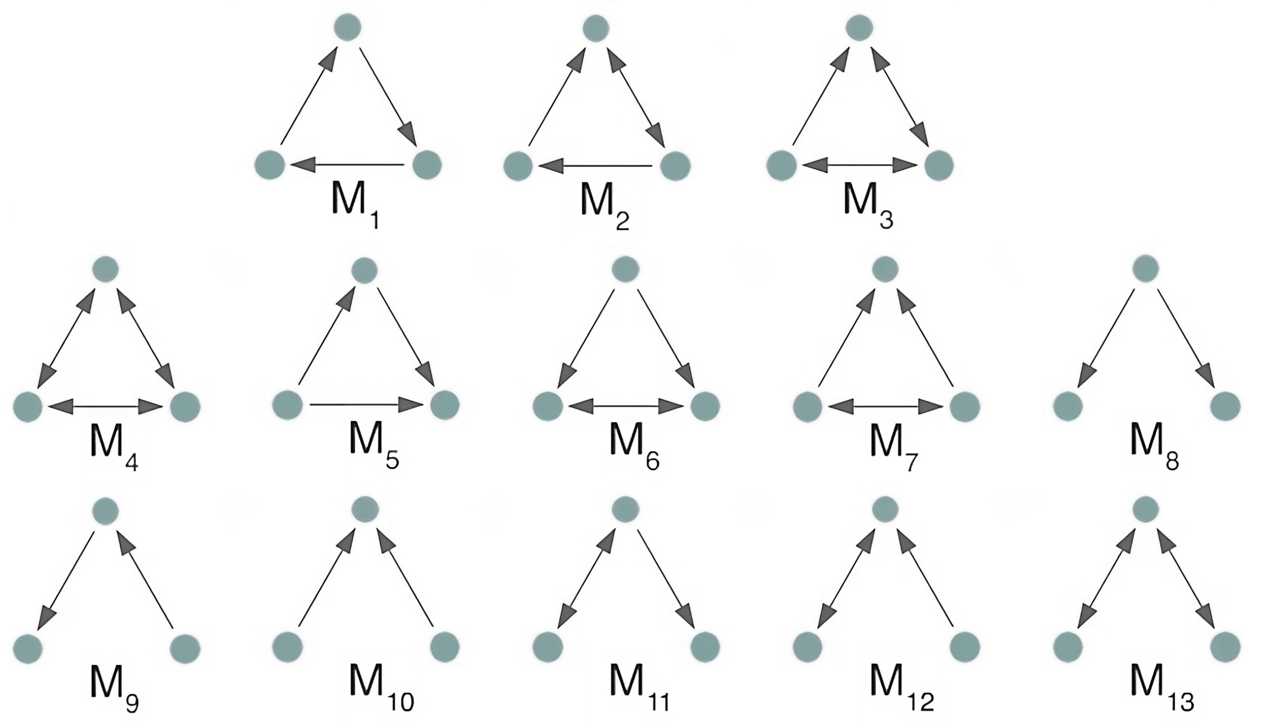
The basic network is constructed by capturing all statistically significant causal relationships. However, to focus on the evolution mechanisms, we seek to identify and retain only structural patterns that represent the contagion processes, while filtering out less relevant connections. A robust approach is to apply motif-based clustering techniques. Motifs, initially proposed for the study of complex biological networks [39,45], serve as fundamental tools in directed networks. On one hand, this framework enables the identification of higher-order structures by focusing on one or multiple motifs of interest. On the other hand, it facilitates the evaluation of which motifs are statistically significant within a network and are thus most informative for understanding its underlying dynamics [38]. Dozens of patterns of motifs have been defined, and the details are shown below in Figure 1.

To capture the key characteristics of risk diffusion within the financial system, we adopt the Motif-8 structure (see Figure 2). Motif-8 highlights the structural feature whereby a node can transmit influence to multiple downstream nodes, reflecting typical dynamics of risk diffusion. This pattern is analogous to the evolution of viruses or chemical substances, which move from areas of higher concentration to areas of lower concentration.

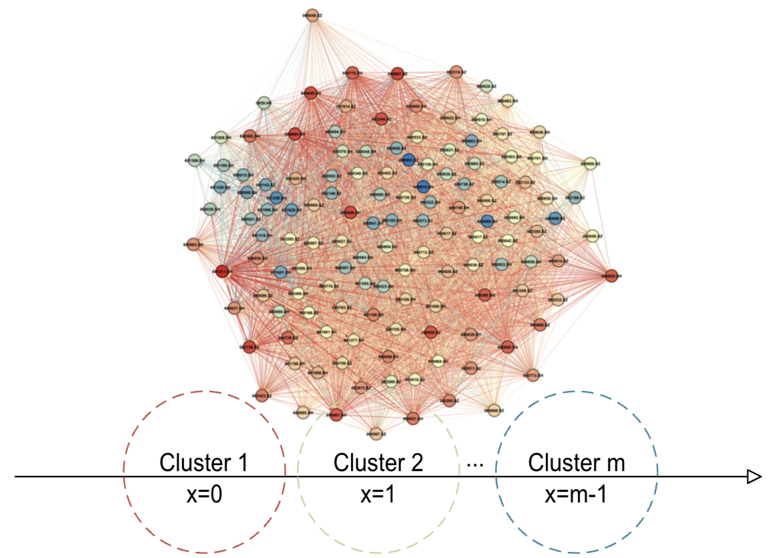
Clustering gathers together groups of nodes with stronger internal relationships, thereby identifying the pathways through which risk propagates both within and across clusters (see Figure 3). In this work, we apply the K-means algorithm (see Algorithm A1 in Appendix C) for clustering [46,47]. We determine the number of clusters by combining the Elbow method and domain knowledge, in line with our objective of modeling risk diffusion from high-risk, through moderate-risk, to low-risk segments. Within each cluster, stronger correlations among nodes facilitate more rapid risk diffusion, whereas inter-cluster transmission is comparatively restricted. It is worth noting that clustering results may evolve over time, reflecting the dynamic nature of inter-institutional relationships.

It is worth noting that the choice of m (the number of clusters) primarily reflects the economic structure and risk segmentation within the financial network and is determined by empirical analysis and interpretability. In the subsequent numerical procedures, the spatial domain $[0,m-1]$ is further discretized into M grid points for FoPDE computation, where M can be any integer greater than m to ensure sufficient numerical accuracy. The discretization process is general and remains valid for any $m>2$; the specific value of m does not affect the applicability of the numerical scheme, but rather influences the granularity of risk segmentation and the economic interpretation of the clusters. Therefore, while m is chosen for interpretability and empirical relevance, the numerical solution of the FoPDE is robust to this choice as long as $m>2$.

In this study, we make a methodologically sound simplification by assuming a fixed network structure once it has been reliably established. This assumption is justified by the following considerations. First, empirical evidence suggests that the structure of financial networks exhibits relative stability over short- to medium-term horizons [37]. In the financial context, this stability can be attributed to regulatory oversight of listed entities and the relatively stable business relationships constrained by contracts and legal frameworks. Second, the DCC parameter ${\rho }_{i,j}^t$ contributes to capturing temporal dynamics within this established structure. These dynamic correlations represent the evolving strength of relationships between institutions, allowing the model to adapt to changing market conditions, stress periods, and policy interventions without requiring alterations to the underlying network structure.

Future research could address these limitations through regime-switching models that allow topology changes at structural break points or adaptive network learning algorithms that update connectivity based on rolling correlation windows. But such structures could require re-estimating network topology at each time step, leading to a dramatic surge in computational complexity.

2.2. Measurement of the Systemic Risk

In finance, systemic risk refers to the potential for a collapse of an entire financial system. Various methods have been developed to measure systemic risk, each addressing different aspects of this complex phenomenon. One widely used approach is Conditional Value at Risk ($CoVaR$), introduced by [48], which quantifies the risk of a financial system conditional on an institution being in distress. Another method is Systemic Expected Shortfall (SES), proposed by [49], which measures the contribution of a financial institution to systemic risk by assessing its expected losses during a crisis. Furthermore, Marginal Expected Shortfall (MES), developed by [50], captures an institution’s vulnerability to systemic risk by analyzing its losses during extreme market conditions.

To capture time-varying interdependencies and comovements in tail risk, we combine Adrian and Brunnermeier’s CoVaR framework [51] with a Dynamic Conditional Correlation GARCH (DCC-GARCH) model [52,53] to estimate institution-specific systemic risk contributions [54]. This integration brings several advantages. First, the DCC structure models time-varying risk contagion through dynamic correlations, denoted by ${\rho }_{i,s}^t$, which reflects evolving financial linkages between institution i and the system s. Second, the use of univariate GARCH(1,1) modeling for the system return series captures conditional heteroskedasticity, enabling volatility scaling via ${\sigma }_s^t$ and thus enhancing the robustness of risk estimates under different market regimes. Third, the multivariate GARCH framework preserves non-linear dependencies and tail comovements, which are critical for systemic risk measurement. More advanced structures like DCC-EGARCH have been proposed recently to incorporate asymmetric volatility effects through an additional parameter $\gamma$ [55], which further improves the robustness of the model.

However, for computational efficiency and compatibility, we adopt the DCC-GARCH(1,1) model implemented via the Python package frds.algorithms (https://frds.io/algorithms/garch/, accessed on 8 July 2025). For each institution–system pair, the dynamic correlation ${\rho }_{i,s}^t$ is estimated using DCC-GARCH, while the system’s conditional volatility ${\sigma }_s^t$ is obtained from a separate univariate GARCH(1,1) model. To validate model adequacy, an ARCH–LM test is conducted on the residuals ${ϵ}_s^t$ to confirm the absence of remaining ARCH effects. The $\Delta \mathrm{CoVaR}$ of institution i with respect to the system s is computed as:

$$\Delta CoVa{R}_{s|i}^{t,q}={\Phi }^{-1}\left(q\right){\rho }_{i,s}^t{\sigma }_s^t,$$

(2)

where ${\Phi }^{-1}\left(q\right)$ is the quantile function of the standard normal distribution. Detailed implementation is provided in Appendix B.

Network-Weighted Risk Aggregation

Existing approaches to estimating cluster-level systemic risk often rely on averages, which can lead to a loss of tail information and obscure the heterogeneity among institutions [56]. To address these shortcomings, two improved methodologies are considered: the index-based approach and the network-edge weighting method. The index-based method constructs a portfolio for each cluster by calculating the $\Delta \mathrm{CoVaR}$ between this synthetic index and the system. However, it implicitly assumes linear risk scaling with institutional size, an assumption that may not align with empirical observations during crises [57]. By contrast, the network-edge weighting method explicitly models two contagion mechanisms. First, direct exposure channels are captured through direct connecting edges, reflecting default cascades. Second, indirect connectivity effects are incorporated by broader network topology, whereby highly connected nodes amplify shocks through higher-order structures. Moreover, the network-edge approach offers additional advantages as it captures non-linear risk diffusion and can identify small but critically interconnected entities that size-based methods might overlook. Given these strengths, we adopt the network-edge weighting method to assess the total risk contribution of clusters of nodes to the system.

For Cluster c with a set of nodes $V_c$, cluster-level $\Delta CoVaR$ values are weighted by their edge weights to the whole network edges [58]:

$$\Delta CoVa{R}_c^q=\sum _{i\in V_c}{\displaystyle \frac{{\sum }_{j\in V_c}{w}_{i,j}}{{\sum }_j{\sum }_{k\in V_c}{w}_{k,j}}}·\Delta CoVa{R}_i^q$$

(3)

where $w_{ij}$ denotes the weights between institutions i and j, as defined in Equation (1).

This approach explicitly links systemic risk contributions to an institution’s topological significance within the network, as captured by the weights of its incident edges. By incorporating higher-order Motif-8 structural filtering, we anticipate that the resulting clusters will exhibit distinct average levels of $\Delta CoVaR$, indicative of heterogeneous systemic risk exposure (see Figure 4).

By employing network and clustering methods, we project the risk distribution across the financial network onto a one-dimensional space, which constitutes the spatial dimension in our FoPDEs model. Specifically, clusters are sorted in descending order based on $\Delta CoVaR$. This ordering is motivated by the empirical observation that risk tends to originate from highly interconnected and volatile segments and subsequently propagates towards more stable entities. While this approach abstracts from the full complexity of network topology, it provides a meaningful spatial representation of risk flow: high-risk clusters function as sources of contagion, while lower-risk clusters serve as absorbers. Moreover, since intra-cluster linkages are typically denser than inter-cluster ones, this ordering helps capture the directional nature of diffusion. Thus, although simplifications are inherent, this cluster-based spatial mapping aligns well with the qualitative dynamics of risk propagation and is validated by the effectiveness of the FoPDEs model in empirical forecasting tasks [59].

Following our previous methodology [22], this spatial embedding employs a dual-criterion approach to ensure both economic relevance and structural consistency. First, clusters are primarily ordered by their mean $\Delta CoVaR$ values, reflecting overall systemic risk concentration levels and capturing the empirical regularity that financial stress typically originates in high-risk segments and propagates toward more stable institutions [60]. Second, the spatial proximity among different clusters can be measured by the degree of their inter-ethnic connections, reflecting the principle where risk transmission affects closely connected institutions first before spreading to more distant entities [61]. We define the distance between two clusters by using the sum of edge weights of connecting these clusters. The spatial ordering will be determined at the beginning of the analysis period and remains fixed throughout the study. The resulting spatial coordinate $x\in [0,m-1]$ thus represents positions along a systemic risk spectrum, providing a mathematically tractable framework for modeling risk-gradient diffusion dynamics while preserving the essential economic interpretation of contagion patterns.

2.3. Fractional-Order PDEs

Building upon previous research [22] and the framework outlined in [62], we propose a fractional-order reaction–diffusion equation for modeling risk dynamics within financial networks. By integrating fractional calculus with non-linear reaction terms, the model captures key empirical features of financial crises, particularly the long-term dependence observed in systemic risk evolution. Compared with classical PDE-based models and data-driven machine learning approaches, our formulation combines the advantages of historical memory effects and parameter interpretability, while simultaneously achieving a satisfying level of forecasting accuracy.

The incorporation of fractional derivatives in our model is motivated by both macroeconomic theory and empirical evidence from our analysis. From a macroeconomic perspective, systemic risk measures exhibit well-documented dependence on historical data and long-range temporal memory [63,64], with the mathematical structure of the fractional time derivative directly corresponding to the historical dependence and long-range memory resulting from power-law waiting times in financial systems. Our parameter analysis (Section 2.3.4) demonstrates statistically significant relationships between the fractional order $\alpha$ and risk dynamics, where $\alpha$ tends to decrease during periods of elevated systemic risk, indicating the model’s adaptive mechanism to automatically adjust memory effects during financial stress periods. In the financial context, fractional derivatives capture information processing delays among market participants, institutional memory in risk assessment, and regulatory response lags, with the fractional order $\alpha$ providing a mesoscopic bridge between individual institution behaviors and system-level risk evolution.

2.3.1. Model Formulation

For a total of m clusters, we employ a continuous spatial embedding approach where the discrete cluster indices are mapped to a continuous spatial domain. Let $u(x,t)\in [0,K]$ represent the systemic risk level, denoted as $\Delta CoVa{R}_c^q$ in Equation (3), at spatial position $x\in [0,m-1]$ and time $t\ge 0$, where the continuous spatial coordinate x represents the embedded positions of the discrete clusters ($x=0,1,\dots ,m-1$ correspond to Clusters 1, 2, …, m respectively). Here, K denotes the maximum capacity of systemic risk, and when risk concentration exceeds this threshold, systemic collapse may occur.

The continuous PDE formulation serves as a mathematical approximation to capture risk diffusion dynamics between clusters, where spatial derivatives represent the tendency for risk to flow from high-concentration clusters to neighboring clusters through network interconnections. Economically, this “diffusion” represents various channels of risk transmission: direct exposures through counterparty relationships, indirect contagion through market liquidity effects, correlated asset price movements, and behavioral spillovers such as confidence crises or flight-to-quality dynamics. The spatial ordering of clusters (from high-risk to low-risk) captures the empirical observation that financial stress typically originates in the most vulnerable segments and propagates towards more stable institutions.

This approach is justified by the spatial discretization scheme (detailed in Section 2.3.2), which interpolates the discrete cluster values onto a continuous grid, enabling the application of numerical methods. The equations combine Caputo time-fractional derivative with spatially heterogeneous diffusion:

$$\left\{\begin{array}{c}{\displaystyle {}^{C}D_t^{\alpha }u={\partial }_x\left(D\left(x\right){\partial }_{x}u\right)+R\left(u\right)+b·\mathrm{sign}\left({\partial }_{x}u\right)}\hfill \\ u(x,0)=\phi \left(x\right),0<x<m-1\hfill \\ {\partial }_{x}u{{|}_{x=0}={\partial }_{x}u|}_{x=m-1}=0,t>0,\hfill \end{array}\right.$$

(4)

where ${}^{C}D_t^{\alpha }$ denotes the Caputo fractional derivative of order $\alpha \in (0,1)$, defined as [65]:

$${}^{C}D_t^{\alpha }u(x,t)={\displaystyle \frac{1}{\Gamma (1-\alpha )}}{\int }_0^t{(t-\tau )}^{-\alpha }{\partial }_{\tau }u(x,\tau )d\tau .$$

(5)

The Caputo fractional derivative encodes memory effects through the convolution kernel. And the right-hand side of the FoPDEs consists of diffusion term, non-linear interaction, and direction-sensitive forcing:

• ${\partial }_x\left(D\left(x\right){\partial }_{x}u\right)$ models risk transmission through transboundary connections, with $D\left(x\right)$ representing the spatially varying diffusion coefficient determined by cluster features. The function $D\left(x\right)$ is defined as a continuous function over the interval $[0,m-1]$, where it takes prescribed values $d_1,d_2,\dots ,d_m$ at the discrete points $x=0,1,\dots ,m-1$, respectively. These values $d_i$ represent the risk diffusion coefficients for each cluster i. And to ensure smoothness across cluster boundaries, we employ the not-a-knot cubic spline [66] interpolation method to construct $D\left(x\right)$. This interpolation approach, implemented through the scipy.interpolate package (default in scipy.interpolate.CubicSpline, https://docs.scipy.org/doc/scipy/reference/generated/scipy.interpolate.CubicSpline.html; accessed on 20 August 2025), guarantees that the resulting function $D\left(x\right)$ possesses continuous second derivatives throughout the entire interval $[0,m-1]$, thereby providing a smooth transition of diffusion properties between adjacent clusters while preserving the prescribed diffusion characteristics at each cluster location.
• $R\left(u\right)$ is the non-linear reaction term given by

  $$R=Au(h\left(x\right)-u/K)+B{e}^{-C{(u/K)}^2}u,$$

  (6)

  where,
  • $Au\left(h\right(x)-u/K)$ is the logistic regulation, reflecting capital adequacy requirements and preventing unbounded risk growth.
  • The function $h\left(x\right)$ governs the spatial variation of risk spreading across different regions or clusters, reflecting heterogeneity arising from structural differences within financial sub-networks. In our implementation, we simplify the model by setting $h\left(x\right)\equiv h$, as empirical results indicate that spatial variation in h has limited impact on the overall risk dynamics $u(x,t)$, while this simplification significantly reduces the computational complexity.
  • The Gaussian thresholding term, $B{e}^{-C{(u/K)}^2}$, introduces a non-linear damping effect. This mechanism becomes significant when $u/K>1/\sqrt{2C}$, corresponding to scenarios such as liquidity dry-ups or sudden market freezes.
• The directional term $b·\mathrm{sign}\left({\partial }_{x}u\right)$ is introduced as a behavioral and policy-driven drift component, representing the market response to perceived risk gradients. In times of high uncertainty, this drift captures how pessimistic sentiment, herd behavior, and anticipatory reactions accelerate the spread of risk towards relatively safer areas. Conversely, well-timed policy actions can guide this directional flow in a stabilizing manner, effectively reversing or slowing down the propagation of distress across the network.
• Initial function $u(x,0)=\phi \left(x\right)$ is set as $\Delta CoVa{R}_c^q$ calculated with Equation (3) at time $t=0$.
• Parameters $\theta =(\alpha ,A,B,C,h,b,K,d_1,d_2,d_3)$ are to be initialized and subsequently optimized using observed data. Optimization is conducted on a moving-window basis, enabling the model to adapt to evolving market conditions. For each time window, once these parameters are determined the FoPDEs model is established and employed to generate forecasts.

The risk-gradient diffusion term ${\partial }_x\left(D\left(x\right){\partial }_{x}u\right)$ captures financial contagion mechanisms following the empirical pattern where risk first affects entities with close connections, then subsequently affects entities with weaker connections, mirroring spatial diffusion processes across the systemic risk spectrum. This formulation operates under the assumption that direct connections between distant risk clusters (e.g., Clusters 1 and 3) are relatively weak compared to connections between adjacent risk levels, thereby justifying the local diffusion approximation that provides an appropriate mathematical structure for describing risk propagation processes. We acknowledge that this approach represents a simplification of the actual network structure, as direct connections do exist between non-adjacent clusters in reality. However, our empirical network analysis indicates that edge weights connecting distant clusters are relatively small compared to adjacent cluster connections, with the strongest transmission patterns occurring between clusters with similar risk profiles, thus validating our one-dimensional spatial projection based on weak long-range connectivity. However, if strong direct connections existed between all cluster pairs, a two-dimension space diffusion structure or coupled system approaches such as compartment models might be more appropriate for capturing the full complexity of inter-cluster interactions.

2.3.2. Numerical Discretization

To numerically solve Equation (4), we adopt an Implicit–Explicit (IMEX) time-stepping method [67] that integrates the memory effect of the Caputo fractional derivative with efficient spatial diffusion discretization. For each sliding window of length L, we interpolate the data onto a uniform space–time grid of size $M\times N$, where M and N denote the number of spatial and temporal nodes, respectively.

• Time Discretization
  The temporal domain is partitioned with a uniform time step $\Delta t$, such that $t_n=n\Delta t$, where $n=0,1,2,\dots ,N-1$ indexes the inner discrete time levels up to the final time $L=(N-1)\Delta t$. Following the scheme for the Caputo fractional derivative of order $\alpha \in (0,1)$ [62,65], we approximate at $t_n$:

  $${}^{C}D_t^{\alpha }{u}^n\approx {\displaystyle \frac{{(\Delta t)}^{-\alpha }}{\Gamma (2-\alpha )}}\sum _{k=0}^{n-1}{w}_k^{\left(n\right)}(u^{k+1}-u^k),$$

  (7)

  where the nonuniform memory weights $w_k^{\left(n\right)}$ are defined by:

  $$w_k^{\left(n\right)}={(n-k)}^{1-\alpha }-{(n-k-1)}^{1-\alpha }.$$
• Space Discretization
  The transition from discrete cluster indices to continuous spatial derivatives is handled through spatial discretization and interpolation. In the mathematical formulation, we map the cluster labels to spatial positions as Cluster 1 ↔$x=0$, Cluster 2 ↔$x=1$, and Cluster 3 ↔$x=2$. The spatial domain $[0,m-1]$ is then discretized into M uniformly spaced grid points with spatial step size $\Delta x={\displaystyle \frac{m-1}{M-1}}$. The grid points are indexed as $i=0,1,2,\dots ,M-1$, with corresponding spatial locations $x_i=i·\Delta x$, such that $x_0=0$ and $x_{M-1}=m-1$ correspond to the cluster boundaries.
  The discrete cluster risk values are interpolated onto this continuous grid using not-a-knot cubic-spline interpolation. Specifically, the diffusion coefficient $D\left(x\right)$ is computed as $D_i=D\left(x_{i-1}\right)$ with boundary values $d_1=D\left(x_0\right)$, $d_m=D\left(x_{M-1}\right)$, and intermediate values are obtained through smooth interpolation. This approach transforms the discrete cluster-based risk measures into a continuous field suitable for PDE analysis, while preserving the essential characteristics of inter-cluster risk transmission. The discretized diffusion operator is given by:

  $${\partial }_x\left(D\left(x\right){\partial }_{x}u\right){|}_i\approx {\displaystyle \frac{D_{i+1/2}(u_{i+1}-u_i)-D_{i-1/2}(u_i-u_{i-1})}{{(\Delta x)}^2}},$$

  (8)

  with interface diffusion coefficients defined by:

  $$D_{i\pm 1/2}={\displaystyle \frac{D_i+D_{i\pm 1}}{2}},$$

  and to maintain consistency with homogeneous Neumann boundary conditions ${\partial }_{x}u{{|}_{x=0}={\partial }_{x}u|}_{x=m-1}=0$, we employ ghost point extrapolation for $D_{-1}=D_0$ and $D_M=D_{M-1}$. To promote the calculation efficiency, we deploy symmetric tridiagonal diffusion matrix $D_{\mathrm{mat}}$ of order M [62] on vector $U={(u_0,u_1,\cdots ,u_{M-1})}^T$ to get spatial discretisation:

  $${\left(D_{\mathrm{mat}}U\right)}_i={\displaystyle \frac{1}{{(\Delta x)}^2}}\left[-D_{i-1/2}{u}_{i-1}+(D_{i-1/2}+D_{i+1/2})u_i-D_{i+1/2}{u}_{i+1}\right]$$

  with

  $$D_{\mathrm{mat}}={\displaystyle \frac{1}{{(\Delta x)}^2}}\left[\begin{array}{ccccc}-D_{{\displaystyle \frac{1}{2}}}& D_{{\displaystyle \frac{1}{2}}}& 0& \dots & 0\\ D_{{\displaystyle \frac{1}{2}}}& -(D_{{\displaystyle \frac{1}{2}}}+D_{{\displaystyle \frac{3}{2}}})& D_{{\displaystyle \frac{3}{2}}}& \dots & 0\\ 0& D_{{\displaystyle \frac{3}{2}}}& -(D_{{\displaystyle \frac{3}{2}}}+D_{{\displaystyle \frac{5}{2}}})& \ddots & ⋮\\ ⋮& \ddots & \ddots & \ddots & D_{M-{\displaystyle \frac{3}{2}}}\\ 0& \dots & 0& D_{M-{\displaystyle \frac{3}{2}}}& -D_{M-{\displaystyle \frac{3}{2}}}\end{array}\right].$$
• Unified IMEX Update Equation
  Let ${\gamma }_{\alpha }={(\Delta t)}^{\alpha }\Gamma (2-\alpha )$; the evolution of the system at each time step $n+1$ is governed by:

  $$\left(I-{\gamma }_{\alpha }{D}_{\mathrm{mat}}\right)·U^{n+1}=U^n+{\gamma }_{\alpha }R\left(U^n\right)+{\gamma }_{\alpha }b·\mathrm{sign}\left({\partial }_x{U}^n\right)-H^n,$$

  (9)

  where
  • I is an identity matrix of order M and $I-{\gamma }_{\alpha }{D}_{\mathrm{mat}}$ is an invertible symmetric tridiagonal matix;
  • $R\left(U^n\right)={(R_0^n,R_1^n,\cdots ,R_{M-1}^n)}^T$ is the reaction term;
  • $H^n$ is the history term with $H_i^n={\sum }_{k=1}^n{w}_k^{\left(n\right)}(u^k-u^{k-1})$ for $i=1,2,\dots ,M-1$;
  • $\mathrm{sign}\left({\partial }_x{U}^n\right)$ is the drift term with $\mathrm{sign}{\left({\partial }_x{u}^n\right)}_i\approx \mathrm{sign}\left({\displaystyle \frac{u_{i+1}^n-u_{i-1}^n}{2\Delta x}}\right)$ for $i=1,2,\dots ,M-1$.

2.3.3. Parameter Optimization

Due to the high dimensionality of the parameter space, we adopt a two-stage optimization strategy: an initial global search is conducted using the Dual Annealing (DA) algorithm (see Algorithm A2), followed by a local refinement using the Trust-Region Constrained (Trust-Constr, TC) method. The details of the parameter optimization are provided in Appendix D.

The model parameters $\theta =(\alpha ,A,B,C,h,b,K,d_1,...,d_m)$ are decided by solving the following constrained regularized minimization problem:

$$\begin{array}{cc}\hfill {\widehat{\theta }}_t=arg\underset{\theta }{min}& \left\{{\displaystyle \frac{1}{M·N}}\sum _{i=0}^{M-1}\sum _{k=0}^{N-1}{\left(u_{\mathrm{obs}}(x_i,t_k)-u_{\theta }(x_i,t_k)\right)}^2+\lambda {\parallel \theta \parallel }^2\right\}\hfill \\ \hfill \mathrm{subject}\mathrm{to}& \alpha \in (0.1,0.99),A,B,C\in (0.01,1.0),\hfill \\ \hfill & h\in (0.1,3.0),K\in (5.0,20.0),\hfill \\ \hfill & d_1,...,d_m\in (0.1,3.0),b\in (-5.0,5.0).\hfill \end{array}$$

(10)

Here, $u_{\mathrm{obs}}$ denotes the observed state of the system and $u_{\theta }$ is the numerical solution of the PDE system given parameter vector $\theta$. The second term imposes Tikhonov (ridge) regularization to mitigate overfitting. The explicit parameter bounds, in this paper, refined through extensive numerical simulations (see Section 2.3.4) and experimentation with the database to ensure optimal convergence, numerical stability and computation efficiency, are enforced throughout the optimization process.

This approach yields a robust estimate ${\widehat{\theta }}_t$ for each window, which is then used to generate predictions for the subsequent time horizon. Recalibration is triggered adaptively when the forecast error in the latest step exceeds a predefined tolerance ${ϵ}_{\mathrm{tol}}=2{\sigma }_{\mathrm{noise}}$, where ${\sigma }_{\mathrm{noise}}$ represents the empirical standard deviation of the measurement noise.

2.3.4. Numerical Simulation

Given the parameters and initial values, the subsequent states of the FoPDEs system can be computed using the numerical scheme. The numerical simulations show how parameter variations influence system dynamics, providing insights into potential directions for model optimization through parameter adjustment.

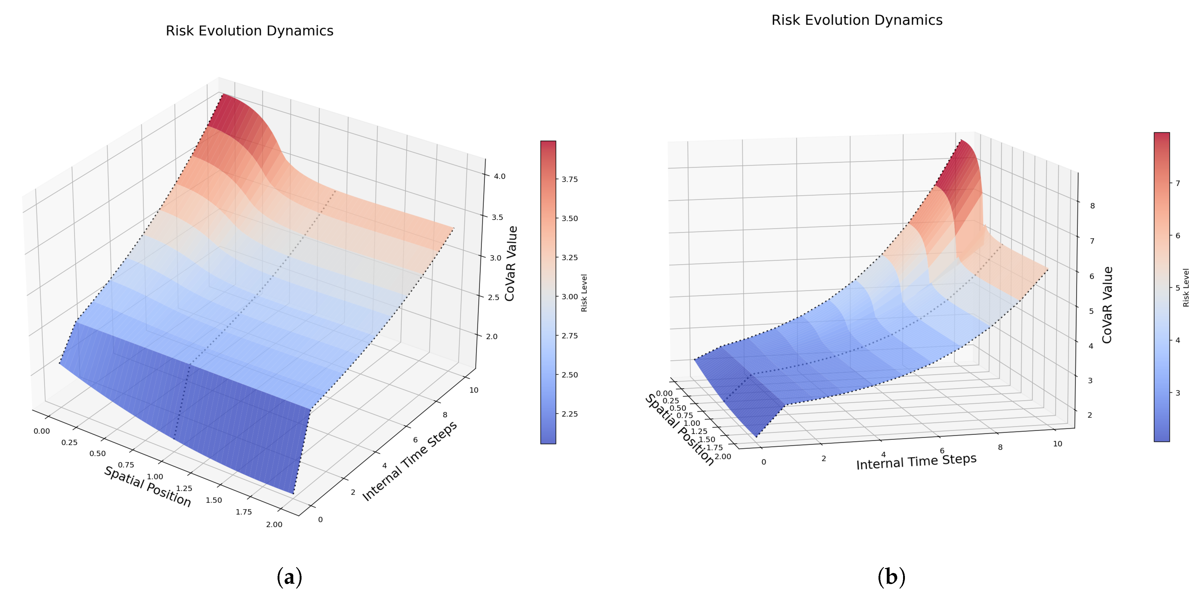
Here we initialize the simulations with data from our case where $m=3$, which means three clusters are formulated and the parameters to be optimized are fixed to $\theta =(\alpha ,A,B,C,h,b,K,d_1,d_2,d_3)$. Figure 5 presents an overview of the FoPDEs model dynamics and highlights the effects of altering the fractional-order parameter $\alpha$ from its optimized value. The results reveal substantial changes in the system’s evolution when $\alpha$ is varied. 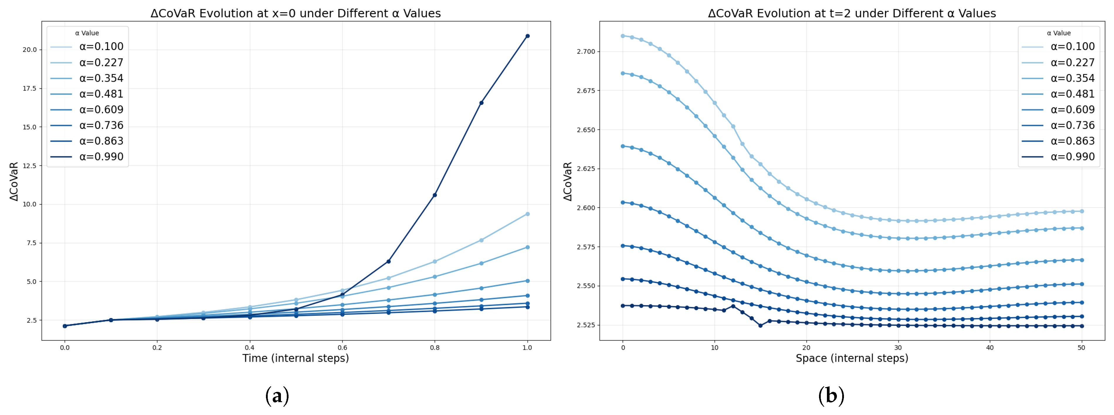Further analysis is presented in Figure 6, where several values of $\alpha$ are selected to plot the system’s dynamics along temporal and spatial dimensions at a single time or space step. The resulting curves vary significantly with $\alpha$, reflecting the distinct influence of memory effects. Specifically, in the time dimension the system exhibits smooth and continuous evolution, while in the spatial dimension additional fluctuations emerge—illustrating the heterogeneous nature of different positions, primarily influenced by the parameters $d_1$, $d_2$, and $d_3$.

Figure 7, Figure 8 and Figure 9 explore the impact of other key parameters on the system’s dynamics. In Figure 7, the diffusion-related parameters $d_1$, $d_2$, and $d_3$ exhibit similar effects across spatial positions, resulting in analogous curve patterns. Figure 8 and Figure 9 further illustrate how variations in parameters A, B, C, h, b, and K modulate the behavior of the FoPDEs model.

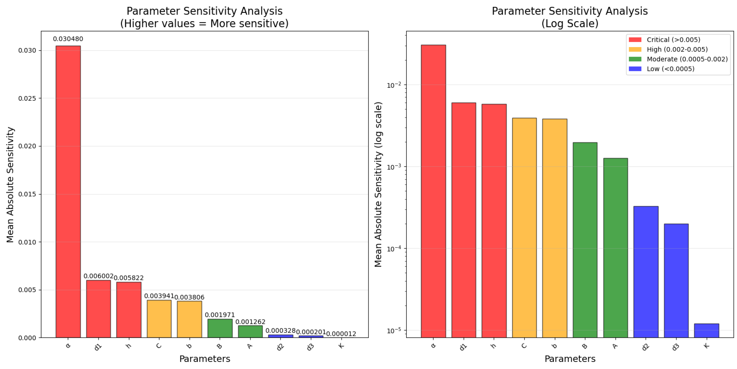
To systematically evaluate parameter importance in our fractional-order PDE risk model, we conducted a finite difference sensitivity analysis following [68], which uses a first-order Taylor series expansion to approximate the sensitivity coefficients. This approach involves computing a baseline solution with optimized parameters, then individually perturbing each parameter by a small increment $ϵ=0.01$ (1%) while holding others constant. For each parameter p, the perturbed value is calculated as $p^{\prime }=p\times (1+ϵ)$, and the sensitivity index is computed as $S_p=\mathrm{mean}\left(\right|u_p-u_{\mathrm{base}}\left|\right)$, where $u_p$ and $u_{\mathrm{base}}$ represent the perturbed and baseline solutions, respectively. This mean absolute deviation across all 51 spatial grid points provides a statistically robust measure of global parameter influence. The results, presented in

Table 1. Sensitivity analysis: parameter ranking and classification.

Parameter	Sensitivity	Relative (%)	Rank	Category
$\alpha$	0.030480	100.00	1	Critical
$d_1$	0.006002	19.69	2	Critical
h	0.005822	19.10	3	Critical
C	0.003941	12.93	4	High
b	0.003806	12.49	5	High
B	0.001971	6.47	6	Moderate
A	0.001262	4.14	7	Moderate
$d_2$	0.000328	1.08	8	Low
$d_3$	0.000201	0.66	9	Low
K	0.000012	0.04	10	Low

Finite difference analysis with $ϵ=0.01$; Mean absolute sensitivity across 51 spatial points.

and Figure 10, reveal a clear parameter hierarchy dominated by the fractional order $\alpha$ (sensitivity = 0.030480), which exhibits approximately five times greater influence than any other parameter. The left boundary diffusion coefficient $d_1$ and reaction parameter h emerge as the next most critical parameters, while the carrying capacity K and central/right diffusion coefficients show negligible sensitivity. This analysis provides empirically validated guidance for model calibration priorities and uncertainty quantification.

3. Data Preparation and Processing

The real estate market has long exerted great influence on financial systems, as exemplified by the U.S. subprime mortgage crisis in 2007. In China, the sector has undergone a prolonged phase of rapid price appreciation, now followed by a significant downturn, with future trend remaining uncertain. Recent reports continue to underscore the central role of real estate within China’s broader financial landscape [69].

Unlike the structural issues underpinning the U.S. crisis, China is currently facing a different set of challenges. The acceleration of financial technologies and the proliferation of cross-sectoral businesses have heightened market inter-connectedness and volatility, particularly when real estate prices may have approached a structural turning point [70]. Consequently, an increasing number of studies have focused on the strong interdependencies between the real estate sector and financial stability [71,72,73].

Accordingly, to capture the dynamics of systemic financial risk in recent years, our study incorporates both the financial system and the real estate sector into the analytical framework. On the one hand, most major banks and insurance institutions in China are state-owned, which underscores their responsibility to manage risk given their critical roles. From this perspective, these institutions can be viewed as stabilizing forces, acting as buffers to defend against systemic risks. However, their significant connectivity and extensive linkages to external factors also make them potential sources of risk. On the other hand, the system includes risk-takers who frequently interact with other participants, further complicating the dynamics of risk contagion. Consequently, China’s financial system is characterized by complex, causal, and non-linear relationships among its various components.

3.1. Data Preparation

In this study, we focus on the integration of China’s financial system and the real estate sector. To this end, we utilize the Wind Financials & Real Estate Broad Category Index (888016.WI), which reflects the overall performance of these two sectors.

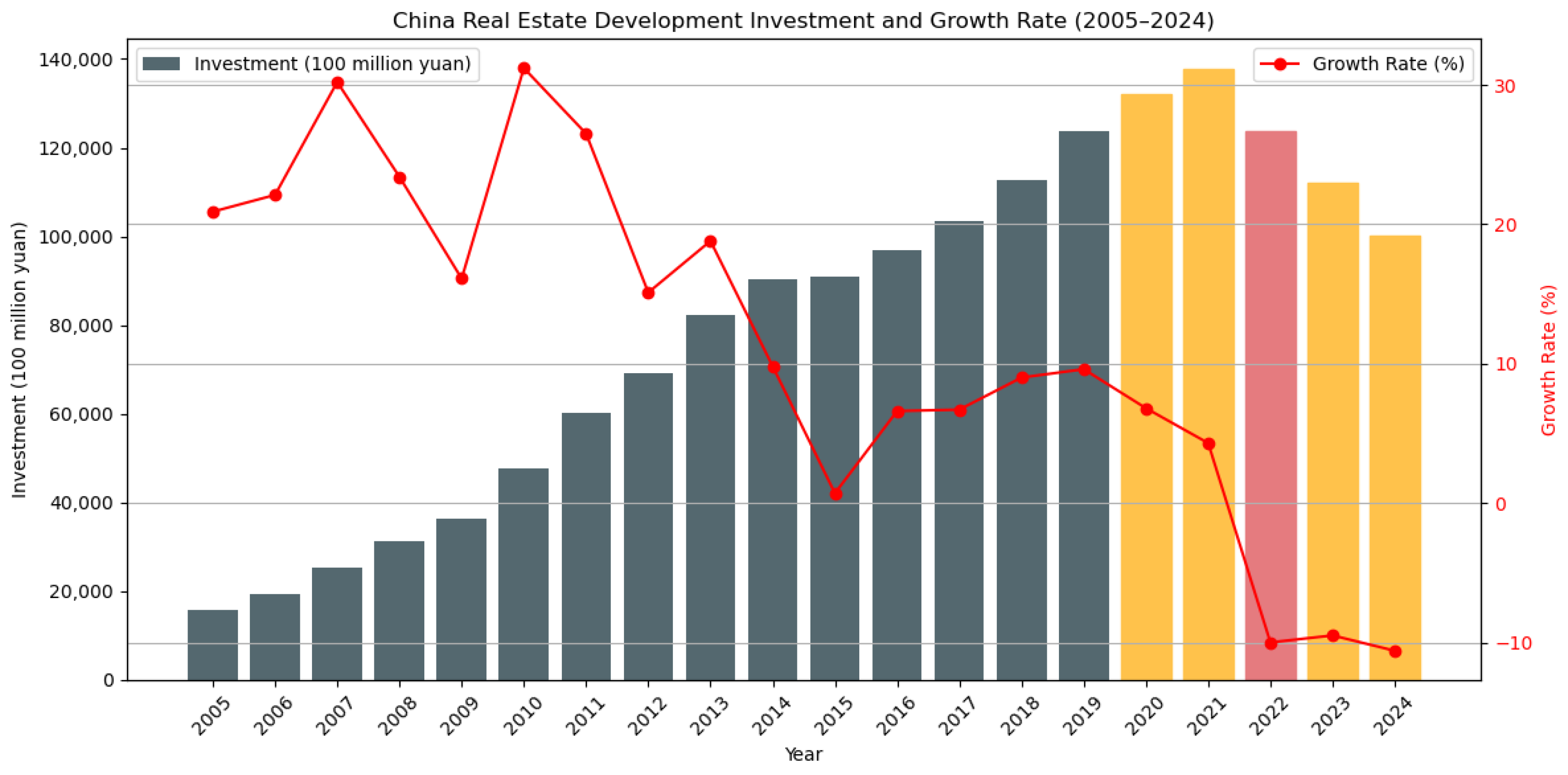
Guided by the growth rate of real estate development investment, as reported by the National Bureau of Statistics of China (see Figure 11), we focus our analysis on the period from 2020 to the present. A total of 740 stocks are included in the index over the sample period. Furthermore, we collect their daily return data from 5 June 2014 to 31 December 2019 for the purpose of constructing and filtering the financial network as this period reflects a relatively stable and connected financial–real estate environment, ideal for network construction and structural inference.

For risk forecasting, we employ daily data from 7 February 2022, to 20 January 2023, and weekly data from 5 January 2020, to 27 February 2025. Since 2019, China’s real estate sector has experienced a prolonged deceleration, with investment growth rates declining steadily and turning negative in 2022. This downward trend persisted through 2024, hovering around −10%, thereby offering a realistic setting for evaluating the predictive capacity of the FoPDE model under systemic stress. At the daily frequency, we specifically target 2022, which is the first year when real estate investment growth turned negative, and it marks a potential structural inflection point. And to ensure data quality and consistency, stocks with more than 10% missing values are excluded. Following the application of the Granger causality test and Motif-8 structural filtering, 133 entities remain and are set as the nodes in the financial network.

3.2. Network Analysis and Clustering

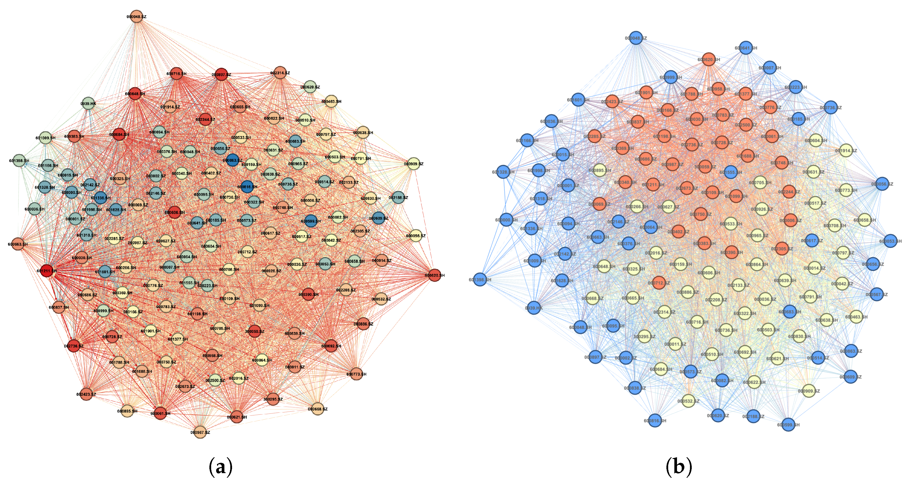
The resulting network comprises 11 banks—each among the 20 systemically important banks as identified in official Chinese documentation—alongside 44 non-bank financial institutions and 78 entities from the real estate and related sectors (see Figure 12a).

Following the methodologies outlined in Section 2.1.2, we filter the network and get $m=3$. Then, we partition the entities into three distinct clusters (see Figure 12b and

Table 2. Constituent stocks of each cluster.

Cluster 1		Cluster 2		Cluster 3
000712.SZ	601099.SH	000532.SZ	000797.SZ	000001.SZ	000838.SZ
601198.SH	601377.SH	000668.SZ	000926.SZ	000048.SZ	600663.SH
601211.SH	000783.SZ	600621.SH	000011.SZ	600095.SH	000056.SZ
000166.SZ	000069.SZ	000965.SZ	600266.SH	600641.SH	000567.SZ
002736.SZ	000750.SZ	600510.SH	600658.SH	000897.SZ	0939.HK
000987.SZ	000686.SZ	600533.SH	600864.SH	000002.SZ	600599.SH
600383.SH	002500.SZ	600736.SH	600503.SH	000573.SZ	000736.SZ
600369.SH	600390.SH	002016.SZ	600622.SH	600064.SH	600185.SH
600837.SH	002423.SZ	600716.SH	600638.SH	600082.SH	600376.SH
600340.SH	600748.SH	600773.SH	600648.SH	600094.SH	000617.SZ
601901.SH	002305.SZ	600692.SH	600705.SH	601555.SH	000863.SZ
600109.SH	000402.SZ	000036.SZ	000014.SZ	601628.SH	002142.SZ
600030.SH	600620.SH	000886.SZ	000631.SZ	600999.SH	600015.SH
000006.SZ	002285.SZ	300295.SZ	001914.SZ	000609.SZ	601009.SH
601788.SH	002673.SZ	600159.SH	600463.SH	002188.SZ	601166.SH
000728.SZ	601688.SH	600322.SH	000042.SZ	600053.SH	601318.SH
000776.SZ	002244.SZ	600325.SH	000627.SZ	600223.SH	601998.SH
300059.SZ	600061.SH	600639.SH	600604.SH	600816.SH	600036.SH
600958.SH	–	600665.SH	600791.SH	000514.SZ	600000.SH
–	–	600708.SH	600830.SH	000656.SZ	601398.SH
–	–	000517.SZ	600895.SH	600007.SH	600048.SH
–	–	600606.SH	002133.SZ	600683.SH	601328.SH
–	–	000909.SZ	002314.SZ	000620.SZ	601336.SH
–	–	600684.SH	002208.SZ	002146.SZ	601601.SH

). Cluster 1 contains the highest number of non-bank financial institutions, predominantly brokers and securities firms, accounting for approximately 70% of Cluster 1. Cluster 2 includes 40 of the 48 nodes identified as real estate entities, out of a total of 74 in the entire network. Cluster 3 is characterized by the inclusion of 10 out of the 11 banks, along with some large-scale entities of the financial and real estate sectors. A summary of the industry composition across all three clusters is provided in

Table 3. Industry composition of each cluster.

Cluster	Real Estate	Finance	SI Banks	Others
Cluster 1	10	26	1	0
Cluster 2	40	6	0	2
Cluster 3	24	12	10	2

Note: SI (Systemically Important) banks listed here are based on the official list of systemically important banks in China, published jointly by the People’s Bank of China (PBoC) and the National Financial Regulatory Administration (NFRA).

.

3.3. Risk Contagion in China’s Financial System

With reference to our previous work [22] and the methods introduced in Section 2.2, we calculate the relative distance among the clusters in

Table 4. Cluster distance analysis.

Cluster Pair	Sum of Weights	Distance
Cluster 1-2	340.804	0.595919
Cluster 2-3	282.406	0.665160
Cluster 1-3	220.195	0.738921

Note: Distance is calculated using the formula $d_{ij}=1-{\displaystyle \frac{w_{ij}}{{\omega }_{12}+{\omega }_{23}+{\omega }_{13}}}$, where $w_{ij}$ is the sum of edge weights between nodes in cluster i and cluster j.

.

While Table 4 shows that the Cluster 1–3 distance (0.738921) is not negligible in absolute terms, it represents the weakest relationship among all cluster pairs, being 24% and 11% more distant than the 1–2 and 2–3 relationships, respectively. Given the distinct operational characteristics of Cluster 1 (capital-market entities) and Cluster 3 (systemically important banks), we hypothesize that risk transmission occurs predominantly through the mediated pathway Cluster 1→2→3 rather than direct contagion. This assumption is consistent with financial network theory and allows for a more parsimonious FoPDE formulation while preserving the essential risk dynamics.

Based on the relative distances, Table 2 and Table 3, and the averaged $\Delta CoVaR$ calculated in

Table 5. Descriptive statistics of daily $\Delta CoVaR$ in different clusters.

Cluster	Count	Mean	Std	Min	25%	50%	75%	Max
Cluster 1	237	2.27	0.63	1.42	1.81	2.04	2.56	4.04
Cluster 2	237	2.24	0.46	1.67	1.89	2.08	2.45	3.61
Cluster 3	237	2.13	0.54	1.34	1.74	1.93	2.35	3.80

, a clear image of risk evolution in China’s financial system emerges (see Figure 13). Institutions are divided into three clusters based on network structure and systemic risk characteristics.

Cluster 1, encompassing capital-market-oriented entities such as securities firms (27 out of 37) and highly leveraged real estate developers, represents the high-risk group. These institutions exhibit strong pro-cyclicality, sensitivity to asset price fluctuations, and high leverage levels. Volatility in financial markets may impair their balance sheets rapidly, and their activities, such as stock pledges, margin financing, or bond underwriting, form transmission channels that may propagate shocks across sectors.

Cluster 2 comprises medium-risk institutions, notably regional real estate developers (40 out of 48) and local financial firms. Their vulnerabilities stem from geographically concentrated exposures, reliance on non-standard financing, and limited access to diversified funding sources. While their individual systemic contribution may be modest, collective stress within this group could trigger broader economic feedback loops, especially via local financial ecosystems.

Cluster 3 includes low-risk but systemically important institutions, such as large commercial banks, insurers, and leading real estate developers. Although these entities are better capitalized and more diversified, their centrality in the financial system implies that distress could produce outsized macro-financial consequences. Furthermore, market perceptions of implicit government support may induce moral hazard and lead to risk underpricing. Our findings echo those in the paper [74] that non-state-owned real estate companies are more easily contagious for rural banks, followed by state-owned, or systematically important banks.

This risk-based cluster difference highlights that contagion in China’s financial system is unlikely to be homogenous. Instead, it flows through institutional inter-linkages, market dependencies, and geographical channels, requiring differentiated regulatory attention and targeted macro-prudential policies.

4. Results and Discussion

Fitting data at different temporal resolutions can reveal distinct characteristics of risk evolution and contagion dynamics. The appropriate temporal resolution may vary across markets and regions, reflecting heterogeneous mechanisms of risk transmission [75].

In this study, we examine risk contagion from both daily and weekly data. For daily returns, which align with the temporal resolution of the data used in network construction, we expect better forecasting performance. In contrast, weekly returns aggregate risk dynamics over longer intervals, making them more suitable for capturing event-driven effects that often unfold over extended periods, while also providing an additional layer of model validation by testing robustness to heteroskedasticity.

4.1. Prediction and Analysis on Daily Data

We begin by modeling risk contagion using daily return data spanning from 7 February 2022, to 20 January 2023, aiming to capture the high-frequency dynamics of systemic risk. $\Delta CoVaR$ calculated on a daily basis is plotted in Figure 14, and the statistical description of it is shown below in Table 5. Notably, the data exhibits pronounced spikes in systemic risk around March, July, and December of 2022, alongside substantial volatility throughout the period, highlighting the complexity of the risk environment, which poses significant challenges for accurate forecasting.

This distribution of institutions in clusters is highly informative, as it reflects underlying patterns of risk accumulation and aligns closely with the $\Delta CoVaR$ estimates for each cluster. Further analysis confirms that Cluster 1 has the highest average risk level, while Cluster 3 exhibits the lowest, aligning with our expectations.

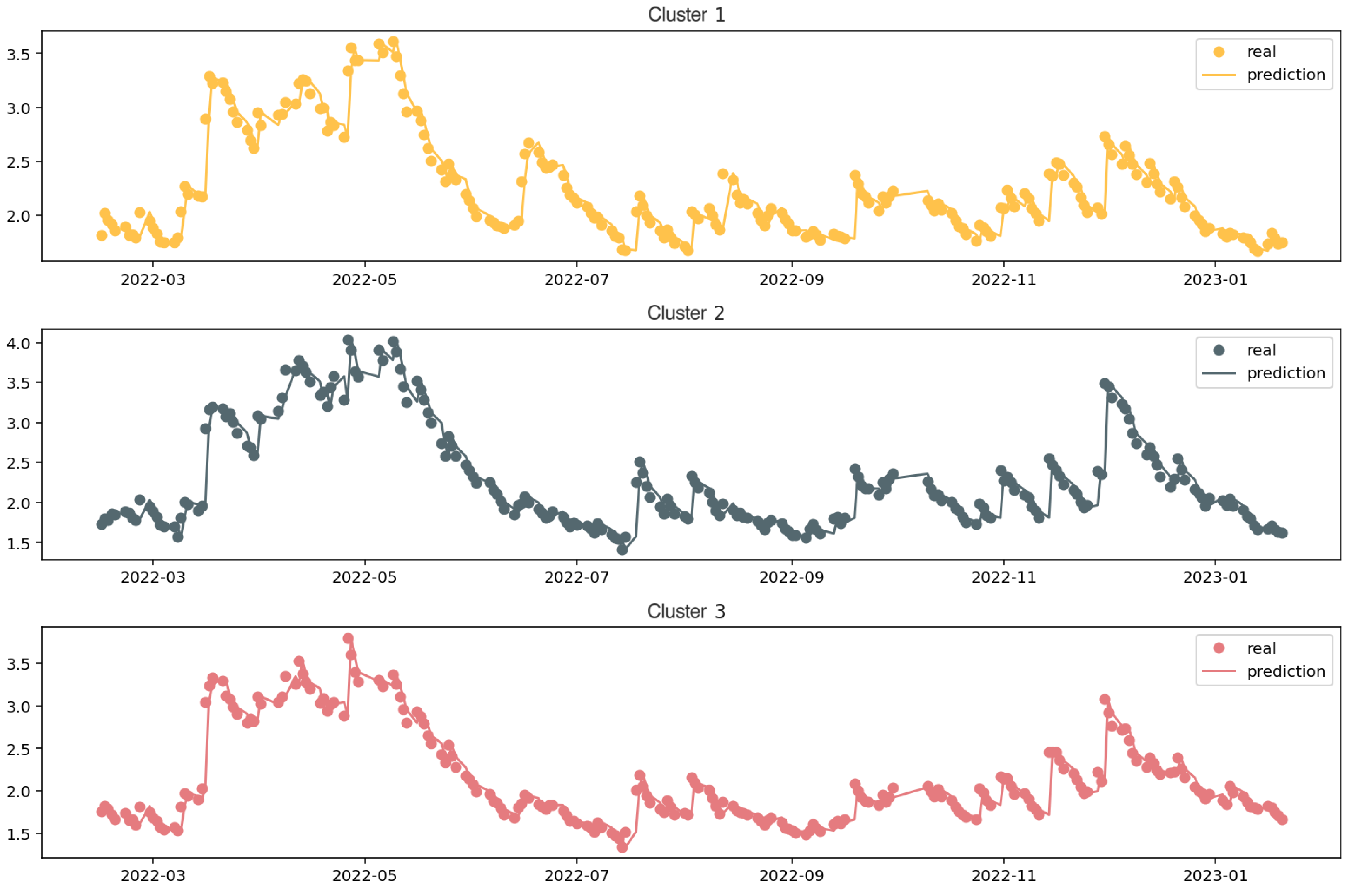
We adopt a sliding-window approach to fit the FoPDEs model. Specifically, with a window size of $L=10$, the model is trained on the preceding L observations to generate one-step-ahead forecasts. Owing to the structure of the model, we perform joint forecasting of the three interdependent time series that constitute the system. The result is shown below in Figure 15.

For performance assessment, we compare the performance of the proposed FoPDEs model against two established benchmarks in time-series forecasting: Long Short-Term Memory (LSTM) networks and Extreme Gradient Boosting (XGBoost).

The final performance metrics are reported in

Table 6. Error comparison of different prediction methods.

Method	MSE	MAE	MRE (%)	MRA (%)
FoPDEs	0.028706	0.106254	4.50	95.50
LSTM	0.032579	0.114770	5.00	95.00
XGBoost	0.031592	0.122121	5.34	94.66

* Model performance is evaluated using Mean Squared Error (MSE), Mean Absolute Error (MAE), Mean Relative Error (MRE), and MRA.

. Our FoPDEs model achieves a Mean Relative Accuracy (MRA) of 95.5%, the highest among the selected models, demonstrating strong performance across the periods of market fluctuations. The result highlights the model’s effectiveness in capturing the dynamics of complex financial systems and underscore its robustness under volatile conditions.

4.2. Prediction and Analysis on Weekly Data

Furthermore, we analyse the $\Delta \mathrm{CoVaR}$ derived from weekly return data spanning from 5 January 2020, to 27 February 2025. We perform forecasting modeling and examine the key patterns revealed in the corresponding figures. This empirical test of weekly data also serves as a heterogeneity test, evaluating the ability of the FoPDEs model to capture systemic risk dynamics across different temporal resolutions.

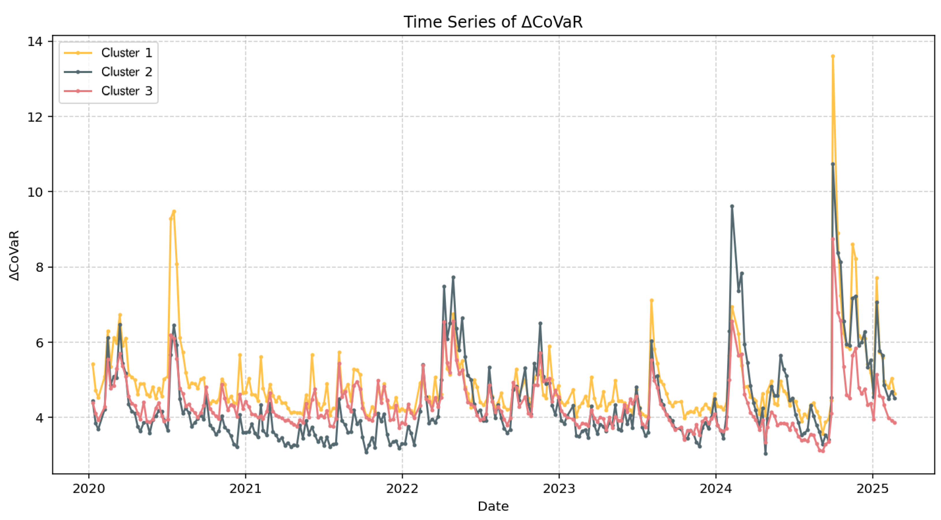
Weekly $\Delta CoVaR$ estimates are calculated and presented below in Figure 16, and the statistical description is provided in

Table 7. Descriptive statistics of weekly $\Delta CoVaR$ in different clusters.

Cluster	Count	Mean	Std	Min	25%	50%	75%	Max
Cluster 1	262	4.88	1.04	3.57	4.32	4.59	5.03	13.62
Cluster 2	262	4.36	1.14	3.04	3.63	3.98	4.61	10.74
Cluster 3	262	4.32	0.69	3.11	3.93	4.14	4.55	8.75

, revealing notable differences compared to the daily results. Specifically, the magnitude of the weekly $\Delta CoVaR$ tends to be larger than that of the daily data. For instance, when comparing the maximum values over the same period (March to June 2022), the peak of the daily $\Delta CoVaR$ reaches approximately 4, whereas the maximum value at the weekly resolution nearly doubles, approaching 8. This discrepancy suggests that risk accumulation and contagion effects are more pronounced when observed at lower-frequency data. Such findings are consistent with the notion that lower-frequency data may smooth out short-term fluctuations but amplify the aggregate impact of persistent shocks. Moreover, the weekly figures exhibit relatively fewer sharp spikes compared to the daily counterparts, reflecting the information aggregation effect induced by temporal resolution.

For weekly data, the performance of our model remains competitive across all error metrics. As shown in

Table 8. Error comparison of different prediction methods.

Method	MSE	MAE	MRE (%)	MRA (%)
FoPDEs	0.598838	0.421195	8.32	91.68
LSTM	0.502164	0.384774	7.82	92.18
XGBoost	0.693397	0.488036	9.75	90.25

, the FoPDEs model achieves a Mean Relative Accuracy (MRA) of 91.68%, closely comparable to the LSTM baseline at 92.18%, and outperforming XGBoost, which yields an MRA of 90.25%. This demonstrates the robustness of our approach in capturing patterns at lower temporal resolution while maintaining strong predictive accuracy.

These observations also provide a natural heterogeneity test for the FoPDEs model. Despite the differences in scale and dynamics between daily and weekly $\Delta CoVaR$ series, the FoPDEs model remains capable of capturing the underlying patterns of risk evolution. This suggests that the model is sufficiently flexible to accommodate varying temporal structures, thereby enhancing its applicability in risk prediction under different monitoring frequencies.

4.3. Event Study and Parameters Analysis

Furthermore, we attempt to capture the correlations between market events and $\Delta CoVaR$ and identify the possible patterns of how the fractional derivative parameter $\alpha$ changes in correspondence to different situations (see Figure 17).

A noteworthy pattern is observed in the behavior of the fractional order parameter $\alpha$. Specifically, $\alpha$ tends to decline when the $\Delta CoVaR$ rises and exhibits increased fluctuations. This phenomenon can be interpreted in light of the definition of the fractional derivative and fractional dynamics [76]: a lower value of $\alpha$ indicates that the model assigns greater weight to historical information, thereby increasing the system’s memory dependence. Such behavior reflects an inherent adaptive mechanism of our FoPDEs model, whereby the model places more emphasis on past observations when the system enters periods of heightened uncertainty. This is consistent with the notion that, under turbulent market conditions, recent data become more volatile and less informative for forward-looking risk estimation. Consequently, by dynamically adjusting the value of $\alpha$, the FoPDEs model is able to better adapt to structural changes, capture abrupt fluctuations, and enhance forecasting accuracy during periods of stress.

The results indicate that, in response to major shocks in the financial and real estate markets, the weekly $\Delta CoVaR$ demonstrates strong performance in capturing the onset of systemic risk cascades. Cases of events are labeled in Figure 17, proving that $\Delta CoVaR$ can largely reflect the risk contribution of the events to the system. Between February 2020 and October 2021, the COVID-19 pandemic triggered panic in the system and, during the late period of the pandemic, the intermittent lockdown measures and uneven recovery brought further uncertainty. Around March 2022, major real estate developer defaults, as exemplified by the Evergrande Real Estate Group, triggered systemic financial risk. Later, in the fourth quarter of 2022, the central government released the “three arrows” policy to ease risk in the real estate market. Commercial housing prices kept declining in 2023, resulting in dramatic fluctuation in the capital market. In September 2023, major policies were released by the government to stabilize the prices as well as the declining real estate market.

4.4. Recommendations for Policy

Building on the validation of empirical data, we now turn to potential measures that may mitigate risk contagion within the network.

First, early intervention based on temporal risk signals: The temporal dynamics of the model parameters reveal a pattern of risk accumulation preceding major systemic downturns. This observation justifies the incorporation of fractional-order derivative in the forecasting framework, as they effectively capture long-memory effects and latent risk build-up within the system. This mechanism also implies that early-stage interventions, which are triggered by the identification of rising systemic stress, could play a crucial role in mitigating the magnitude of future shocks, thereby enhancing the system’s overall resilience.

Second, de-financialization of the real estate sector: Cluster 1, which is identified as the segment with the highest systemic risk, is largely composed of non-bank financial institutions and local real estate developers. This suggests the necessity of reducing the financialization of the real estate sector. Limiting excessive speculative activity may help curb risk accumulation and contagion.

Third, strengthen resilience of core banking institutions: The empirical results underscore the pivotal role of banks in the network. As key risk-taking entities, banks not only channel capital to other participants but also absorb substantial systemic exposure. Therefore, maintaining the soundness and resilience of the banking sector is essential, particularly in the face of frequent and severe external shocks. Enhancing regulatory oversight and stress-testing frameworks could serve as effective tools to this end.

5. Conclusions

This paper integrates network analysis with Fractional-order Partial Differential Equations (FoPDEs) to model and forecast the evolution and contagion of systemic risk in financial networks.

For empirical validation, we use component stocks from China’s financial and real estate sectors, with data sourced from the WIND database. The model is applied to both daily and weekly return data and demonstrates strong predictive performance and robustness. Specifically, for daily data, the FoPDEs model achieves a Mean Relative Accuracy (MRA) of 95.5%, outperforming LSTM (95.0%) and XGBoost (94.7%). On a weekly basis, it maintains solid performance with an MRA of 91.7%. Notably, the estimated fractional order $\alpha$ tends to decrease during periods of rising risk, suggesting that the model captures the accumulation of systemic stress through long-memory effects. Based on these findings, we also propose several policy suggestions to enhance the robustness of the system.

The empirical results underscore the capacity of the FoPDEs framework to effectively model the dynamics of risk dynamics in complex financial systems. This approach not only achieves high predictive accuracy but also offers interpretability through its parameter structure, thereby providing a valuable tool for systemic risk analysis and policy design.