The Continued Fraction Structure in Physical Fractal Theory

Abstract

The objective of this study is to reveal the intrinsic connection between fractal operators in physical fractal spaces and continued fractions. The specific contributions include: (1) reviewing fundamental concepts of continued fractions and physical fractal theory; (2) establishing algebraic structure consistency between continued fractions and fractal operators through the medium of generation mappings; (3) discussing the convergence of fractal operators by employing theory from continued fraction analysis; and (4) confirming the correspondence between fixed points of infinite continued fractions and algebraic equations governing fractal operators.

1. Introduction

Continued fractions, originating from the Euclidean algorithm, are a mathematical concept dating back to ancient Greece. By applying the Euclidean algorithm, any rational number can be expressed as a continued fraction. Extending this method to irrational numbers leads to the emergence of infinite continued fractions. Between the 16th and 18th centuries, many irrational numbers were successfully represented in continued fraction form, including the most commonly used quadratic surd expansions [1].

With the advent of calculus in the 17th century, continued fractions were incorporated into the framework of mathematical analysis. Euler was the first to introduce continued fractions into analytical theory, establishing an equivalence between continued fractions and infinite series [2]. At this stage, continued fractions, much like series theory, evolved toward infinite non-periodic recursion. Gauss pioneered the study of continued fraction representations for functions, deriving expansions for both the hypergeometric function and the confluent hypergeometric function [3].

In the 19th century, Stieltjes approached the moment problem from the perspective of continued fractions, ultimately developing the renowned Stieltjes integral [4,5]. From the late 19th to the early 20th century, the convergence of continued fractions gained significant attention, leading to the formulation of widely applicable and concise convergence theorems [6,7].

The renowned Ramanujan also studied continued fractions during this period, proposing a series of astonishing continued fraction identities [8,9] and connecting them with elliptic functions [10] and modular forms [11]. His contributions remain highly influential in fields such as special functions [12] and number theory to this day [13,14].

During the mid to late 20th century, Soviet mathematicians expanded the concept of continued fractions, establishing the theory of branched continued fractions (BCFs) [15,16,17].

Today, continued fractions have become a powerful analytical tool. Due to their rapid convergence rate and algorithm-friendly computational process, they have been widely adopted in fields such as image recognition and machine learning. In engineering applications, continued fraction interpolation and Padé approximation based on continued fractions have found extensive use, with further extensions like vector-valued continued fraction interpolation being developed [18,19].

Moreover, continued fractions provide an effective approach for solving certain iterative recursion problems. For instance, they offer efficient solutions for Markov chains and birth–death processes, demonstrating superior computational advantages in these areas [20,21].

Physical fractal theory, an analytical method abstracted from biomechanical and physical research, represents a recently developed theoretical framework. This theory focuses on chain structures and their extensions, modeling physical processes as input–output systems where operators serve as the primary objects of study. Using circuit diagrams as auxiliary tools and employing key concepts such as fractal graphs, fractal cells, and fractal operators, it characterizes the intrinsic properties of corresponding processes. Ultimately, by applying operational calculus, the theory achieves a functional representation of operators, yielding convolution-type expressions for output quantities [22].

Currently, physical fractal theory has been successfully applied to diverse research areas, including hemodynamics [23]; bone mechanics [24]; and mineral seepage flows [25]. In each of these fields, the theory has demonstrated significant practical utility and achieved promising results.

Fractal operators, as mathematically defined mechanical concepts within physical fractal theory, serve as the operator-based representation of intrinsic quantities in mechanical processes. These operators lie at the core of physical fractal theory—indeed, grasping their essence equates to mastering the theory itself. Consequently, extensive research has been conducted on solution methods for fractal operators and their equivalent representations [26]. But it should be noted that existing studies primarily address the evaluated forms of fractal operators rather than their intrinsic mathematical structure, which remains to be fully elucidated.

These studies primarily exploit the infinite character of the fractal diagrams, which implies that any prospective subpart of the diagram or expression can be regarded as equivalent to the entire diagram itself. This allows the subpart (in all its recursively infinite structure) to be captured in a single algebraic variable—namely, the fractal operator.

This concept closely parallels the approach used in studying the “infinite telegraph line” or “infinite transmission line” problem, where the equivalent resistance of an infinite ladder resistor network is calculated. This problem is also known as the “golden transmission line” problem since its solution yields the Fibonacci golden ratio [27,28].

It is worth noting that continued fractions have also found applications in resistor network research. For instance, Isokawa demonstrated that the minimal circuit configuration for a given resistance value “w” inherently adopts a continued fraction form [29], while Perano derived the continued fraction representation for the equivalent resistance of finite-level ladder circuits [30].

However, both works stopped short of explaining the underlying origin of this connection—their results were derived procedurally rather than traced to first principles. Moreover, their analyses were confined to finite-term continued fractions, leaving the infinite case unexplored.

In physical fractals, the “fractal operator” originates from physical properties and is typically a non-rational operator involving differential operations. Its non-rational nature stems from the infinite hierarchy of the system. The fractal operator is independent of the system’s input and output, reflecting its intrinsic characteristics. It plays a pivotal role in studying the system’s fundamental properties. Therefore, the continued fraction structure of fractal operators investigated in this work holds far greater significance compared with previous studies on continued fraction representations of physical constants.

At first glance, continued fractions and fractal operators appear entirely unrelated—they belong to distinct disciplines with divergent origins and no obvious connection. However, our research reveals an unexpected and profound relationship between them. This paper employs comparative analysis to demonstrate their hidden linkages, illustrating that the fractal operator is an operator with a continued fraction structure. By leveraging the well-established theory of continued fractions, we aim to strengthen the logical foundation of the fractal operator, thereby further refining physical fractals—a highly promising analytical approach.

The structure of this paper is organized as follows: Section 2 provides a review of fundamental concepts related to continued fractions. Section 3 revisits physical fractal spaces and the fractal operators defined on them. In Section 4, we examine the unification between continued fractions and fractal operators through the lens of generating mappings. Finally, Section 5 investigates fractal operators using analytical tools from continued fraction theory, particularly focusing on convergence and fixed-point theorems.

2. Concepts Related to Continued Fractions

Following the logical framework established in Continued Fractions: Analytic Theory and Applications by W.B. Jones et al. [31], we systematically review and organize the fundamental concepts of continued fractions relevant to this study.

Definition 1.

A continued fraction is an ordered pair $<<\left\{a_n\right\},\left\{b_n\right\}>,\left\{f_n\right\}>$, where a₁, a₂, … and b₁, b₂, … are complex numbers with all a_n $\ne 0$ and where $\left\{f_n\right\}$ is a sequence in the extended complex plane defined as $f_n=S_n(0)$. $\left\{f_n\right\}$ is designated as the n-th convergent. S(w) is referred to as the convergent mapping, which satisfies $S_0(w)=b_0+w$ and $S_n(w)=S_{n-1}({\displaystyle \frac{a_n}{b_n+w}})$.

In addition to the ordered array representation given in Definition 1, continued fractions are commonly denoted equivalently by their convergent $f_n$ in mathematical literature. This convergent $f_n$ admits several standard notational forms, of which we present the three most prevalent variants below:

$$f_n=b_0+{\displaystyle \frac{a_1}{b_1+\frac{a_2}{b_2+\frac{a_3}{\begin{array}{l}\cdots \cdots \\ b_{n-1}+\frac{a_n}{b_n}\end{array}}}}}.$$

(1)

$$f_n=b_0+{\displaystyle \frac{a_1}{b_1}}+{\displaystyle \frac{a_2}{b_2}}+{\displaystyle \frac{a_3}{b_3}}+\dots +{\displaystyle \frac{a_n}{b_n}}.$$

(2)

$$f_n=b_0+\underset{k=1}{\overset{n}{K}}({\displaystyle \raisebox{1ex}{$a_k$}\!\left/ \!\raisebox{-1ex}{$b_k$}\right.}).$$

(3)

It is evident that the convergent $f_n$ is computable, and we define the computed result of $f_n$ as the value of the n-th-order convergent of the continued fraction. The nature of the sequence $\left\{a_n\right\},\left\{b_n\right\}$ in the ordered array determines the type of continued fraction: when $\left\{a_n\right\},\left\{b_n\right\}$ constitutes a finite sequence, the corresponding continued fraction has finite terms and is called a finite continued fraction; whereas when $\left\{a_n\right\},\left\{b_n\right\}$ is an infinite sequence, it generates an infinite continued fraction.

For finite continued fractions, convergents provide exact representations of their actual values. However, for infinite continued fractions, the value cannot be precisely expressed by a finite convergent—any truncation at a finite term inevitably introduces a remainder term, which corresponds to the familiar concept of approximation error. Nevertheless, we can formally extend the concept of the convergent to infinity in a limiting sense.

Definition 2.

The value of an infinite continued fraction $b_0+\underset{n=1}{\overset{\infty }{K}}({\displaystyle \raisebox{1ex}{$a_n$}\!\left/ \!\raisebox{-1ex}{$b_n$}\right.})$ is denoted as f, where $f=\underset{n\to \infty }{\lim }{f}_n$.

We can equivalently express the value of an infinite continued fraction through its convergent mapping, yielding Equation (4):

$$f=\underset{n\to \infty }{\lim }{\left.S_n(w)\right|}_{w=0}.$$

(4)

In physical fractal theory, the fundamental assumption of infiniteness inherently leads to corresponding continued fractions that are infinite in nature. Therefore, for the sake of analytical convenience, we hereby establish the convention that all subsequent references to continued fractions in this work, unless otherwise specified, shall denote infinite continued fractions.

While discussions based on convergents often adopt a truncation-based perspective, an alternative approach examines the continued fraction’s term-by-term construction process from the bottom up. From this viewpoint, a continued fraction can be interpreted as a nested sequence of fractional mappings—collectively referred to as generating mappings.

Definition 3.

The sequence of mappings $\{t_n(w)\}$ satisfying $t_0(w)=b_0+w$ and $t_n(w)={\displaystyle \frac{a_n}{b_n+w}}$ is termed the generating mapping sequence, and $t_n(w)$ is referred to as the n-th generating mapping.

Obviously, according to the definition of convergent mapping, the result of sequentially combining the first n generating mappings is the n-th convergent mapping. Correspondingly, the value of the continued fraction admits a representation via this composition, expressed in the language of a formula as follows.

Theorem 1.

$S_n(w)=t_n\circ t_{n-1}\circ \dots \circ t_1\circ t_0(w)$, $f=\underset{n\to \infty }{\lim }{\left.t_n\circ t_{n-1}\circ \dots \circ t_1\circ t_0(w)\right|}_{w=0}$.

When all terms in the generating mapping sequence are identical, the nested composition simplifies to a compact power form:

Corollary 1.

$S_n(w)=t^n(w)$, $f=\underset{n\to \infty }{\lim }{\left.t^n(w)\right|}_{w=0}$.

A given value may admit multiple distinct continued fraction expansions, thereby establishing an equivalence relation among these structures. Leveraging such equivalence transformations often yields significant simplifications in analytical investigations. As a specific method to enhance representational efficiency, we will later employ contraction of continued fractions.

Definition 4.

Let $\left\{f_n\right\}$ be the sequence of convergent for the continued fraction $b_0+\underset{n=1}{\overset{\infty }{K}}({\displaystyle \raisebox{1ex}{$a_n$}\!\left/ \!\raisebox{-1ex}{$b_n$}\right.})$ and $\left\{f_n^{*}\right\}$ the convergent for $b_0^{*}+\underset{n=1}{\overset{\infty }{K}}({\displaystyle \raisebox{1ex}{$a_n^{*}$}\!\left/ \!\raisebox{-1ex}{$b_n^{*}$}\right.})$. If $\left\{f_n^{*}\right\}$forms a subsequence of  $\left\{f_n\right\}$, then $b_0^{*}+\underset{n=1}{\overset{\infty }{K}}({\displaystyle \raisebox{1ex}{$a_n^{*}$}\!\left/ \!\raisebox{-1ex}{$b_n^{*}$}\right.})$ is called a contraction of $b_0+\underset{n=1}{\overset{\infty }{K}}({\displaystyle \raisebox{1ex}{$a_n$}\!\left/ \!\raisebox{-1ex}{$b_n$}\right.})$.

Commonly used contractions include odd contraction and even contraction, whose convergent sequences satisfy conditions $f_n^{*}=f_{2n+1}$ and $f_n^{*}=f_{2n}$, respectively. We state these two theorems without proof.

Theorem 2.

When $b_{2k}\ne 0$, continued fraction $b_0+\underset{n=1}{\overset{\infty }{K}}({\displaystyle \raisebox{1ex}{$a_n$}\!\left/ \!\raisebox{-1ex}{$b_n$}\right.})$ with convergent mapping $S_n(w)={\displaystyle \frac{a_n}{b_n+w}}$ has an even contraction $b_0^{*}+\underset{n=1}{\overset{\infty }{K}}({\displaystyle \raisebox{1ex}{$a_n^{*}$}\!\left/ \!\raisebox{-1ex}{$b_n^{*}$}\right.})$, satisfying:

$$b_0^{*}=b_0, a_1^{*}=a_1{b}_2, b_1^{*}=a_2+b_1{b}_2, a_2^{*}=-a_2{a}_3{b}_4,$$

$$a_k^{*}=-a_{2k-2}{a}_{2k-1}{b}_{2k-4}{b}_{2k},b_k^{*}=a_{2k-1}{b}_{2k}+b_{2k-2}(a_{2k}+b_{2k-1}{b}_{2k}).$$

Theorem 3.

When $b_{2k+1}\ne 0$, continued fraction  $b_0+\underset{n=1}{\overset{\infty }{K}}({\displaystyle \raisebox{1ex}{$a_n$}\!\left/ \!\raisebox{-1ex}{$b_n$}\right.})$ with convergent mapping  $S_n(w)={\displaystyle \frac{a_n}{b_n+w}}$ has an odd contraction $b_0^{*}+\underset{n=1}{\overset{\infty }{K}}({\displaystyle \raisebox{1ex}{$a_n^{*}$}\!\left/ \!\raisebox{-1ex}{$b_n^{*}$}\right.})$, satisfying: $a_1^{*}=-{\displaystyle \frac{a_1{a}_2{b}_3}{b_1}}$, $b_1^{*}=a_2{b}_3+b_1(a_3+b_2{b}_3)$, $a_k^{*}=-a_{2k-1}{a}_{2k}{b}_{2k-3}{b}_{2k+1}$, and $b_k^{*}=a_{2k}{b}_{2k+1}+b_{2k-1}(a_{2k+1}+b_{2k}{b}_{2k+1})$.

When the sequence $\left\{a_n\right\},\left\{b_n\right\}$ exhibits periodicity, the structure of the continued fraction can be substantially simplified. This simplified form is conventionally termed a periodic continued fraction.

Definition 5.

When $a_{rm+k}=a_k$ and  $b_{rm+k}=b_k(r,m\in N)$, the continuous fraction  $\underset{n=1}{\overset{\infty }{K}}({\displaystyle \raisebox{1ex}{$a_n$}\!\left/ \!\raisebox{-1ex}{$b_n$}\right.})$ is called a periodic continued fraction with period m.

It is straightforward to observe that the application of Theorems 3 and 4 to periodic continued fractions carries significant implications. Specifically, this contraction transformation can reduce the original period length by exactly half.

Periodic continued fractions represent the earliest and most thoroughly studied class of continued fractions in mathematical history. As early as the 18th century, Lagrange established a pivotal theorem in the theory of periodic continued fractions [32].

Theorem 4.

There exists a constructive isomorphism between the set of real quadratic irrationals and the class of periodic continued fractions.

Since every real quadratic irrational can be expressed as the root of a monic quadratic equation, Lagrange’s theorem essentially establishes a fundamental link between periodic continued fractions and quadratic equations. This connection was later recognized to arise through fixed-point equations.

Specifically, the value of a continued fraction coincides precisely with the fixed point of its associated contraction mapping. Thus, solving the fixed-point equation is equivalent to evaluating the continued fraction. However, the existence of such an equation inherently depends on the existence of the fixed point—that is, the continued fraction must converge to a well-defined value. This imposes strict requirements on the convergence properties of the continued fraction.

We therefore introduce the convergence theorem for continued fractions. It should be noted that general convergence theorems tend to be overly complex for our current discussion. For clarity and practicality, we have selected a more specific yet significantly simpler convergence theorem that better serves our purposes.

Theorem 5.

The periodic continued fraction $K({\displaystyle \raisebox{1ex}{$a$}\!\left/ \!\raisebox{-1ex}{$1$}\right.})$ converges to w₁ for all non-zero complex numbers a unless  $a={\displaystyle \raisebox{1ex}{$-1$}\!\left/ \!\raisebox{-1ex}{$4$}\right.}+c$, where c is real and negative. For $a={\displaystyle \raisebox{1ex}{$-1$}\!\left/ \!\raisebox{-1ex}{$4$}\right.}+c$, $c=\left|c\right|e^{i\gamma }$, $-\pi <\gamma <\pi$, the value of  $K({\displaystyle \raisebox{1ex}{$a$}\!\left/ \!\raisebox{-1ex}{$1$}\right.})$  is $w_1={\displaystyle \frac{-1+2\sqrt{\left|c\right|}{e}^{\raisebox{1ex}{$i\gamma $}\!\left/ \!\raisebox{-1ex}{$2$}\right.}}{2}}$.

This theorem is undoubtedly derived from general convergence theorems, with its complete derivation process being detailed in Reference [31]. The term w₁ introduced in the theorem represents a novel concept, which we now define as follows:

Definition 6.

The attractive fixed point of a function f(x) is a point x* satisfying f(x*) = x* and

$$\exists \delta >0, \forall x\in U(x^{*}, \delta ), \exists N\in N^{*} \mathit{\text{s.t.}} \forall n>N, \left|f^n(x)-x^{*}\right|<\delta .$$

The repulsive fixed point of a function f(x) is a point x* satisfying f(x*) = x* and

$$\exists \delta >0, \forall x\in U(x^{*}, \delta ), \exists n\in N^{*} \mathit{\text{s.t.}} \left|f^n(x)-x^{*}\right|\ge \delta .$$

Mathematicians have long established a universal method for determining fixed-point types, which can be readily derived from the contraction mapping principle. The proof of this theorem is so fundamental that it frequently appears as an exercise in calculus textbooks.

Theorem 6.

For the fixed point x*of the function f(x), if |f″(x)| < 1, then x* is attractive; if |f*′(x)| > 1, then x* is repulsive.

Thus, we have completed our discussion of the fundamental theory of continued fractions in the context of fractal operators.

3. Introduction to Physical Fractal Theory

Physical fractal structure is a topological structure formed by interconnected physical components, abstracted from real biological architectures and movements within living organisms. For instance, the fractalization of force and deformation transmission in tendon fiber mechanics naturally leads to such physical fractal structures, as illustrated in Figure 1 [22]. The key steps of this fractalization process are as follows:

(1) Selecting tendon microfibrils as the research subject, and benefiting from the tendon’s inherent hierarchical self-similar fractal structure, we can readily extrapolate the properties obtained from microfibril-level studies to macroscopic tendon behavior.

(2) Treating the microfibril ensemble as the research subject, we model it as a bundled assembly of molecular chains, where each chain consists of collagen molecules embedded within a gel matrix.

(3) Isolating a single molecular chain as the research subject, we employ infinitesimal decomposition to conceptualize the finite-length chain as an infinite series of collagen molecules connected end-to-end.

(4) At the collagen level, force–deformation transmission is decomposed into elastic deformation of collagen molecules and shear-lag effects from collagen–gel matrix interactions.

Using electromechanical analogy:

• ▪ Elastic deformation → Spring element (T₁);
• ▪ Shear-lag → Dashpot element (T₂);
• ▪ Adjacent unit effects → Hierarchical element (T).

Circuit topology is determined by force–deformation transmission pathways along the linear chain, yielding a single unit’s equivalent circuit model.

(5) Recursively substituting the hierarchical element with identical units through this generation rule constructs the physical fractal structure observed in tendon fibrils.

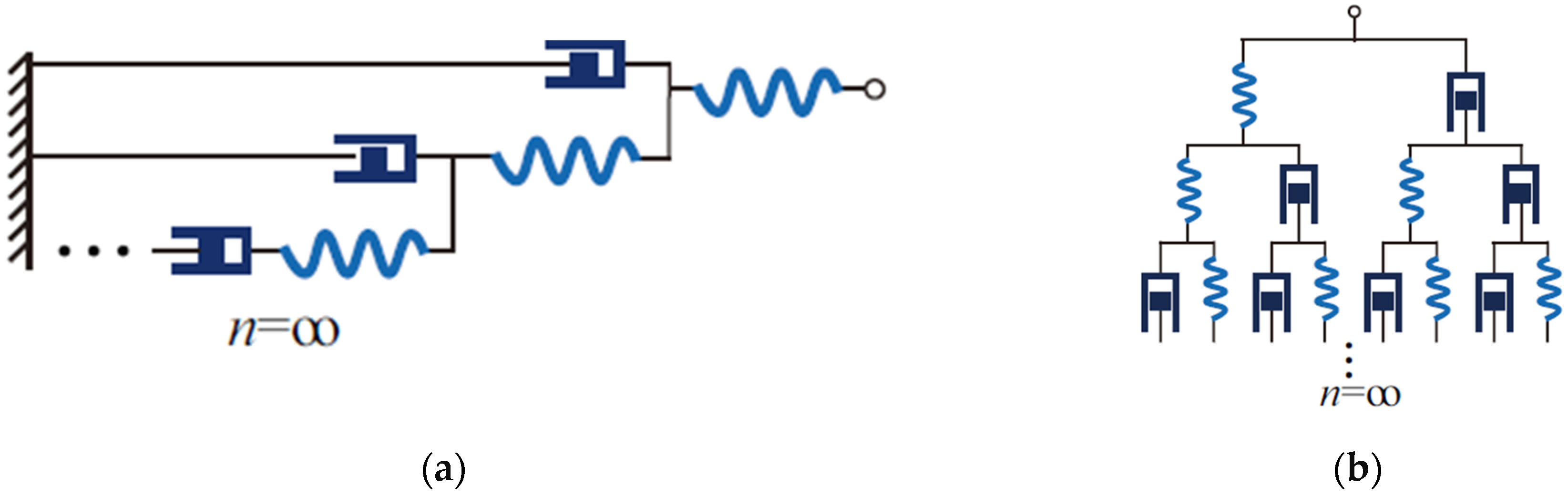
It should be noted that this abstraction approach is universal, and consequently, it induces distinct physical fractal structures for different physical systems [23,24,25]. Among various types of physical fractal spaces, tree-like fractals are the most common. These can be classified into two fundamental forms—symmetric fractal trees and fractal ladders [26].

For clarity, we focus on fractal ladders to revisit key concepts in physical fractal spaces. A fractal ladder is a symmetry-broken variant of a fractal tree. As illustrated in Figure 2a, compared with the perfectly symmetric fractal tree in Figure 2b, the fractal ladder exhibits broken symmetry due to its dashpot component being directly connected to the base node.

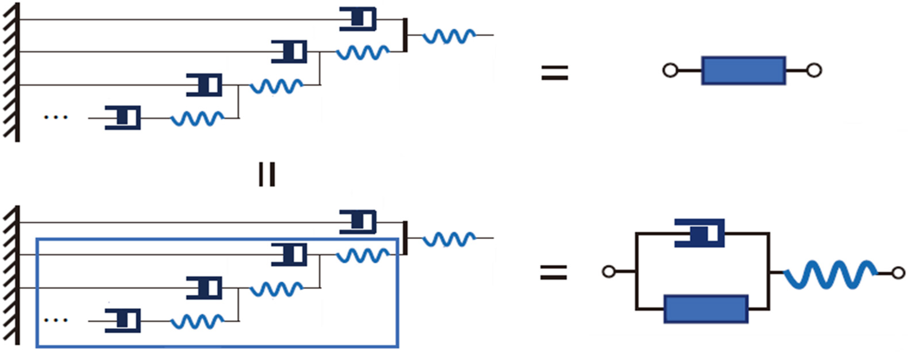
The workflow of physical fractal theory is illustrated in Figure 3a–d. Figure 3a displays the topological equivalent diagram of a single-unit cell. By connecting an identical unit cell to Figure 3a following specific linking rules, we obtain a second-order equivalent diagram as Figure 3b shows. Both the unit cell’s topological representation and the linking rules are abstracted from actual physical processes and are problem-dependent.

By the identity hypothesis of physical fractal theory, all unit cells and their linking rules remain invariant across hierarchical levels. Thus, the construction method from Figure 3a to Figure 3b generalizes to arbitrary-order equivalent diagrams. To increase the hierarchical order, we append identical unit cells to the existing diagram under the same linking rules. This stepwise extension is termed an iteration.

The physical fractal theory posits that real-world processes correspond to infinite-order structures. Hence, the topological diagram Figure 3c—obtained by applying infinite iterations to the single-unit diagram Figure 3a—represents the actual physical system and is called the fractal diagram. Crucially, all hierarchical substructures in Figure 3c are identical, manifesting the theory’s foundational property of self-similarity.

The fractal unit cell Figure 3d represents a further abstraction of the fractal diagram Figure 3c, where the infinite-order structure of Figure 3c is simplified into a single equivalent component by defining a holistic fractal element (as shown in Figure 4) that is functionally identical to the entire fractal diagram Figure 3c. This simplification relies fundamentally on the hypothesis of infinite self-identity. As illustrated in Figure 4, we enclose all structures of the fractal diagram Figure 3c except the first-level unit within a dashed boundary—this enclosed structure corresponds to an (n − 1)-order configuration. However, due to the nature of infinity, adding or subtracting finite terms does not alter its cardinality, meaning the enclosed structure remains an n-order system. Consequently, the content within the dashed boundary is structurally identical to the full fractal diagram Figure 3c. By defining this enclosed structure as the holistic fractal element and performing a substitution, we derive the fractal unit cell Figure 3d.

By leveraging the equivalence between the fractal unit cell and the fractal diagram Figure 3c, we can use the locality of the unit cell to characterize the global system. The construction of the fractal diagram Figure 3c from the fractal unit cell follows a straightforward process: as a generalized extension of the unit cell, this procedure is structurally identical to building Figure 3c from the original unit cell, except that the iterative process now replaces all holistic fractal elements in the existing structure with fractal unit cells. This reveals that the holistic fractal element is essentially an explicit manifestation of the unit cell’s linking rules.

However, the topological diagram representation of physical fractal concepts remains concrete. To enable analytical computations, we must introduce operator-theoretic formulations. The transformation between these two representations is achieved through valuation of the topological diagrams. Due to the universality of this valuation process, the entire physical fractal theory maintains complete symmetry. We can exploit this symmetry to significantly simplify our analysis.

The value of the fractal diagram Figure 3c is defined as the fractal operator, denoted by T. As an operator encoding global system properties, solving for T is equivalent to solving the original physical problem, making it the cornerstone of physical fractal theory. Obviously, since the holistic fractal element is functionally equivalent to the full fractal diagram Figure 3c, its value must also be the fractal operator T.

As finite truncations of the fractal diagram, the values of equivalent diagrams Figure 3a,b naturally approximate the fractal operator T, typically termed the n-th-order convergent. The fractal unit cell exhibits unique behavior: through its embedded holistic fractal element, its value inherently incorporates the fractal operator T itself. Crucially, since T cannot be explicitly determined from the unit cell alone, it functionally becomes a definite yet unknown quantity within this framework. Such expressions containing unresolved operators are systematically treated as mappings—thus, the fractal unit cell fundamentally represents a mapping t(w) of T rather than a conventional operator. This mapping is formally designated as the generating mapping.

The construction process from fractal unit cells to the complete fractal diagram Figure 3c admits an elegant representation through this mapping perspective. Here, the iterative substitution of holistic fractal elements with unit cells translates mathematically into recursive self-application of the mapping, where the independent variable becomes the mapping itself. This iterative procedure manifests as functional self-composition, yielding a fundamental definition:

Definition 7.

The value of the fractal diagram is termed the fractal operator, denoted as T, which satisfies $\underset{n\to \infty }{\lim }{\left.t^n(w)\right|}_{w=0}=T$, where t(w) represents the generating mapping.

4. The Hidden Continued Fraction Structure in Generating Mappings

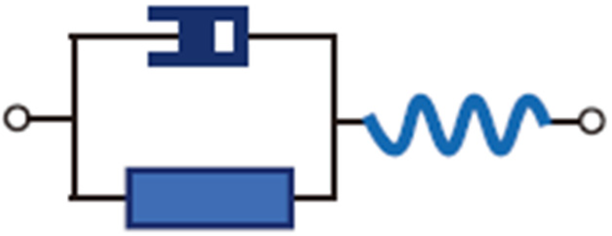
Classical continued fractions, as algebraic structures, are purely mathematical concepts devoid of physical imagery. Remarkably, we have recently identified a physical representation in continued fraction form, which directly correlates with concepts in physical fractal theory. This continued-fraction-based physical representation manifests in the most classical bifurcated fractal ladder structures. By substituting the definitions of physical fractal space concepts from the preceding section into these specific configurations, we obtain their concrete mathematical representations.

We analyze the unit cell diagram of the fractal ladder (Figure 5), evaluating its components by assigning:

• w: value of the holistic fractal element (a definite yet unknown quantity);
• a: constant value of the spring operator;
• b: constant value of the dashpot operator.

It is evident that here, for the sake of discussion, a and b are taken to represent the operators corresponding to springs and dashpots, respectively. However, in reality, a and b can denote the operators of any components, such as capacitors, inductors, or other elements involving differential operations, as discussed in References [23,24,25].

The prerequisite for our subsequent operator analysis lies in our prior proof that the operator domain and the number field exhibit a certain isomorphic relationship, ensuring consistency in their algebraic operation rules [33].

The operational rules for the electromechanically equivalent topological diagram are as follows:

$$\begin{gathered} \text{Parallel connection:} P(T_1, T_2)=T_1+T_2. \\ \text{Series connection:} S(T_1, T_2)={\displaystyle \frac{1}{\frac{1}{T_1}+\frac{1}{T_2}}}. \end{gathered}$$

(5)

The value of the fractal unit cell is given by:

$$t(w)=S(a, P(b,w))={\displaystyle \frac{1}{\frac{1}{a}+\frac{1}{b+w}}}.$$

(6)

Clearly, this represents a mapping with respect to w. Equation (6) is precisely the generating mapping of the fractal ladder. By substituting this generating mapping into Definition 7, we can solve for the fractal operator.

By substituting term by term and expanding, we obtain the explicit representation of T:

$$T={\displaystyle \frac{1}{\raisebox{1ex}{$1$}\!\left/ \!\raisebox{-1ex}{$a$}\right.+\frac{1}{b+\frac{1}{\raisebox{1ex}{$1$}\!\left/ \!\raisebox{-1ex}{$a$}\right.+\frac{1}{b+\dots }}}}}={\displaystyle \frac{1}{\raisebox{1ex}{$1$}\!\left/ \!\raisebox{-1ex}{$a$}\right.}}+{\displaystyle \frac{1}{b}}+{\displaystyle \frac{1}{\raisebox{1ex}{$1$}\!\left/ \!\raisebox{-1ex}{$a$}\right.}}+{\displaystyle \frac{1}{b}}+\dots .$$

(7)

This is exactly a periodic continued fraction with period 2.

Evidently, the fractal operator of a bifurcated fractal ladder is an operator expressed in continued fraction form, while the bifurcated fractal ladder itself represents the physical process corresponding to this continued fraction. Continued fractions thus serve as the intrinsic language for describing bifurcated physical fractal processes.

This correspondence is no coincidence but stems from the foundational definitions linking continued fractions with physical fractal concepts. For a periodic continued fraction with period k, its generating mapping also forms a periodic sequence with period k. We can always reduce these k mappings to an equivalent single mapping, thereby simplifying the periodic mapping sequence into an identical mapping sequence. Consequently, the periodic continued fraction can be expressed as a structure generated through infinite nested iterations of this single mapping.

Correspondingly, the most fundamental characteristic of physical fractals—self-congruence—is likewise the result of repeated iterations of such a single mapping. From a general perspective, both fractal diagrams and fractal operators can be viewed as outcomes of infinitely nested iterations of elementary unit cells and their generating mappings. This consistency in constructive philosophy fundamentally ensures the profound connection between the two.

However, the actual correspondence still requires concrete formal derivation. Clearly, algebraic-form continued fractions and topological-form fractal diagrams cannot be unified in representation, thus precluding any direct equality. As fractal operators satisfy algebraic operations and share formal consistency with continued fractions, they emerge as potential equivalent candidates.

Since the construction of the final global structure stems from nested iterations of fundamental mappings, consistency in the basic mapping form guarantees consistency in the resultant structure. Thus, the problem reduces to whether the generating mapping sequence of the fractal ladder can be expressed as a composition of Möbius transformations. During the valuation of topological diagrams, component values participate only as operands in operations determined solely by series-parallel rules. Provided these rules adhere to Möbius transformations, the fractal operator inherently possesses a continued fraction structure.

Since addition can be considered a degenerate case of Möbius transformations, it becomes evident that series-parallel rules inherently satisfy the required conditions.

Consequently, we arrive at the following conclusion: the continued fraction structure in fractal ladders originates from the series-parallel rules governing their topological diagrams, while the coefficients of the continued fraction derive from the component values within these diagrams.

This correspondence between algebraic structure and topological operational rules can be further generalized. By extending the fractal ladder model beyond the configuration shown in Figure 2a, we consider cases where components at different hierarchical levels lose their identical properties while maintaining the same series-parallel rules as specified in Equation (5).

Let us denote the values of spring components at successive levels as sequence {a_n} and dashpot components as sequence {b_n}. Although the components are no longer identical across levels, the ladder’s topological invariance persists due to its retained stepwise structure. This allows us to continue using unit cell analysis, albeit with generalized unit cells where component values become variable rather than fixed.

We immediately obtain the generating mapping as:

$$t_n(w)={\displaystyle \frac{1}{\frac{1}{a_n}+\frac{1}{b_n+w}}}.$$

(8)

Note that in this case, the generating mappings are no longer identical but appear as a sequence of mappings {t_n(w)}. However, since the iterative process of the unit cell is still represented by mapping composition, Definition 7 should be revised as follows:

$$\underset{n\to \infty }{\lim }{\left.t_n\circ t_{n-1}\circ \dots \circ t_1\circ t_0(w)\right|}_{w=0}=T.$$

(9)

Comparing with generating mapping theorems in continued fractions:

$$S_n(w)=t_n\circ t_{n-1}\circ \dots \circ t_1\circ t_0(w), f=\underset{n\to \infty }{\lim }{\left.t_n\circ t_{n-1}\circ \dots \circ t_1\circ t_0(w)\right|}_{w=0}.$$

(10)

It becomes evident that the fractal operator is essentially the value of a continued fraction. However, unlike the classical fractal ladder case, which exhibits higher symmetry (resulting in more symmetric periodic continued fractions), the generalized case breaks the component identity symmetry and consequently yields less symmetric, general continued fraction structures.

Remarkably, we can freely define the series-parallel rules in the circuit diagram to modify the corresponding algebraic structure. Here, we provide just one illustrative example.

Let us define the series-parallel rules as:

$$\begin{gathered} \text{Parallel connection:} P(T_1,T_2)=\sqrt{T_1+T_2}. \\ \text{Series connection:} S(T_1,T_2)=T_1+T_2. \end{gathered}$$

(11)

The fractal unit cell has a value of:

$$t(w)=S(a,P(b,w))=a+\sqrt{b+w}.$$

(12)

Through term-by-term substitution and subsequent expansion, we derive the explicit expression for T:

$$T=a+\sqrt{b+a+\sqrt{b+a+\sqrt{b+\dots }}}.$$

(13)

This repeatedly nested square root structure is mathematically known as a continued radical, which, like continued fractions, traditionally lacked a clear physical interpretation. However, through this constructive process, we have revealed its origin in fractal ladder systems.

It should be pointed out that the continued fraction structure is exclusive to fractal ladders. For other fractal processes, classical continued fractions fail to fully capture their physics. While generalizations of continued fractions could address this, such extensions fall beyond the scope of this paper’s focus on standard continued fractions.

5. Convergence and Characteristic Continued Fractions

We now employ the derived continued fraction structure to revisit some commonly used methods in physical fractal theory. It becomes evident that, underpinned by rigorous mathematical foundations, previously cumbersome analytical processes are significantly simplified, while the profound implications behind these methods are brought to light.

All subsequent discussions focus on classical identical-component fractal ladders, and thus, the objects of study are exclusively periodic continued fractions. For non-identical fractal ladders—whose algebraic structures correspond to general continued fractions—the concise conclusions derived for periodic cases no longer apply. Instead, one must resort to general continued fraction theory, which is more of a mathematical concern and falls outside the scope of this paper.

Our first focus is the convergence of fractal ladders, which directly determines the existence of the fractal operator. In prior theoretical work, the existence of the fractal operator was often assumed by default, effectively bypassing convergence analysis. When convergence cannot be omitted, it was assessed via the convergence of sequences composed of hierarchical approximants [34]. However, since the approximant sequences vary across problems, this approach lacks generality.

Leveraging existing convergence theorems for periodic continued fractions to derive a general criterion for convergence would undoubtedly be a definitive solution. However, the currently derived continued fraction structure does not satisfy Theorem 6’s conditions. Notably, Theorem 6 requires a period 1 continued fraction, whereas our present case has period 2. To address this, we apply an equivalent transformation to reduce its period using the contraction method introduced in Section 2. Specifically, by employing the odd contraction and even contraction theorems on the numerator sequence $\left\{a_n\right\}\equiv 1$ and denominator sequence $\{b_{2k},b_{2k+1}\}=\{b,{\displaystyle \raisebox{1ex}{$1$}\!\left/ \!\raisebox{-1ex}{$a$}\right.}\}$, we obtain the odd-contracted continued fraction and even-contracted continued fraction as:

$$T^{\prime }={\displaystyle \frac{-1}{\raisebox{1ex}{$1$}\!\left/ \!\raisebox{-1ex}{$a$}\right.(2+\raisebox{1ex}{$b$}\!\left/ \!\raisebox{-1ex}{$a$}\right.)-\frac{\raisebox{1ex}{$1$}\!\left/ \!\raisebox{-1ex}{$a^2$}\right.}{\raisebox{1ex}{$1$}\!\left/ \!\raisebox{-1ex}{$a$}\right.(2+\raisebox{1ex}{$b$}\!\left/ \!\raisebox{-1ex}{$a$}\right.)-\frac{\raisebox{1ex}{$1$}\!\left/ \!\raisebox{-1ex}{$a^2$}\right.}{\raisebox{1ex}{$1$}\!\left/ \!\raisebox{-1ex}{$a$}\right.(2+\raisebox{1ex}{$b$}\!\left/ \!\raisebox{-1ex}{$a$}\right.)-\frac{\raisebox{1ex}{$1$}\!\left/ \!\raisebox{-1ex}{$a^2$}\right.}{\raisebox{1ex}{$1$}\!\left/ \!\raisebox{-1ex}{$a$}\right.(2+\raisebox{1ex}{$b$}\!\left/ \!\raisebox{-1ex}{$a$}\right.)-\dots }}}}}=T$$

(14)

$$T^{″}={\displaystyle \frac{b}{(1+\raisebox{1ex}{$b$}\!\left/ \!\raisebox{-1ex}{$a$}\right.)-\frac{b}{b(2+\raisebox{1ex}{$b$}\!\left/ \!\raisebox{-1ex}{$a$}\right.)-\frac{b^2}{b(2+\raisebox{1ex}{$b$}\!\left/ \!\raisebox{-1ex}{$a$}\right.)-\frac{b^2}{b(2+\raisebox{1ex}{$b$}\!\left/ \!\raisebox{-1ex}{$a$}\right.)-\dots }}}}}=T.$$

(15)

By comparing these two contracted continued fractions, we obtain precisely a period 1 periodic continued fraction—exactly the desired outcome. To align with the conditions of Theorem 5, we further extract the fully cyclic term from the continued fraction and normalize its denominator, yielding Equation (15):

$$\begin{gathered} T^{(1)}=-{\displaystyle \frac{\raisebox{1ex}{$1$}\!\left/ \!\raisebox{-1ex}{$a^2$}\right.}{\raisebox{1ex}{$1$}\!\left/ \!\raisebox{-1ex}{$a$}\right.(2+\raisebox{1ex}{$b$}\!\left/ \!\raisebox{-1ex}{$a$}\right.)}}-{\displaystyle \frac{\raisebox{1ex}{$1$}\!\left/ \!\raisebox{-1ex}{$a^2$}\right.}{\raisebox{1ex}{$1$}\!\left/ \!\raisebox{-1ex}{$a$}\right.(2+\raisebox{1ex}{$b$}\!\left/ \!\raisebox{-1ex}{$a$}\right.)}}-\dots =-{\displaystyle \frac{\raisebox{1ex}{$1$}\!\left/ \!\raisebox{-1ex}{$a$}\right.(2+\raisebox{1ex}{$b$}\!\left/ \!\raisebox{-1ex}{$a$}\right.)}{1}}-{\displaystyle \frac{{(2+\raisebox{1ex}{$b$}\!\left/ \!\raisebox{-1ex}{$a$}\right.)}^2}{1}}-\dots . \\ {T}^{(2)}=-{\displaystyle \frac{b^2}{b(2+\raisebox{1ex}{$b$}\!\left/ \!\raisebox{-1ex}{$a$}\right.)}}-{\displaystyle \frac{b^2}{b(2+\raisebox{1ex}{$b$}\!\left/ \!\raisebox{-1ex}{$a$}\right.)}}-\dots =-{\displaystyle \frac{b(2+\raisebox{1ex}{$b$}\!\left/ \!\raisebox{-1ex}{$a$}\right.)}{1}}-{\displaystyle \frac{{(2+\raisebox{1ex}{$b$}\!\left/ \!\raisebox{-1ex}{$a$}\right.)}^2}{1}}-\dots . \end{gathered}$$

(16)

It is readily observed that the simplified continued fraction, while differing only in its first term, retains complete equivalence in all subsequent terms. This demonstrates that—akin to the originally derived period 2 continued fraction—it fully captures the essential characteristics of the fractal ladder. Crucially, its streamlined form offers greater analytical tractability. We therefore formally designate this periodic continued fraction as the characteristic continued fraction of the physical fractal process. The characteristic continued fraction is denoted as:

$$K=-{\displaystyle \frac{{(2+\raisebox{1ex}{$b$}\!\left/ \!\raisebox{-1ex}{$a$}\right.)}^2}{1}}-{\displaystyle \frac{{(2+\raisebox{1ex}{$b$}\!\left/ \!\raisebox{-1ex}{$a$}\right.)}^2}{1}}-\dots .$$

(17)

The characteristic continued fraction achieves an efficient representation of the fractal ladder’s essential features. For characterizing the properties of a single-unit cell, the intrinsic continued fraction employs a composition of two mappings with a period 2 cycle, which complicates the analysis of its properties. Moreover, its numerator sequence does not convey any meaningful information. In contrast, the characteristic continued fraction fully utilizes both the numerator and denominator while maintaining the simplest possible period 1 cycle. This self-congruence aligns perfectly with the self-similarity of the fractal ladder.

We can now employ Theorem 6 to examine the convergence of the characteristic continued fraction. Crucially, physical fractal theory excludes components with zero values (e.g., zero stiffness or damping), ensuring the characteristic continued fraction strictly satisfies the conditions of the theorem’s corollary and converges to T. This non-zero component property is universal in physical systems, and since the convergence of the intrinsic continued fraction (reflecting the global process) is entirely determined by T, we conclude that the fractal operator converges for any fractal ladder system.

6. Fixed-Point Method

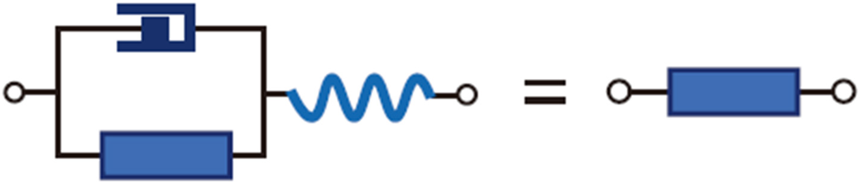
Upon completing the discussion on convergence, we naturally turn to examining the convergence result—that is, the solution for the fractal operator’s value. As the cornerstone of physical fractal theory, this problem now has a well-established and effective solution framework.

This methodology evolved through iterative hypothesis and empirical validation, representing a logically elegant outcome. Its core lies in the equivalence between the fractal unit cell and the holistic fractal element (as illustrated in Figure 6), formalized by the governing Equation (18):

$${\displaystyle \frac{1}{\frac{1}{a}+\frac{1}{b+T}}}=T.$$

(18)

The derivation of Figure 6 stems from the transitivity of equivalence relations; since both the fractal unit cell and the holistic fractal element are individually equivalent to the fractal diagram, it follows that the unit cell must equal the holistic element. By evaluating the two circuit diagrams and leveraging the undetermined nature of the holistic fractal element, we obtain Equation (18) governing the fractal operator. This equation is typically quadratic, and its solution (a square root expression) yields the operator’s value when the positive root is selected.

While this solution is remarkably concise and effective, it has historically lacked a theoretical foundation. However, the revealed continued fraction structure now provides the missing logical basis.

The quadratic nature of the equation and solution is directly explained by Theorem 4, which states that real quadratic irrationals are isomorphic to periodic continued fractions. Since the fractal operator itself is a periodic continued fraction operator, it naturally admits a quadratic radical representation.

The issue of root selection is inherently resolved through the convergence analysis. Notably, the convergence corollary explicitly provides the specific convergent value—by definition of the convergent fixed point, it is straightforward to calculate that this value corresponds precisely to the positive root. Conversely, the negative root, representing a divergent fixed point, is physically inadmissible. The detailed calculation is provided in Appendix A.

Current physical fractal theory lacks universally established criteria for root selection, typically relying on case-by-case empirical justification. The continued fraction framework completely resolves this ambiguity—its mathematically derived results align perfectly with prior empirically chosen roots, demonstrating the power of mathematical formalization in physical processes.

The role of the attractive fixed point extends far beyond merely selecting the correct root—it fundamentally reveals the mathematical foundation underlying the entire methodology. As the definitive value of the fractal operator, the convergent fixed point inherently serves as the solution target of existing methods. Thus, this methodology essentially constitutes a fixed-point computation approach.

From the fixed-point perspective, the rationality of the method becomes clearly apparent. By replacing concrete forms with the formalized generating mapping t(w), Equation (18) transforms into:

$$t(T)=T.$$

(19)

This fundamentally reflects the invariance of the fractal operator T under the mapping t(w), precisely encapsulating the classical fixed-point equation f(x) = x. The methodology for solving the fractal operator thus emerges as an application of fixed-point computation within physical fractal spaces, reaffirming how continued fraction structures unveil the intrinsic nature of physical fractal processes. This represents an intellectual extension of mathematical theory into physics, and we formally designate this approach as the fixed-point method.

The fixed-point equation can be easily derived. Definition 7 is listed as follows:

$$\underset{n\to \infty }{\lim }{\left.t^n(w)\right|}_{w=0}=T.$$

(20)

According to the nature of limits, there are:

$$\underset{n\to \infty }{\lim }{\left.t^{n+1}(w)\right|}_{w=0}=T.$$

(21)

By simultaneously solving and simplifying the two equations, we obtain:

$$t(T)=t\circ \underset{n\to \infty }{\lim }{\left.t^n(w)\right|}_{w=0}=\underset{n\to \infty }{\lim }{\left.t^{n+1}(w)\right|}_{w=0}=\underset{n\to \infty }{\lim }{\left.t^n(w)\right|}_{w=0}=T.$$

(22)

Thus, we have rigorously derived the fixed-point equation. It is worth emphasizing that this process also explains the pivotal significance of Definition 7—it fundamentally demonstrates that the fractal operator emerges as a fixed-point solution.

7. Conclusions

This study reveals the intrinsic connection between fractal operators in physical fractal spaces and continued fractions, providing an algebraic foundation for physical fractal theory. By employing generating mappings as a bridge, we demonstrate that the fractal operator in fractal ladders is a special operator with a periodic continued fraction structure, which is directly determined by the series-parallel rules in the circuit diagram.

Furthermore, we extend the classical self-congruent fractal ladder to a generalized fractal ladder that preserves topological invariance while allowing component heterogeneity. Crucially, we prove that the corresponding fractal operator’s algebraic structure transforms into a general continued fraction.

By leveraging established conclusions about periodic continued fractions, this paper provides a general discussion of two longstanding issues in physical fractal theory: operator convergence and solution methods. We rigorously justify the general convergence of fractal operators, thereby supplying the logical foundation for their assumed existence in prior studies. Furthermore, our fixed-point analysis offers a mathematical explanation for the strict positivity of operator values, finally providing theoretical grounding for conventional solution approaches.

These conclusions have already been applied as default (though not rigorously proven) assumptions in previous works addressing specific physical problems [23,24,25]. Moreover, the logical derivation path of these conclusions follows the conventional reasoning process employed in prior studies.

The profound intrinsic connection between continued fractions and fractal operators significantly strengthens the logical foundation of fractal operator theory. Looking ahead, the theoretical framework established in this study—enabled by the introduction of new algebraic structures—undoubtedly opens fresh perspectives for physical fractal research.

We may now leverage existing continued fraction theory to conduct deeper analyses of fractal operators possessing continued fraction structures. However, it should be noted that all discussions in this work are developed specifically for fractal ladders as a particular class of physical fractals. The algebraic structures of fractal operators corresponding to other topological forms of physical fractals remain to be revealed.

This research has also endowed formal continued fraction structures with concrete physical interpretations, representing a major extension of continued fraction methodology. It provides efficient analytical tools for practical problems involving physical fractals, such as biomechanics and rock mechanics.

We firmly believe that subsequent studies built upon this rigorous mathematical foundation will substantially advance physical fractal theory and demonstrate even greater value in engineering applications.