Analytical Description of Three-Dimensional Fractal Surface Wear Process Based on Multi-Stage Contact Theory

Abstract

Accurately revealing the sliding wear mechanisms of mechanical surfaces is crucial for enhancing the performance of mechanical surfaces. This study reveals the mechanism of stage transitions in three-dimensional surface wear processes from a microscopic contact perspective. Firstly, according to the fractal theory, a mathematical model for the critical area scale controlling debris particle formation is established. Secondly, incorporating the contact area scale, a mathematical expression for the wear coefficient of surfaces, is proposed based on the multi-stage contact theory. Finally, the influences of fractal parameters on critical contact load, wear rate, and wear coefficient are systematically examined. The experimental findings substantiate that the proposed wear model exhibits an explicit deterministic formulation and demonstrates high predictive accuracy for the wear rate.

1. Introduction

The frictional wear of rough mechanical component surfaces in practical engineering applications, particularly adhesive wear, directly results in material removal and changes in dimensional profiles, leading to reduced surface precision and shortened component lifespan [1,2,3,4]. Consequently, accurate elucidation of sliding wear mechanisms on rough surfaces, along with the reliable prediction of wear behavior, is indispensable for enhancing operational efficiency and prolonging the service life of mechanical systems and equipment.

Since the discovery of the laws of sliding friction by pioneers such as Leonardo da Vinci [5], there has been a profound advancement in the comprehension of friction science, particularly over the past century [6]. Nonetheless, it was not until 1953 that the development of quantitative surface wear calculation formulas, exemplified by Archard’s wear equation, became established [7]. Although the Archard wear equation is widely employed for analyzing and calculating the surface wear volume and wear rates, it remains fundamentally an empirical formula. Almost all complex wear conditions are encapsulated in a “wear coefficient” that requires experimental measurement. The Archard wear model is frequently adjusted to develop a modified Archard wear model to accommodate the particular conditions when actual conditions differ from those tested [8]. Notably, the fractal theory has found widespread application in calculating surface wear rate models [9]. In general, there are two approaches for calculating the surface wear rate through fractal theory. The first approach, employing the macroscopic Archard wear theory, calculates surface wear volume through the multiplication of the actual contact area and slip distance [10]. Alternatively, the second methodology computes wear volumes at asperity-level contacts and integrates them to determine the total surface wear volume [11,12].

As nanotechnology rapidly advances, research on surface wear has progressed from a macroscopic to a nanoscale perspective, yielding significant breakthroughs and driving rapid development in surface wear modeling [13,14]. One of the considerable advancements in wear research has recently come from molecular dynamics methods. Initially, Rabinowicz and colleagues [15] discovered and experimentally validated a critical scale during the sliding process of surfaces, where smaller wear debris remains adhered while larger debris detaches. The Molinari team investigated the adhesive wear mechanisms of asperities using molecular dynamics methods inspired by the Rabinowicz criterion in 2016 [16]. Their study demonstrates that abrasive wear occurs when the contact area diameter exceeds a critical threshold. Conversely, asperities experience plastic flattening when the contact area diameter falls below this critical value. Subsequently, the team further investigated the wear mechanisms at the asperity level and introduced a wear model that extends from the physical scale of individual asperities to multiple asperities in 2018 [17]. This model offers new insights into wear coefficients and confirms the feasibility of calculating wear coefficients based solely on physical parameters. The Molinari team’s work garnered widespread attention from other researchers subsequently [18,19,20]. These methods bridge asperity-level wear mechanisms with macroscopic surface wear phenomena, establishing a wear coefficient framework grounded in physical parameters rather than empirical correlations. Building upon these foundations, the present investigation employs the critical area scale method to quantify the proportion of asperities that produce wear debris and uses theoretical methods to derive the surface wear coefficient, thereby alleviating the impact of poor repeatability observed in experimental measurements. In contrast to prior studies, this study delves into the plastic deformation of asperities on fractal surfaces to further analyze how surface contact behavior influences wear. Since the surface contact occurs in multiple contact stages during the actual loading process, the entire wear process of the surface also showed multiple stages.

In the wear processes of macroscopic surfaces and individual asperities at the atomic level, transitions between different wear stages are frequently documented and observed across various materials [21,22]. For instance, Wang et al. [23] systematically examined the wear behavior of Mg-Gd-Y-Zr alloys, identifying a characteristic inflection point in wear rate–load curves that demarcates the transition between mild and severe wear regimes at varying sliding velocities. Cho et al. [24] revealed that alumina materials undergo an abrupt transition from mild to severe wear regimes under sliding conditions. Hsu et al. [25] reviewed models for ceramic surface wear and predicted the wear and transition mechanisms under varying conditions. A wear-considering piecewise fractal theory model was proposed by Ni et al. [26], according to which severe wear was found to occur with increasing load ratio, fractal dimension, and scale coefficient. In summary, the existing literature predominantly relies on experimental data [27] or simulation studies [28] and has not effectively provided a theoretical explanation for the underlying mechanisms of surface wear stage transitions.

In light of the above studies, theoretical methods are employed to elucidate the transitions between wear stages by analyzing the three-dimensional fractal surface contact behavior in this study, aiming to reveal the intrinsic mechanisms of surface wear through the contact and deformation characteristics of asperities. This study provides a rational and effective theoretical explanation for wear stage transitions considering contact characteristics, thereby laying a theoretical foundation for improving surface reliability and quality.

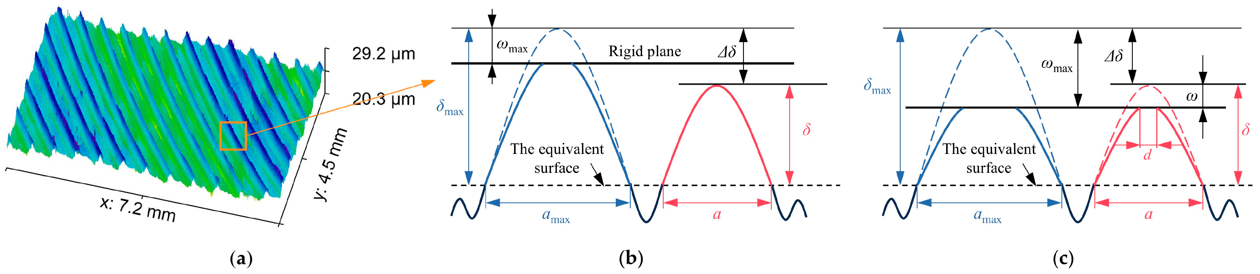
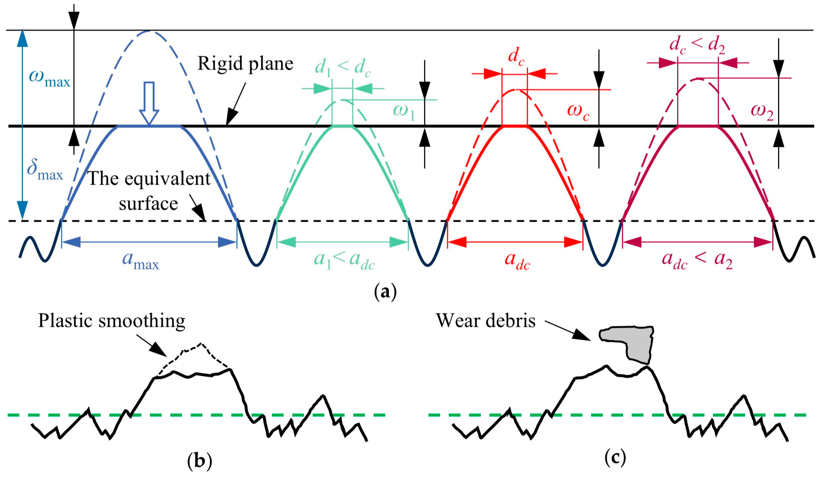
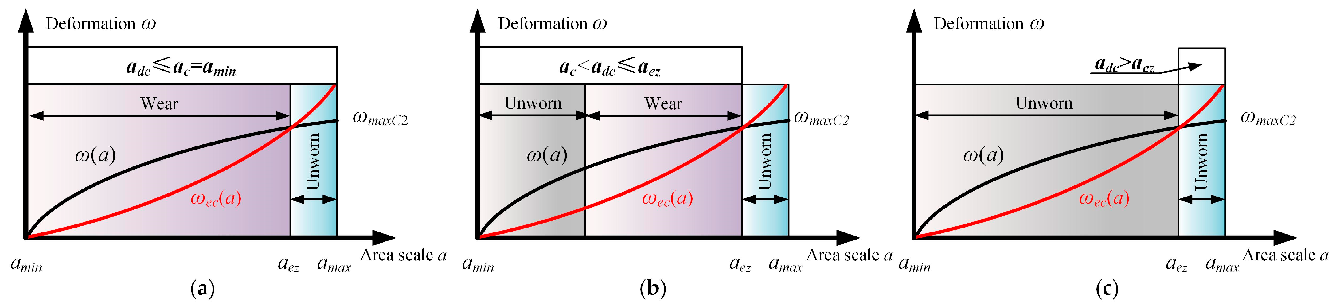
2. Critical Area Scale Model for Controlling the Formation of Abrasive Particles

The microscopic structures of mechanical component surfaces exhibit pronounced self-similar and self-affine characteristics, and the fractal theory is extensively employed to model the mechanical surface. The three-dimensional fractal theory effectively characterizes the multi-scale microscopic morphology of entire surfaces, making it commonly utilized in research [29,30,31]. The three-dimensional fractal function is mathematically formulated as

$$z(x,y)=L{\left(\frac{G}{L}\right)}^{D-2}{\left(\frac{In\gamma }{M}\right)}^{1/2}\sum _{m=1}^M\sum _{n=n_1}^{n_{\max }}{\gamma }^{(D-3)n}\left\{\cos {\phi }_{m,n}-\cos \left[\begin{array}{l}\frac{2\pi {\gamma }^n{(x^2+y{}_2)}^{1/2}}{L}\times \\ \cos ({\tan }^{-1}\left(\frac{y}{x}\right)-\frac{\pi m}{M})+{\phi }_{m,n}\end{array}\right]\right\}$$

(1)

where z(x, y) characterizes the topographical profile; x represents the transverse distance; y defines the longitudinal distance; L signifies the length; D stands for the fractal dimension (2 < D < 3); G corresponds to the fractal roughness; γ refers to the frequency density-related parameter; M indicates the overlap number of the fractal surface wrinkles; φ_m,n denotes the phase; n represents the lowest frequency; n_max is the highest frequency, and its expression is n_max = int(log(L/L_s)/logγ); and L_s signifies the cut-off length.

The height δ of any asperity on the surface is determined by the contact area a through the three-dimensional W-M function, as demonstrated in Figure 1c. Combined with Equation (1), the height δ can be simplified as follows [32,33]

$$\delta =2^{5.5-1.5D}{G}^{D-2}{(\ln \gamma )}^{0.5}{\pi }^{0.5D-1.5}{a}^{1.5-0.5D}$$

(2)

Consequently, the actual deformation of asperities subjected to normal loading can be formulated as

$$\omega ={\omega }_{\mathrm{m}\mathrm{a}\mathrm{x}}-\mathsf{\Delta }\omega ={\omega }_{\max }-2^{5.5-1.5D}{G}^{D-2}{(\ln \gamma )}^{0.5}{\pi }^{0.5D-1.5}(a_{\max }^{1.5-0.5D}-a^{1.5-0.5D})$$

(3)

The parameter ω_max is quantified as the actual deformation of the largest asperity. The expression of the critical contact area at which the asperity begins to contact can be derived from Equation (4).

$$a_c={(a_{\max }^{1.5-0.5D}-{\displaystyle \frac{{\omega }_{\max }}{2^{5.5-1.5D}{G}^{D-2}{(\ln \gamma )}^{0.5}{\pi }^{0.5D-1.5}}})}^{{\displaystyle \frac{1}{1.5-0.5D}}}$$

(4)

The contact area of a single asperity is modeled as a circular section with radius r (diameter d) under fractal theory assumptions. The geometric relationship governing the asperity apex curvature radius R, ω, and r is formulated as

$$R^2={(R-\omega )}^2+r^2$$

(5)

It can be posited that the apex of the asperity can be approximated as a spherical cap. The curvature radius R of the asperity is thereby formulated as

$$R={\displaystyle \frac{2^{1.5D-5.5}{\pi }^{0.5-0.5D}{G}^{2-D}{a}^{0.5D-0.5}}{{(\ln \gamma )}^{0.5}}}$$

(6)

The actual deformation ω typically exhibits negligible magnitude relative to the R, so Equation (6) can be further simplified as

$$R\approx {\displaystyle \frac{r^2}{2\omega }}={\displaystyle \frac{d^2}{8\omega }}$$

(7)

Thus, by integrating Equations (3), (6), and (7), the mathematical relationship between the diameter d and a comprehensively established expressed as follows

$$d=2\sqrt{2\frac{2^{1.5D-5.5}{\pi }^{0.5-0.5D}{G}^{2-D}{a}^{0.5D-0.5}}{{(\ln \gamma )}^{0.5}}\left[\begin{array}{l}{\omega }_{\max }-2^{5.5-1.5D}{G}^{D-2}{(\ln \gamma )}^{0.5}\times \\ {\pi }^{0.5D-1.5}(a_{\max }^{1.5-0.5D}-a^{1.5-0.5D})\end{array}\right]}$$

(8)

Further simplification of Equation (8) can be shown below.

$$d=\sqrt{A_1{a}^{0.5D-0.5}({\omega }_{\max }-B_1+C_1{a}^{1.5-0.5D})}$$

(9)

where A₁, B₁, and C₁ are explicitly defined by Equation (10).

$$\left\{\begin{array}{c}{A}_1=\sqrt{2^{1.5D-2.5}{\pi }^{0.5-0.5D}{G}^{2-D}{(\ln \gamma )}^{-0.5}}\\ B_1=2^{5.5-1.5D}{G}^{D-2}{(\ln \gamma )}^{0.5}{\pi }^{0.5D-1.5}{a}_{\max }^{1.5-0.5D}\\ C_1=2^{5.5-1.5D}{G}^{D-2}{(\ln \gamma )}^{0.5}{\pi }^{0.5D-1.5}\end{array}\right.$$

(10)

Based on the research results of Aghababaei et al. [17], it can be evident that there is a critical length scale d_c that controls the adhesive wear mechanism at the nanoscale. The asperities form wear debris particles when the d exceeds the critical length scale d_c. In contrast, asperities do not produce wear debris particles throughout the plastic smoothing stage. The critical length scale d_c is derived as

$$d_c=\lambda \cdot {\displaystyle \frac{\mathsf{\Delta }w}{({\sigma }_j^2/G_0)}}$$

(11)

when λ = 3 is the shape factor of the three-dimensional contour. The σ_j defines the shear strength of the adhesion, G₀ denotes the shear modulus, and Δw indicates the crack surface energy per unit area [17]. As demonstrated in Figure 2, the asperities undergo wear and produce debris when the a exceeds the critical area scale a_dc. On the contrary, the asperities remain in the plastic smoothing stage. Considering the influence of material properties, Equations (9) and (12) are combined to solve the critical area scale a_dc further.

$$d=2\sqrt{2\frac{2^{1.5D-5.5}{\pi }^{0.5-0.5D}{G}^{2-D}{a}^{0.5D-0.5}}{{(\ln \gamma )}^{0.5}}\left[\begin{array}{l}{\omega }_{\max }-2^{5.5-1.5D}{G}^{D-2}{(\ln \gamma )}^{0.5}\times \\ {\pi }^{0.5D-1.5}(a_{\max }^{1.5-0.5D}-a^{1.5-0.5D})\end{array}\right]}>d_c=\lambda \cdot \frac{\mathsf{\Delta }w}{({\sigma }_j^2/G_0)}$$

(12)

As Equation (12) is a transcendental equation and cannot be solved directly for the critical area scale a_dc, an approximation is obtained using a Taylor series expansion. The specific formula for this approximation is

$$f(a)=A_1{a}^{0.5D-0.5}({\omega }_{\max }-B_1)+C_1{A}_{1}a-{(d_c)}^2$$

(13)

$$f^{\prime }(a)=A_1({\omega }_{\max }-B_1)(0.5D-0.5)a^{0.5D-1.5}+C_1{A}_1$$

(14)

$$f^{″}(a)=A_1({\omega }_{\max }-B_1)(0.5D-0.5)(0.5D-1.5)a^{0.5D-2.5}$$

(15)

When the asperity’s maximum deformation ω_max approaches its maximum height δ_max as defined by Equation (13), it can be obtained as

$$\begin{array}{l}a>\frac{{\lambda }^2\mathsf{\Delta }{w}^2}{{({\sigma }_j^2/G)}^2{A}_1{C}_1}={\lambda }^2\mathsf{\Delta }{w}^2({({\sigma }_j^2/G_0)}^2{2}^{5.5-1.5D}{G}^{D-2}{(\ln \gamma )}^{0.5}{\pi }^{0.5D-1.5}\\ \times \sqrt{2^{1.5D-2.5}{\pi }^{0.5-0.5D}{G}^{2-D}{(\ln \gamma )}^{-0.5}}{)}^{-1}=a_{x0}\end{array}$$

(16)

Combining Equations (13)–(15) and selecting a_x0 as the expansion point for the Taylor series, the approximation can be expressed as

$$\begin{array}{l}f(a)\approx f(a_{x0})+f^{\prime }(a_{x0})(a-a_{x0})+f^{″}(a_{x0}){(a-a_{x0})}^2/2\\ =A_1{a}_{x0}^{0.5D-0.5}({\omega }_{\max }-B_1)+C_1{A}_{1}a-{(d_c)}^2+(A_1({\omega }_{\max }-B_1)(0.5D-0.5)a_{x0}^{0.5D-1.5}+C_1{A}_1)(a-a_{x0})\\ +A_1({\omega }_{\max }-B_1)(0.5D-0.5)(0.5D-1.5)a_{x0}^{0.5D-2.5}=0\end{array}$$

(17)

By further solving Equation (17), the analytical formula of the critical area scale a_dc can be obtained as

$$\begin{array}{l}{a}_{dc}=(a_{x0}(4a_{x0}^{1.5}((A_1(4A_1{C}_1^2{a}_{x0}^3-5A_1{B}_1^2{a}_{x0}^D-5A_1{a}_{x0}^D{\omega }_{\max }^2-A_1{D}^2{a}_{x0}^D{\omega }_{\max }^2+10A_1{B}_1^2{a}_{x0}^D{\omega }_{\max }-\\ 6B_1{a}_{x0}^{D/2+0.5}{d}_c^2+6A_1{B}_1^{2}D{a}_{x0}^D+6a_{x0}^{D/2+0.5}{d}_c^2{\omega }_{\max }+6A_{1}D{a}_{x0}^D{\omega }_{\max }^2-A_1{B}_1^2{D}^2{a}_{x0}^D+2A_1{B}_1{D}^2{a}_{x0}^D{\omega }_{\max }\\ -8D{a}_{x0}^{D/2+0.5}{d}_c^2{\omega }_{\max }-2B_1{D}^2{a}_{x0}^{D/2+0.5}{d}_c^2+10A_1{B}_1{C}_1{a}_{x0}^{D/2+1.5}+2D^2{a}_{x0}^{D/2+0.5}{d}_c^2{\omega }_{\max }-\\ 10A_1{C}_1{a}_{x0}^{D/2+1.5}{\omega }_{\max }-12A_1{B}_{1}D{a}_{x0}^D{\omega }_{\max }+8B_{1}D{a}_{x0}^{D/2+0.5}{d}_c^2-2A_1{C}_1{D}^2{a}_{x0}^{D/2+1.5}{\omega }_{\max }-\\ 12A_1{B}_1{C}_{1}D{a}_{x0}^{D/2+1.5}+12A_1{C}_{1}D{a}_{x0}^{D/2+1.5}{\omega }_{\max }+2A_1{B}_1{C}_1{D}^2{a}_{x0}^{D/2+1.5})))/(4a_{x0}^3){)}^{1/2}+5A_1{B}_1{a}_{x0}^{D/2}-\\ 5A_1{a}_{x0}^{D/2}{\omega }_{\max }+4A_1{C}_1{a}_{x0}^{1.5}-A_1{D}^2{a}_{x0}^{D/2}{\omega }_{\max }-6A_1{B}_{1}D{a}_{x0}^{D/2}+6A_{1}D{a}_{x0}^{D/2}{\omega }_{\max }+A_1{B}_1{D}^2{a}_{x0}^{D/2}))/(3A_1\times \\ B_1{a}_{x0}^{D/2}-3A_1{a}_{x0}^{D/2}{\omega }_{\max }-A_1{D}^2{a}_{x0}^{D/2}{\omega }_{\max }-4A_1{B}_{1}D{a}_{x0}^{D/2}+4A_{1}D{a}_{x0}^{D/2}{\omega }_{\max }+A_1{B}_1{D}^2{a}_{x0}^{D/2}))\end{array}$$

(18)

In summary, the critical area scale a_dc for determining debris generation is established through the scale of asperities. The present investigation derives the formula using the actual deformation ω of three-dimensional surface asperities, specifically concentrating on the normal contact characteristics of the asperities. Furthermore, the critical area scale a_dc incorporates D, G, and material properties, including crack surface energy per unit area, interfacial shear strength, and shear modulus.

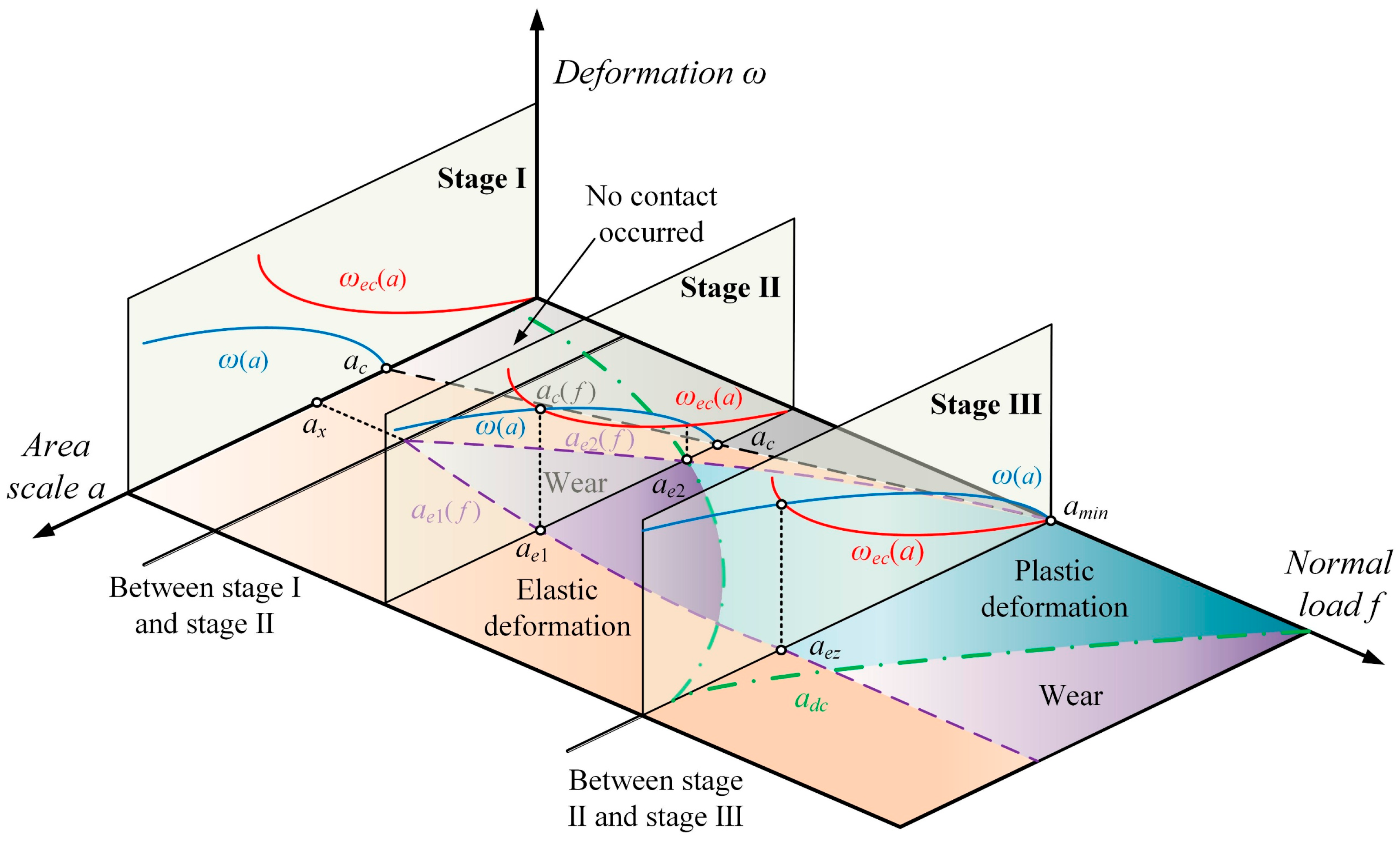
3. Wear Coefficient Modeling of Multiple Asperities Based on Multi-Stage Contact Theory

3.1. A Brief Description of the Wear Coefficient

The wear volume calculated using the Archard model can be expressed as

$$V=k{\displaystyle \frac{NL}{H}}$$

(19)

where V represents the wear volume, k indicates the wear coefficient, N characterizes the normal load, L corresponds to the sliding distance, and H represents the material hardness. By combining Equation (19), the wear volume can be expressed in terms of the actual contact area as depicted below

$$V=kAS$$

(20)

where A represents the actual contact area and S refers to the sliding distance. Equation (20) shows that the wear coefficient k and actual contact area A are the key parameters requiring precise determination in wear volume calculation. The surface wear coefficient model is systematically formulated in this section. The wear coefficient can be typically characterized as the probability of wear debris formation through interactions between contacting asperities on the surfaces [16]. Consequently, it is imperative to accurately distinguish the asperities that produce plastic smoothing and wear debris in the process of analyzing surface wear. A mathematical method is proposed in this study for differentiating fractured and characterizing the surface wear coefficient from a theoretical perspective. This approach employs the critical area scale a_dc to differentiate asperities, with the scale reflecting the necessary conditions for wear debris formation. The wear coefficient can be interpreted as the ratio of asperities that produce wear debris to the total number of asperities on the surface [9]. Consequently, the generation of wear debris from surface asperities necessitates two prerequisites: the asperity must reach the plastic contact stage, while its contact area must exceed a_dc. The wear coefficient of the contact surface can be determined by identifying asperities that meet both the plastic contact stage requirement and the critical area scale condition.

From a microscopic perspective, three-dimensional contact surfaces consist of numerous asperities exhibiting diverse geometrical profiles. The contact area varies between the minimum a_n and the maximum a_m levels during contact. The wear coefficient is mathematically defined as the ratio of asperities experiencing wear to the total asperity population. There must be a lower limit a_LOW and an upper limit a_UP in the mathematical range, within which all asperities undergo wear. Accordingly, the proportion of asperities that generate wear debris on a three-dimensional surface is expressed as

$$k={\displaystyle \frac{{{\displaystyle \int }}_{aLOW}^{aUP}n(a)dl}{{{\displaystyle \int }}_{a_n}^{a_m}n(a)dl}}={\displaystyle \frac{a_{UP}^{0.5-0.5D}-a_{LOW}^{0.5-0.5D}}{a_m^{0.5-0.5D}-a_n^{0.5-0.5D}}}$$

(21)

where n(a) represents the area distribution function of asperity and its functional expression is given by [34]

$$n(a)={\displaystyle \frac{D-1}{2}}{a}_{\max }^{0.5D-0.5}{a}^{-0.5D-0.5}(0<a<a_{\max },2<D<3)$$

(22)

In summary, Equation (21) calculates the proportion of asperities that generate wear debris on a three-dimensional contact surface. Section 3.2 provides a detailed exposition of the modeling process for the wear coefficients of multiple asperities, grounded in the multi-stage contact theory.

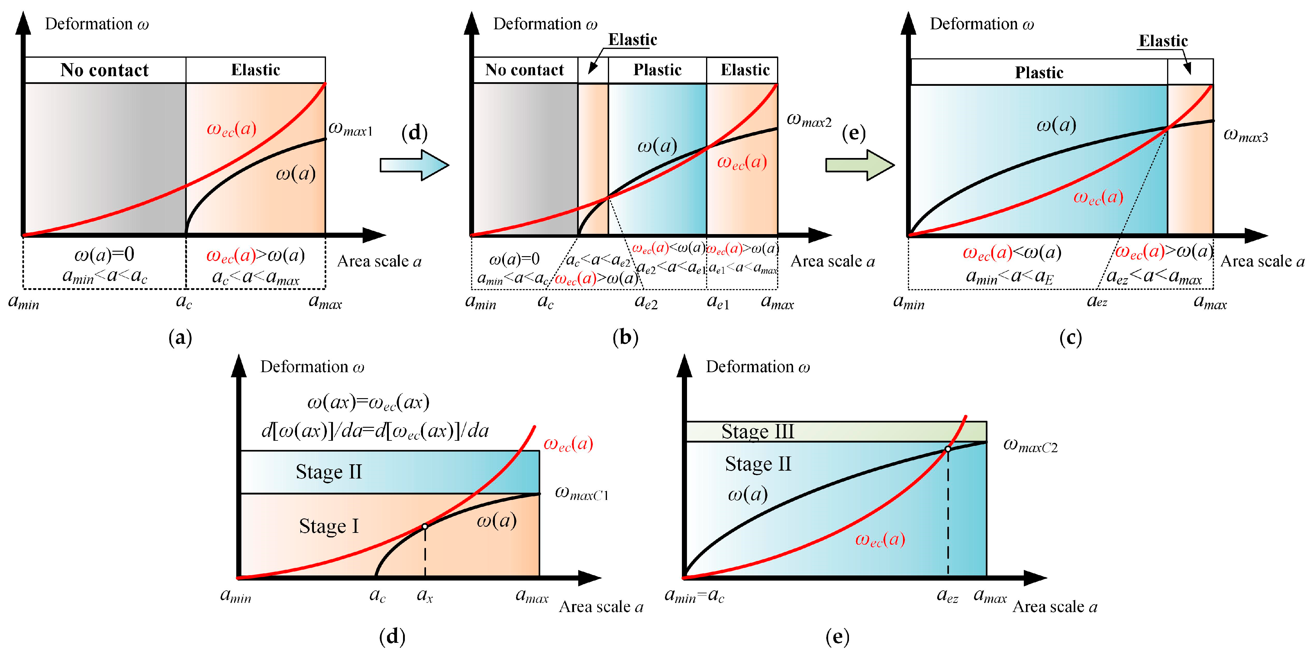
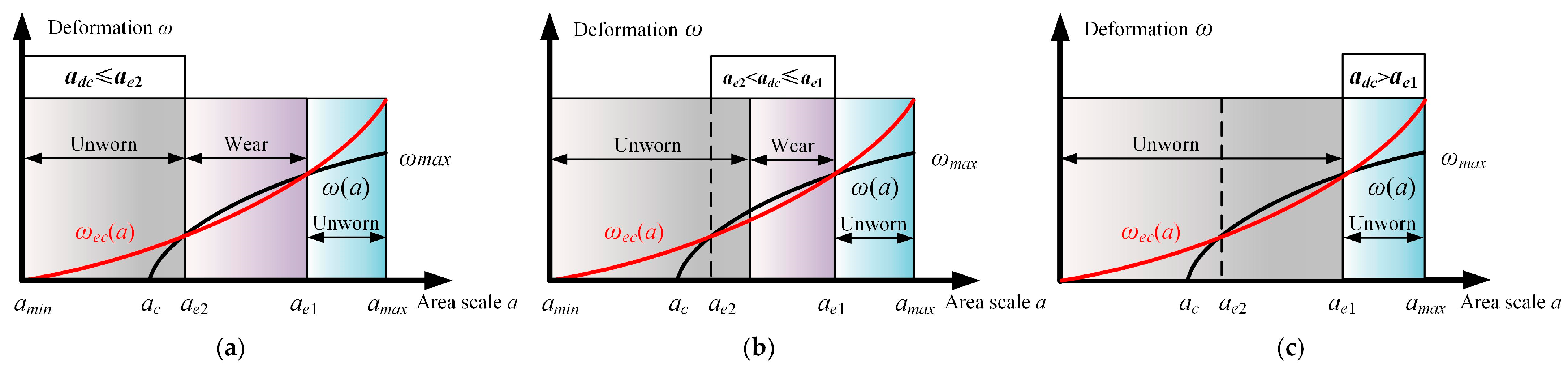
3.2. Wear Coefficient Modeling Based on the Multi-Stage Contact Theory

The wear phase occurs mainly in the plastic contact phase, and the material deformation is irreversible. In the process of adhesive wear on the sliding contact surface, the wear is very small in the lower elastic–plastic deformation range, so the elastic–plastic contact stage is usually ignored in the process of calculating wear [35]. This study consequently disregards wear occurring in the elastic–plastic contact stage, with analytical focus confined to the elastic contact stage and plastic contact stage. According to the literature results [36], the critical deformation at the end of elastic deformation of asperity ω_ec(a) can be acquired as follows [37]

$${\omega }_{ec}(a)={\phi }^2{(2^{1.5}{a}^{0.5}{\pi }^{-0.5})}^{D-1}{G}^{2-D}$$

(23)

where φ represents the coefficient of the interacting materials and takes the value φ = H/(2E).

Increasing normal contact load elevates ω_max, as illustrated in Figure 3, establishing three characteristic contact stages within the contact interface. In stage I, the critical deformation curve ω_ec(a) consistently remains above the actual deformation curve ω(a) of the asperities, indicating that all contacting asperities undergo elastic deformation in this stage.

The curve ω_ec(a) intersects ω(a) in stage II, producing two intersection points, a_e2 and a_e1. The asperities remain in the elastic stage when a_c < a < a_e2. The plastic deformation stage of asperities is maintained for the contact area a within a_e2 < a < a_e1, while the elastic stage persists when a exceeds a_e1. The critical deformation condition ω_maxC1 is established at the tangency point a_x where ω_ec(a) coincides with ω(a).

The fully plastic contact stage occurs in all asperities when the asperity deformation equals the asperity height. The curve ω_ec(a) intersects the curve ω(a) of asperities at a unique contact point a_ez at this point. The asperities undergo the plastic contact stage when the contact area satisfies a_min < a < a_ez, whereas elastic deformation occurs when a exceeds a_ez.

Determining the critical condition ω_maxC1 requires solving the tangent point between ω(a) and ω_ec(a). The equation can be established as the actual deformation coincides with the critical deformation at the tangent point a_x.

$${\phi }^2{(2^{1.5}{a}_x^{0.5}{\pi }^{-0.5})}^{D-1}{G}^{2-D}={\omega }_{\max }-2^{5.5-1.5D}{G}^{D-2}{(\ln \gamma )}^{0.5}{\pi }^{0.5D-1.5}(a_{\max }^{1.5-0.5D}-a_x^{1.5-0.5D})$$

(24)

Simultaneously, since the tangents to ω(a) and ω_ec(a) are the same at the point a_x, differentiating both sides of the equation gives

$$a_x={({\displaystyle \frac{3-D}{D-1}}{\phi }^{-2}{2}^{7-3D}{G}^{2D-4}{(\ln \gamma )}^{0.5}{\pi }^{D-2})}^{{\displaystyle \frac{1}{D-2}}}$$

(25)

The critical deformation condition ω_maxC1 governing the elastic–plastic transition is thus established as

$$\begin{array}{l}{\omega }_{\max C1}=2^{5.5-1.5D}{G}^{D-2}{(\ln \gamma )}^{0.5}{\pi }^{0.5D-1.5}(a_{\max }^{1.5-0.5D}-{(\frac{3-D}{D-1}{\phi }^{-2}{2}^{7-3D}{G}^{2D-4}{(\ln \gamma )}^{0.5}{\pi }^{D-2})}^{\frac{3-D}{2D-4}})+\\ {\phi }^2{2}^{1.5D-1.5}{\pi }^{-0.5D+0.5}{G}^{2-D}{(\frac{3-D}{D-1}{\phi }^{-2}{2}^{7-3D}{G}^{2D-4}{(\ln \gamma )}^{0.5}{\pi }^{D-2})}^{\frac{D-1}{2D-4}}\end{array}$$

(26)

The deformation magnitude of asperities reaches the asperity height during stage II, and the expression of the deformation condition ω_maxC2 can be obtained as

$${\omega }_{\max C2}={\delta }_{\max }=2^{5.5-1.5D}{G}^{D-2}{(\ln \gamma )}^{0.5}{\pi }^{0.5D-1.5}{a}_{\max }^{1.5-0.5D}$$

(27)

Accurately determining the intersection point between ω(a) and ω_ec(a) is crucial for analyzing the multi-stage wear characteristics of the surface throughout the contact phase. The function f(a) can be acquired from Equation (28). The solution of f(a) is the value of the intersection point of ω(a) and ω_ec(a).

$$f(a)={\phi }^2{(2^{1.5}{a}^{0.5}{\pi }^{-0.5})}^{D-1}{G}^{2-D}-{\omega }_{\max }+2^{5.5-1.5D}{G}^{D-2}{(\ln \gamma )}^{0.5}{\pi }^{0.5D-1.5}(a_{\max }^{1.5-0.5D}-a^{1.5-0.5D})$$

(28)

$$f^{\prime }(a)=\frac{(D-1)}{2}{\phi }^2{(2^{1.5}{\pi }^{-0.5})}^{D-1}{G}^{2-D}{a}^{0.5D-1.5}-\frac{3-D}{2}{2}^{5.5-1.5D}{G}^{D-2}{(\ln \gamma )}^{0.5}{\pi }^{0.5D-1.5}{a}^{0.5-0.5D}$$

(29)

$$f^{″}(a)=\frac{(D-1)(D-3)}{4}{\phi }^2{(2^{1.5}{\pi }^{-0.5})}^{D-1}{G}^{2-D}{a}^{0.5D-2.5}-\frac{(3-D)(1-D)}{4}{2}^{5.5-1.5D}{G}^{D-2}{(\ln \gamma )}^{0.5}\times {\pi }^{0.5D-1.5}{a}^{-0.5-0.5D}$$

(30)

As the function f(a) is a transcendental equation and cannot be solved directly, a Taylor series expansion is applied to approximate its solution. Nevertheless, Taylor expansion cannot be applied at x₀ = 0 because f(a) is not differentiable at x₀ = 0. Since Taylor series expansion approximates a complex function locally, errors increase outside this region. Choosing an appropriate expansion point is essential. As a result, the expansion is performed at x₀ = a_ez, where a_ez represents the intersection point of ω_ec(a) and ω(a) in the complete plastic contact stage. The expression for a_ez is given by [38,39]

$$a_{ez}=G{\phi }^{{\displaystyle \frac{1}{2-D}}}{\chi }^{{\displaystyle \frac{1}{4-2D}}}$$

(31)

Substituting Equation (32) yields

$$\begin{array}{l}f(a)=f(a_{ez})+f^{\prime }(a_{ez})(a-a_{ez})+{\displaystyle \frac{f^{″}(a_{ez}){(a-a_{ez})}^2}{2!}}+\mathrm{\dots }+R_n\\ \approx f(a_{ez})+f^{\prime }(a_{ez})(a-a_{ez})+{\displaystyle \frac{f^{″}(a_{ez}){(a-a_{ez})}^2}{2!}}\end{array}$$

(32)

where R_n is the remainder of Taylor’s formula. Thus, the simplification of Equation (32) can be further obtained.

$$\begin{array}{l}{\phi }^2{(2^{1.5}{a}_{ez}^{0.5}{\pi }^{-0.5})}^{D-1}{G}^{2-D}-{\omega }_{\max }+2^{5.5-1.5D}{G}^{D-2}{(\ln \gamma )}^{0.5}{\pi }^{0.5D-1.5}(a_{\max }^{1.5-0.5D}-a_{ez}^{1.5-0.5D})+\\ (\frac{(D-1)}{2}{\phi }^2{(2^{1.5}{\pi }^{-0.5})}^{D-1}{G}^{2-D}{a}_{ez}^{0.5D-1.5}-\frac{3-D}{2}{2}^{5.5-1.5D}{G}^{D-2}{(\ln \gamma )}^{0.5}{\pi }^{0.5D-1.5}{a}_{ez}^{0.5-0.5D})(a-a_{ez})\\ +\frac{{(a-a_{ez})}^2}{2}(\frac{(D-1)(D-3)}{4}{\phi }^2{(2^{1.5}{\pi }^{-0.5})}^{D-1}{G}^{2-D}{a}_{ez}^{0.5D-2.5}-\frac{(3-D)(1-D)}{4}{2}^{5.5-1.5D}{G}^{D-2}{(\ln \gamma )}^{0.5}\times {\pi }^{0.5D-1.5}{a}_{ez}^{-0.5-0.5D})=0\end{array}$$

(33)

The specific expression for a_e1 is shown as Equation (34).

$$a_{e1}={\displaystyle \frac{f_2{a}_{ez}-f_1+\sqrt{{({f_1}^2-f_2{a}_{ez})}^2-2f_2(f-f_1{a}_{ez}+\frac{1}{2}{f}_2{a_{ez}}^2)}}{f_2}}$$

(34)

where f is the value of function f(a) at the a_ez point, f₁ is the first derivative of function f(a) with respect to variable a at the a_ez point, and f₂ denotes the second derivative of function f(a) with respect to a at a_ez. The variable a_e2 denotes the second intersection point between ω(a) and the critical deformation ω_ec(a), located near a_c. Consequently, the Taylor expansion can also be employed to obtain

$$\begin{array}{l}{\phi }^2{(2^{1.5}{a}_c^{0.5}{\pi }^{-0.5})}^{D-1}{G}^{2-D}-{\omega }_{\max }+2^{5.5-1.5D}{G}^{D-2}{(\ln \gamma )}^{0.5}{\pi }^{0.5D-1.5}(a_{\max }^{1.5-0.5D}-a_c^{1.5-0.5D})+\\ (\frac{(D-1)}{2}{\phi }^2{(2^{1.5}{\pi }^{-0.5})}^{D-1}{G}^{2-D}{a}_c^{0.5D-1.5}-\frac{3-D}{2}{2}^{5.5-1.5D}{G}^{D-2}{(\ln \gamma )}^{0.5}{\pi }^{0.5D-1.5}{a}_c^{0.5-0.5D})(a-a_c)\\ +\frac{{(a-a_c)}^2}{2}(\frac{(D-1)(D-3)}{4}{\phi }^2{(2^{1.5}{\pi }^{-0.5})}^{D-1}{G}^{2-D}{a}_c^{0.5D-2.5}-\frac{(3-D)(1-D)}{4}{2}^{5.5-1.5D}{G}^{D-2}{(\ln \gamma )}^{0.5}\times {\pi }^{0.5D-1.5}{a}_c^{-0.5-0.5D})=0\end{array}$$

(35)

Therefore, the specific expression for a_e2 can be given as

$$a_{e2}={\displaystyle \frac{f_2’a_c-f_1’+\sqrt{{(f_1{’}^2-f_2’a_c)}^2-2f_2’(f’-f_1’a_c+\frac{1}{2}{f}_2’{a_c}^2)}}{f_2’}}$$

(36)

where f’ is the value of function f(a) at the a_ez point and f₁’ and f₂’ denote the first and second derivatives of function f(a) with respect to a at a_c, respectively. As each contact stage influences surface wear characteristics, the wear coefficient variations across stages must be examined. No wear occurs during stage I, as all asperities remain in the elastic contact phase, where the two conditions necessary for wear debris formation remain unsatisfied.

Figure 4 illustrates the wear behavior of asperities in stage II. Stage II can be divided into three distinct situations according to the intersections of a_e2 and a_e1. Asperities are classified as the first stage when the critical area scale a_dc satisfies a_dc < a_e2. In this case, the asperities produce wear debris when a_e2 < a < a_e1. The asperities do not experience wear in other regions, as the two conditions necessary for the generation of wear debris are not satisfied. Meanwhile, asperities are classified as the second stage when the critical area scale a_dc satisfies a_e2 < a_dc <a_e1. The wear debris is generated when a_dc < a < a_e1. In other regions, wear does not take place. During the third stage, no wear occurs in the entire contact area when a_dc > a_e1.

The generation of plastic deformation leads to wear in stage II. It is essential to combine the critical area scale a_dc to determine further whether the asperity is in the plastic smoothing stage or the stage of producing wear debris. The wear coefficient for stage II is accordingly derived as

$$k=\left\{\begin{array}{c}0,a_{dc}>a_{e1}\\ (a_{e1}^{0.5-0.5D}-a_{dc}^{0.5-0.5D}){(a_m^{0.5-0.5D}-a_n^{0.5-0.5D})}^{-1},a_{e2}<a_{dc}<a_{e1}\\ (a_{e1}^{0.5-0.5D}-a_{e2}^{0.5-0.5D}){(a_m^{0.5-0.5D}-a_n^{0.5-0.5D})}^{-1},a_{dc}<a_{e2}\end{array}\right.$$

(37)

The asperities in stage III remain in the plastic contact stage when a satisfies a_min < a < a_ez, with this relationship explicitly depicted in Figure 5. The asperities undergo elastic deformation when a exceeds a_ez. As a result, stage III can be categorized into three distinct cases based on a_min and a_ez. The asperities are in the first stage when a_dc ≤ a_min. The asperities undergo wear in the range a_min < a < a_ez, leading to the generation of debris. The asperities transition to stage II when a_min < a_dc < a_ez. As indicated in the figure, the asperities undergo wear within the range a_dc < a < a_ez. The third stage does not satisfy the conditions for wear when a_dc > a_ez. Hence, the wear coefficient for stage III can be expressed by

$$k=\left\{\begin{array}{c}0,a_{dc}>a_{ez}\\ (a_{aE}^{0.5-0.5D}-a_{dc}^{0.5-0.5D}){(a_m^{0.5-0.5D}-a_n^{0.5-0.5D})}^{-1},a_{\min }<a_{dc}<a_{ez}\end{array}\right.$$

(38)

In summary, the critical area scale of each stage is predominantly governed by D and G so as to further obtain the wear coefficient of the three-dimensional surface. Consequently, this theoretical approach enables wear coefficient prediction through the three-dimensional surface morphological characterization, effectively circumventing the experimental uncertainties and stochastic variability inherent in empirical testing methodologies. Additionally, the surface wear coefficient is mainly determined by the critical area scale a_dc. The wear coefficient established in this section is derived from a microscopic contact perspective, and there is no macroscopic wear coefficient expression in the formula.

4. Establishment of Three-Dimensional Surface Wear Mathematical Model

This study primarily determines the critical area scale at the asperity scale, while the wear process of asperities is further influenced by multi-stage contact phenomena, as illustrated in Figure 6. Specifically, wear does not occur when the asperities are in stage I. The wear area of the asperity changes with the multi-stage contact process as the contact load increases in stages II and III. Since the wear coefficients for each contact stage are established in the previous section, determining the wear rate requires calculating the actual contact area. The expressions for the real contact area in stages I to III, formulated through multi-stage contact theory, are explicitly defined in Equations (39)–(41).

$$A_{\mathsf{{\rm I}}}={{\displaystyle \int }}_{a_c}^{a_{\max }}an(a)da={{\displaystyle \int }}_{a_c}^{a_{\max }}{\displaystyle \frac{D-1}{2}}{a}_{\max }^{0.5D-0.5}{a}^{0.5-0.5D}da({\omega }_{\max }<{\omega }_{\max C1})$$

(39)

$$\begin{array}{l}{A}_{\mathrm{II}}={\int }_{a_c}^{a_{e2}}an(a)da+{\int }_{a_{e2}}^{a_{e1}}an(a)da+{\int }_{a_{e1}}^{a_{\max }}an(a)da({\omega }_{\max C1}<{\omega }_{\max }<{\omega }_{\max C2})\\ ={\int }_{a_c}^{a_{e2}}\frac{D-1}{2}{a}_{\max }^{0.5D-0.5}{a}^{0.5-0.5D}da+{\int }_{a_{e2}}^{a_{e1}}\frac{D-1}{2}{a}_{\max }^{0.5D-0.5}{a}^{0.5-0.5D}da+{\int }_{a_{e1}}^{a_{\max }}\frac{D-1}{2}{a}_{\max }^{0.5D-0.5}{a}^{0.5-0.5D}da\end{array}$$

(40)

$$\begin{array}{l}{A}_{\mathrm{III}}={{\displaystyle \int }}_{a_{\min }}^{a_{ez}}an(a)da+{{\displaystyle \int }}_{a_{ez}}^{a_{\max }}an(a)da({\omega }_{\max C2}<{\omega }_{\max })\\ ={{\displaystyle \int }}_{a_{\min }}^{a_{ez}}{\displaystyle \frac{D-1}{2}}{a}_{\max }^{0.5D-0.5}{a}^{0.5-0.5D}da+{{\displaystyle \int }}_{a_{ez}}^{a_{\max }}{\displaystyle \frac{D-1}{2}}{a}_{\max }^{0.5D-0.5}{a}^{0.5-0.5D}da\end{array}$$

(41)

Following the literature [36], the contact load expressions for asperities under elastic and plastic contact conditions are expressed as

$$\left\{\begin{array}{c}{f}_e={\displaystyle \frac{1}{3}}E{\pi }^{0.5D-2}{2}^{7.5-1.5D}{(\ln \gamma )}^{0.5}{G}^{D-2}{a}^{2-0.5D}\\ f_p=Ha\end{array}\right.$$

(42)

Consequently, the contact load expressions across various stages are derived through Equation (42).

$$\begin{array}{l}{F}_{\mathrm{I}}={{\displaystyle \int }}_{a_c}^{a_{\max }}{f}_{e}n(a)da({\omega }_{\max }<{\omega }_{\max C1})\\ ={\displaystyle \frac{D-1}{3}}{a}_{\max }^{0.5D-0.5}E{\pi }^{0.5D-2}{2}^{6.5-1.5D}{(\ln \gamma )}^{0.5}{G}^{D-2}{{\displaystyle \int }}_{a_c}^{a_{\max }}{a}^{1.5-D}da\end{array}$$

(43)

$$\begin{array}{l}{F}_{\mathrm{II}}={\int }_{a_c}^{a_{e2}}{f}_{e}n(a)da+{\int }_{a_{e2}}^{a_{e1}}{f}_{p}n(a)da+{\int }_{a_{e1}}^{a_{\max }}{f}_{e}n(a)da({\omega }_{\max C1}<{\omega }_{\max }<{\omega }_{\max C2})\\ =\frac{D-1}{3}{a}_{\max }^{0.5D-0.5}E{\pi }^{0.5D-2}{2}^{6.5-1.5D}{(\ln \gamma )}^{0.5}{G}^{D-2}({\int }_{a_c}^{a_{e2}}{a}^{1.5-D}da+{\int }_{a_{e1}}^{a_{\max }}{a}^{1.5-D}da)+{\int }_{a_{e2}}^{a_{e1}}\frac{D-1}{2}H{a}_{\max }^{0.5D-0.5}{a}^{-0.5D+0.5}da\end{array}$$

(44)

$$\begin{array}{l}{F}_{\mathrm{III}}={\int }_{a_{\min }}^{a_{ez}}{f}_{p}n(a)da+{\int }_{a_{ez}}^{a_{\max }}{f}_{e}n(a)da({\omega }_{\max C2}<{\omega }_{\max })\\ =\frac{D-1}{3}{a}_{\max }^{0.5D-0.5}E{\pi }^{0.5D-2}{2}^{6.5-1.5D}{(\ln \gamma )}^{0.5}{G}^{D-2}{\int }_{a_{ez}}^{a_{\max }}{a}^{1.5-D}da+\frac{D-1}{2}H{a}_{\max }^{0.5D-0.5}{\int }_{a_{\min }}^{a_{ez}}{a}^{-0.5D+0.5}da\end{array}$$

(45)

The wear volume expression for the three-dimensional fractal surface is derived by integrating Equations (39)–(45).

$$\begin{array}{l}V=kSA=S\frac{a_{UP}^{0.5-0.5D}-a_{LOW}^{0.5-0.5D}}{a_m^{0.5-0.5D}-a_n^{0.5-0.5D}}\times \\ \left\{\begin{array}{c}\left[\begin{array}{l}{\int }_{a_c}^{a_{e2}}\frac{D-1}{2}{a}_{\max }^{0.5D-0.5}{a}^{0.5-0.5D}da+{\int }_{a_{e2}}^{a_{e1}}\frac{D-1}{2}{a}_{\max }^{0.5D-0.5}{a}^{0.5-0.5D}da\\ +{\int }_{a_{e1}}^{a_{\max }}\frac{D-1}{2}{a}_{\max }^{0.5D-0.5}{a}^{0.5-0.5D}da\end{array}\right]({\omega }_{\max C1}<{\omega }_{\max }<{\omega }_{\max C2})\\ \left[{\int }_{a_{\min }}^{a_{ez}}\frac{D-1}{2}{a}_{\max }^{0.5D-0.5}{a}^{0.5-0.5D}da+{\int }_{a_{ez}}^{a_{\max }}\frac{D-1}{2}{a}_{\max }^{0.5D-0.5}{a}^{0.5-0.5D}da\right]({\omega }_{\max C2}<{\omega }_{\max })\end{array}\right.\end{array}$$

(46)

In Equation (46), the material properties and surface roughness can be determined by experimental measurements, while the maximum asperity deformation is governed by the applied normal load. Since the maximum deformation of asperities varies across different contact stages, diverse approaches must be accepted depending on the specific contact stage of the asperities.

$$\left\{\begin{array}{c}{F}^{*}=F/(E{A}_a)\\ A^{*}=A/(A_a)\end{array}\right.$$

(47)

To eliminate dimensional unit effects on the intrinsic model properties, the contact load and contact area are non-dimensionalized in Equation (47), where A_a specifically denotes the nominal contact area of the fractal surface.

5. Results and Discussion

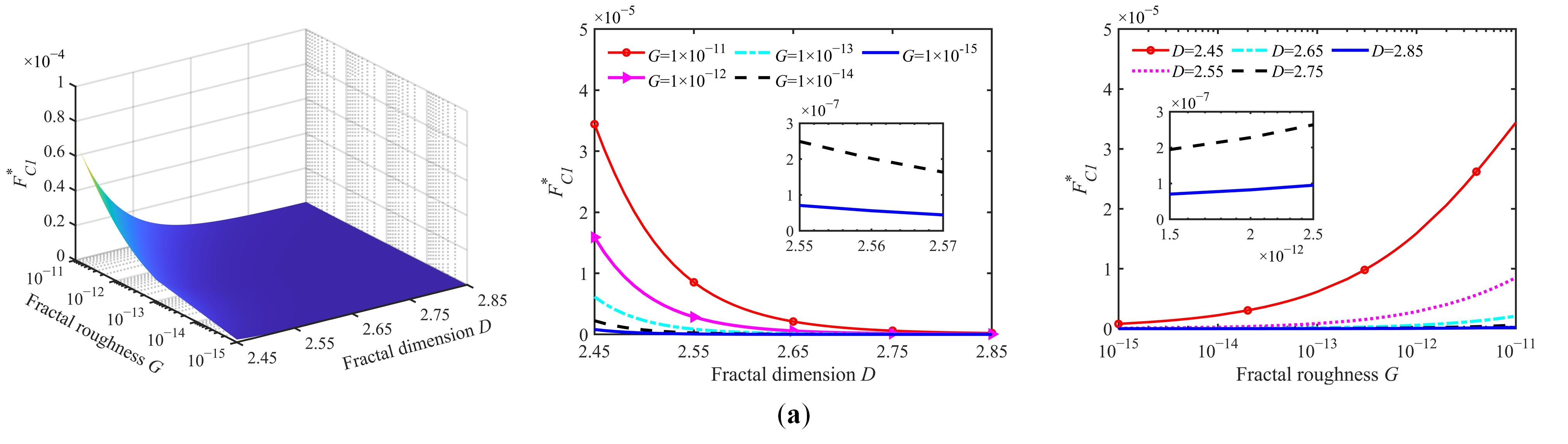
5.1. The Variation of the Critical Load

The critical contact load F_C1* is dictated at the maximum asperity deformation ω_maxC1, representing the threshold load governing the phase transition between stage I and stage II. The elastic deformation exclusively governs when the contact load remains below the critical threshold F_C1*. The critical contact load F_C1* changes as the fractal surface parameters change. The critical contact load is governed not only by surface material properties but also more dominantly by fractal parameters. The critical load F_C2*, calculated using Equation (27), corresponds to the deformation threshold ω_maxC2 in the maximum asperity. The critical contact load F_C2* signifies the onset of full plastic deformation and corresponds to the load threshold at which maximum wear initiates. Figure 7 demonstrates that the dimensionless critical contact loads F_C1* and F_C2* exhibit nearly identical variation trends. From the contact point of view, the variation between the general stiffness and the surface topography is monotonic, and the smoother the surface is, the greater the stiffness is [3]. Variations in surface stiffness govern the evolution of the critical contact load during the stage I-to-stage II transition. Analyzing the critical contact load stage transition can provide some guidance for reducing frictional wear during surface machining.

The critical contact loads F_C1* and F_C2* are obtained with the surface fractal parameters obtained under the conditions of a_max = 1 × 10⁻⁵ m² and a_min = 1 × 10⁻¹⁵ m², as demonstrated in Figure 7a,b. Figure 7a shows the critical contact load F_C1* variation with the surface fractal parameters. For a constant fractal roughness G, the critical contact load F_C1* exhibits a decreasing trend with increasing fractal dimension D. Conversely, F_C1* increases as the fractal roughness G increases for a constant fractal dimension D. Generally, a higher D and a lower G indicate a smoother surface for three-dimensional fractal surfaces. Figure 7a reveals that the critical contact load F_C1* attains its maximum value of approximately 3.5 × 10⁻⁵ under fractal parameter conditions D = 2.5 and G = 1 × 10⁻¹¹ m, representing the maximum transitional load between stage I and stage II contact regimes. Increasing D and decreasing G reduce the critical contact load F_C1*, lowering the load threshold required to transition to stage II.

Figure 7b demonstrates the parametric relationship between the critical contact load F_C2* and surface fractal characteristics. The relationship between surface fractal parameters and F_C2* exhibits nonlinear complexity. The critical contact load F_C2* scales monotonically with the G under fixed D. The critical contact load F_C2* exhibits a convex non-monotonic relationship with D under constant G, initially decreasing before transitioning to an increasing regime. Additionally, F_C2* increases with D under G = 1× 10⁻¹⁵ m, indicating a positive correlation between D and the critical contact load.

Figure 8 compares the two critical contact loads under varying D, G, and maximum contact area a_max from a contact perspective. Figure 8a demonstrates that F_C1* inversely correlates with fractal dimension D, as asperity deformation remains purely elastic in this regime. Due to the smoother surface, the required critical contact load F_C1* is smaller. Conversely, the asperity plastic deformation initiates with rising surface load, inducing an inflection in F_C2* at D = 2.55. The maximum contact area a_max directly governs the number of contacting asperities on fractal surfaces, thereby influencing the critical contact loads F_C1* and F_C2* during wear processes. The dimensionless contact loads F_C1* and F_C2* increase with the maximum contact area a_max, as evidenced in Figure 8c. This is because a larger a_max results in more asperities being in contact, requiring a higher critical contact load.

There is no wear as the pure elastic contact occurs in stage I. The critical area scale a_ez is constant in stage III, so wear remains constant. Accordingly, the wear only varies between the critical contact loads F_C1* and F_C2*. It can be observed that the difference between F_C1* and F_C2* increases with D, G, and a_max from Figure 8. This increase is due to both elastic and plastic contact stages in stage II, resulting in a significant difference between F_C1* and F_C2*.

5.2. The Relationship Between Wear Rate and Normal Contact Load

Practical engineering analyses emphasize the correlation between normal contact load and wear behavior. A linear relationship between the adhesive wear volume and applied normal contact load is established through the Archard wear model. In order to further verify this linear law, the changes in dimensionless contact load and wear rate are plotted as demonstrated in Figure 9 (D = 2.45, G = 1 × 10⁻¹¹ m). The wear rate evolution demonstrates three characteristic phases: negligible wear with the zero volumetric rate in stage I, nonlinear escalation in stage II, and linear progression during stage III.

The surface resides in stage I with zero wear volume under the low dimensionless contact load F*, as evidenced in Figure 9a. The surface wear exhibits nonlinear augmentation with increasing dimensionless contact load F* during stage II. The stage of linearly increasing wear on the surface is in stage III when the dimensionless contact load is further increased. To further analyze these three differing wear stages, the slope change diagram of the curve is constructed, which elucidates the degree of linearity between contact load and wear as the dimensionless contact load increases in Figure 9b. It can be clearly seen from the diagram that the change in the wear stage can be obtained by the change in the slope. The slope is almost zero in stage I. The wear slope increases nonlinearly in stage II, and the maximum slope is 4223.53. The slope remains unchanged at 256.98 in stage III. In essence, the variation in the surface wear coefficient is quantified by the slope. The wear process is divided into three distinct stages due to the influence of surface roughness on the interaction between wear and contact load, with each stage exhibiting diverse wear increment characteristics under varying contact conditions.

Figure 9. The change of surface wear rate and dimensionless contact load F*. (a) The change of wear rate and dimensionless contact load F*. (b) The change of slope and dimensionless contact load F*.

Figure 9. The change of surface wear rate and dimensionless contact load F*. (a) The change of wear rate and dimensionless contact load F*. (b) The change of slope and dimensionless contact load F*.

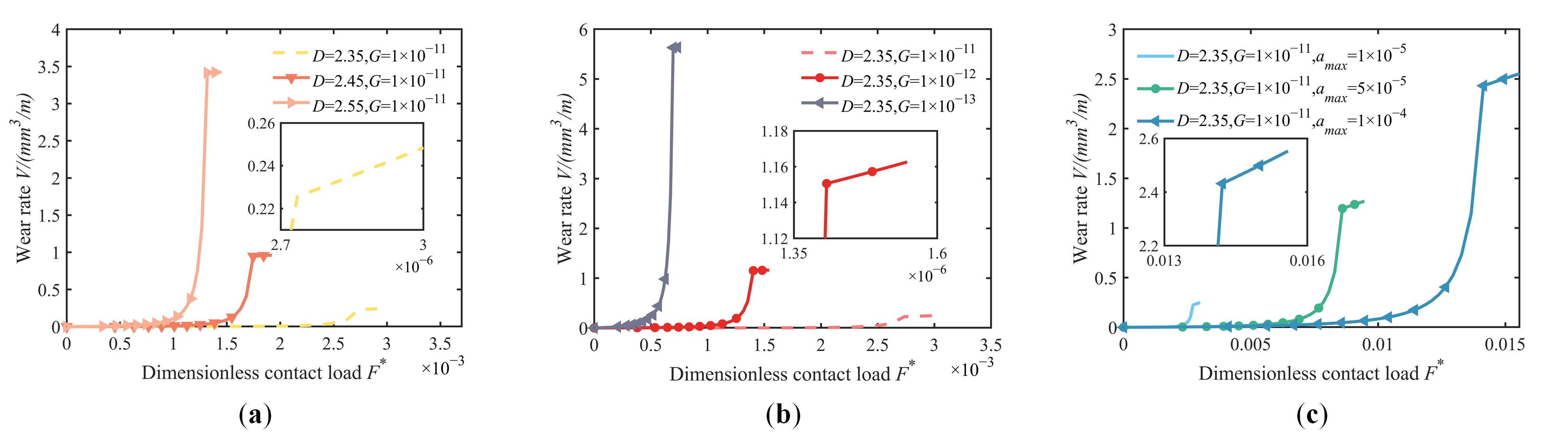
5.3. The Effect of Different Surface Parameters on the Volume Wear Rate

Figure 7 directly demonstrates that rougher fractal surfaces necessitate higher critical contact loads F_C1*. The fractal surface is relatively rough, so the area of wear to zero is longer when D is 2.35 in Figure 10a. The surface becomes smoother as D increases, requiring a smaller critical contact load F_C1*, so the area with wear of zero is shorter. Furthermore, the figure illustrates that alterations in the F*-V curve’s slope reflect the shift between various contact stages. The F*-V curve slope exhibits a pronounced increase with rising fractal dimension D during stage II, indicating a faster intensification of wear rate as contact loads grow.

Figure 10b delineates the correlation between contact load F* and volumetric wear rate V across distinct fractal roughness parameter G conditions. The critical contact load F_C1* is also larger when G is relatively large (G = 1 × 10⁻¹¹ m), and the area where the wear is zero is longer. Additionally, the three curves in the figure all exhibit a concave shape in stage II, consistent with the trend observed in Figure 10a under unlike D conditions. Nevertheless, the influence of fractal roughness parameter G variations on volumetric wear rate V becomes significantly amplified under constant fractal dimension D conditions.

Figure 10c depicts the variation in the volumetric wear rate under different maximum contact areas a_max. The figure demonstrates that the F*-V curve magnitude increases with rising a_max. The number of asperities in contact on the three-dimensional fractal surface rises, leading to a higher volumetric wear rate.

In summary, D, G, and the maximum contact area a_max all exert a direct influence on the volumetric wear rate when the normal contact load and material properties are fixed. Consequently, to achieve effective minimization of surface volumetric wear rates in practical engineering applications, the mechanical surface performance can be improved by increasing D and reducing G and a_max.

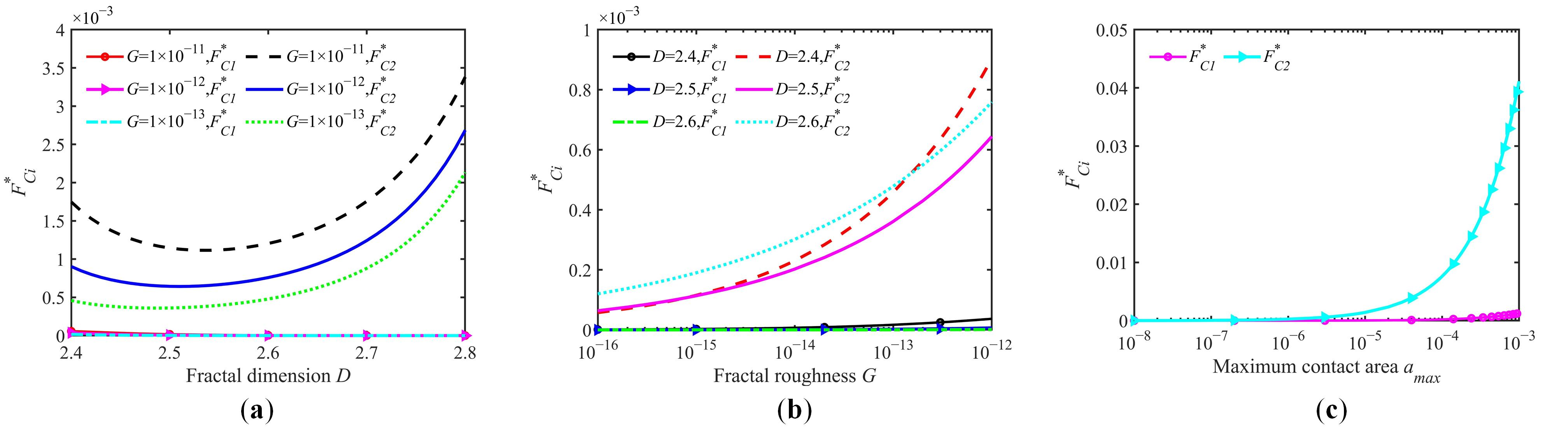
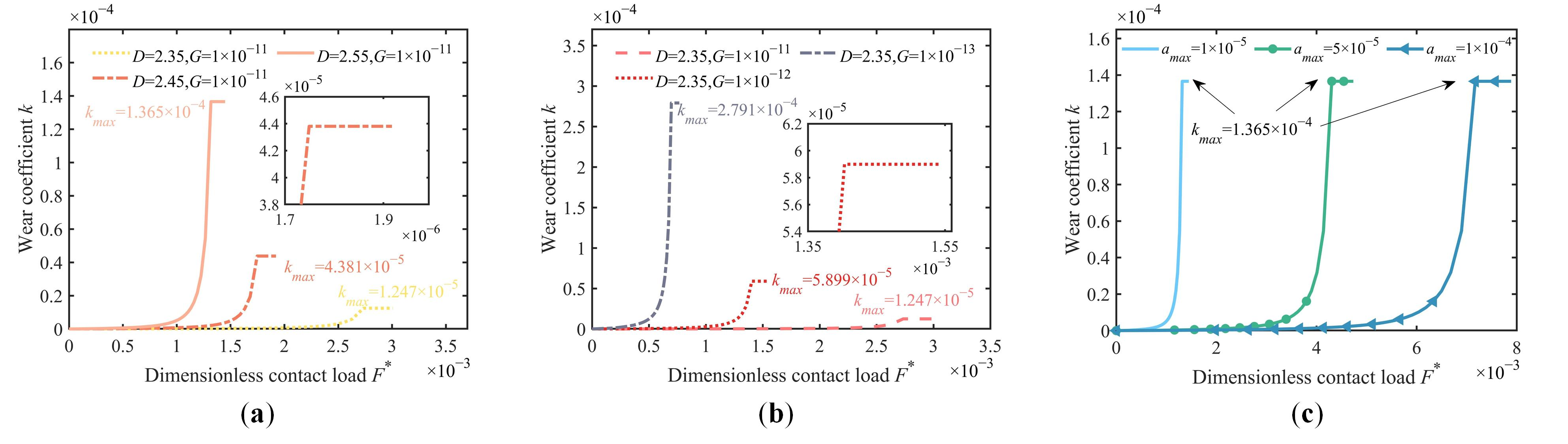
5.4. The Influence of Different Surface Parameters on the Wear Coefficient

The factor determining the wear is the surface fractal parameter when the normal load and material properties are constant. In addition to the volumetric wear rate, various surface parameters also influence the surface wear coefficient. Figure 11a demonstrates that the wear coefficient progressively increases with the contact load across D values of 2.35, 2.45, and 2.55 before reaching a steady value. The elastic deformation only occurs during stage I, resulting in a wear coefficient of zero. The wear coefficient k rises nonlinearly as the contact load increases in stage II, as described by Equation (37). The a_ez does not increase with the contact load in stage III, leading to a constant wear coefficient, according to Equation (38). The maximum wear coefficient measures 1.247 × 10⁻⁵ at D = 2.35, while it attains 1.365 × 10⁻⁴ at D = 2.55, demonstrating that higher fractal dimension D values correspond to elevated maximum wear coefficients.

As illustrated in Figure 11b, variation curves of the wear coefficient under different fractal roughness G conditions are depicted. The figure shows that the maximum wear coefficient increases as G decreases. Specifically, when the fractal roughness G is 1 × 10⁻¹³ m, the maximum wear coefficient is 2.791 × 10⁻⁴. Figure 11c demonstrates the wear coefficient variation under different maximum contact area a_max conditions. Notably, the maximum wear coefficient k_max remains consistent at 1.365 × 10⁻⁴ across the three curves as the a_max increases. This is because a_max essentially reflects the number of contacting asperities and only affects the critical contact load F_C2* required for the transition from stage II to stage III. As a_max increases, F_C2* also increases. Thus, a_max does not influence the variation of the wear coefficient based on Equations (37) and (38).

In addition, the three-dimensional fractal surface wear model established within the current investigation, constructed upon multi-stage contact theory, primarily focuses on the initial wear stage under non-severe deformation conditions. The model’s accuracy may decrease under high-speed and high-load operating conditions, as these operating conditions are excluded from its defined scope.

6. Experimental Verifications

6.1. The Experimental Process

The experimental setup included the Rtec multifunctional friction and wear tester (MFT-5000, San Jose, CA, USA), the Rtec three-dimensional white-light optical interferometer (UP-2000, San Jose, CA, USA), and the Ohaus precision electronic analytical balance (AX124ZH/E, Parsippany, NJ, USA). The disc specimen in the experimental configuration has a radius R₁ = 2.5 cm and thickness H₁ = 0.5 cm, while the cylindrical pin is characterized by a radius R₂ = 3 mm and height H₂ = 8 mm. In order to ensure that the disc does not shift during the wear process, the screw attached to the disc fixture on the friction and wear tester was adjusted to fix the disc in place. Additionally, the built-in level of the force sensor was adjusted to ensure planar contact between the cylindrical pin and disc. The Rtec three-dimensional surface white-light interferometer consisted primarily of a non-contact optical measurement system with a lateral resolution of 0.04 μm. A point-by-point scanning method was used to obtain three-dimensional point cloud data of surfaces with different processing methods during the measurement process. The three-dimensional surface morphology data was then post-processed using the Gwyddion (version 2.52) surface topography evaluation software to obtain a complete 3D surface profile.

The disc specimens were fabricated from Q235 steel supplied by certified manufacturers in Xi’an, Shaanxi Province, China, utilizing identical production-grade lathes, grinding machines, and CNC milling machines to ensure that the surface roughness error of all machined surfaces was within ±5%. The identically processed surfaces underwent careful polishing with sandpaper of the same grit. The error remained within ±2% to ensure the consistent initial surface roughness for the friction pair. The material of the standard cylindrical pin was the 304 stainless steel material. For the purpose of maintaining test accuracy and reliability, all disc specimens and cylindrical pins were manufactured using the standard production process, with hardening treatments omitted from all processed surfaces. The cylindrical pin’s surface demonstrated superior smoothness and increased hardness when compared to surfaces machined through alternative processing methods during testing. The cylindrical pin surface was idealized as rigid, while the surface morphology of the disc specimen can be treated as an equivalent fractal surface. The analysis assumed that wear occurs exclusively on the disc specimen surface. The rationality of this test hypothesis can be confirmed in Reference [36]. All experimental parameters are detailed in Table 1. An Ohaus precision electronic analytical balance with ±0.0002 g linear error and 0.0001 g measurement precision was utilized to measure specimen mass before and after wear.

The relationship between the three-dimensional surface wear rate and the normal load change was systematically analyzed using the control variable method in the experiment. Under constant conditions for other influencing factors, the wear rate variations of the turning, grinding, and milling surfaces were analyzed under diverse normal load conditions. A three-dimensional white-light interferometer was first employed to acquire surface morphology data of distinct specimens. The D and G corresponding to turning, milling, and grinding surfaces were calculated through the structural function method, with computational results comprehensively documented in Table 1. Next, the rotary module was selected in the Rtec tribological test machine software (MFT - Shortcut 22) module, with the rotation radius set to 5 mm. Normal loads were applied in stepped increments spanning 30 N to 150 N at 30 N intervals, while slip distance was defined as 30 rotational cycles. The analysis step duration was set to 3 min. After the wear process was completed, the specimens were removed, cleaned, and dried. Finally, the Ohaus precision electronic analytical balance was employed to measure the mass difference of the specimen. The surface wear volume was determined using the mathematical relationship between mass, volume, and density.

Table 1. Detailed parameters of the specimen during the test.

Factors	Turning Surfaces	Grinding Surfaces	Milling Surfaces	Cylindrical Pins
Material properties	Q235 steel			304 stainless steel
Fractal dimension (D)	2.420	2.347	2.384	-
Fractal roughness (G)	1.032 × 10−11 m	1.210 × 10−11 m	1.532 × 10−11 m	-
Young’s modulus	210 GPa			193 GPa
Hardness	155 HB			200 HB
Poisson ratio	0.27			0.3
Number of specimens	15			50
Radius of the specimen	R1 = 1.25 cm			H1 = 0.3 mm
Height of the specimen	R2 = 0.5 cm			H2 = 8 mm

Table 1. Detailed parameters of the specimen during the test.

Factors	Turning Surfaces	Grinding Surfaces	Milling Surfaces	Cylindrical Pins
Material properties	Q235 steel			304 stainless steel
Fractal dimension (D)	2.420	2.347	2.384	-
Fractal roughness (G)	1.032 × 10−11 m	1.210 × 10−11 m	1.532 × 10−11 m	-
Young’s modulus	210 GPa			193 GPa
Hardness	155 HB			200 HB
Poisson ratio	0.27			0.3
Number of specimens	15			50
Radius of the specimen	R1 = 1.25 cm			H1 = 0.3 mm
Height of the specimen	R2 = 0.5 cm			H2 = 8 mm

Figure 12 depicts the alterations in the three-dimensional morphology and friction coefficient of the turning, grinding, and milling surfaces before and after wear under a normal load of F = 60 N. The averaged friction coefficients measured 0.157 for the turning surface, 0.151 for the grinding surface, and 0.134 for the milling surface. Friction coefficients across machined surfaces exhibited a corresponding increase with elevating normal load magnitudes. This increase arose from the initial wear stage, inducing a progressive friction coefficient elevation with increasing normal load.

6.2. Comparison of Simulation and Test Results

Three wear tests were conducted on surfaces with the same machining method when the normal load remained constant. The experimental results were averaged to reduce the installation error and equipment error during the experiment. Figure 13 presents a comparative analysis between experimental measurements of dimensionless contact load F* and volumetric wear rate V for distinct surface types and the corresponding computational results derived from the proposed model. With the increase in contact load, two distinct wear stages were observed. The wear rate remained minimal under relatively low contact load conditions. Conversely, the wear rate gradually increased with higher contact loads. This wear phenomenon has been previously documented in the academic literature [40]. The model-predicted critical contact force corresponded precisely to the inflection point on the dimensionless contact load and wear rate curve observed in experimental measurements. This alignment represents the “transition” from minor wear to severe wear, further validating the accuracy of the prediction model. Notably, the curve for wear rate versus contact load in stage III did not exhibit a linear increase with increasing contact load. This absence of a linear trend was attributed to the relatively low loads applied in the experiments.

As illustrated in the figure, the change trend of wear rate was consistent with the increase of dimensionless contact load compared with the model in Reference [9]. However, the model proposed in this study demonstrated superior accuracy in predicting wear rates for turning and milling surfaces compared to the model from Reference [9]. Notably, for grinding surfaces, the predictive performance of the present model was slightly inferior to that of Reference [9] during stage I, while its prediction of the wear rate was marginally higher in stage II. Across the three machining surfaces (turning, grinding, and milling), the maximum relative errors between the predicted values of the proposed model and the experimentally measured values were 18.42%, 18.76%, and 23.92%, respectively. Collectively, the model demonstrated acceptable prediction accuracy, with maximum relative errors consistently maintained below 25%. Discrepancies between model predictions and experimental outcomes may stem from factors such as the presence of third-body effects or measurement errors inherent in the experimental process. In conclusion, the surface wear model established based on the multi-stage contact theory in this paper achieved high-precision prediction of the surface wear rate under different processing methods. Furthermore, this study provides an in-depth exploration of the mechanism governing wear stage transitions based on critical area scale variations, thereby offering a theoretical foundation for this phenomenon.

7. Conclusions

Based on multi-stage contact theory, this study introduces a three-dimensional fractal surface wear model that reveals the stage transition mechanisms in the surface wear process from a microscopic contact perspective. The model is established to define the critical region scale of plastic deformation and abrasive particle formation through a systematic analysis of asperity contact behavior. A mathematical expression for the wear coefficient is proposed based on three-dimensional fractal contact theory, demonstrating independence from empirical or experimental data. By integrating the mathematical expression for the wear coefficient with multi-scale contact theory, precise predictions of surface wear rates for various machining methods are achieved. The study further explains wear stage transitions based on critical area scale variations. The conclusions of this study are as follows.

(1)

The volumetric wear rate exhibits nonlinear variation with the contact load under specific operating conditions. It becomes more linear when the contact load is higher, and the transition in wear stages aligns with changes in wear rate stages.

(2)

Surface parameters exhibit distinct impacts on the critical contact load and wear coefficient. Higher surface roughness makes it easier for the surface to enter stage II. Elevated fractal dimension D coupled with reduced fractal roughness G correspond to increased maximum wear coefficient values. In contrast, variations in the maximum asperity contact area a_max demonstrate negligible influence on wear coefficient magnitude.

(3)

The comparison between pin-on-disc wear test results and model predictions reveals that the maximum relative errors for turning, grinding, and milling surfaces are 18.42%, 18.76%, and 23.92% respectively, all confined within 25%. Compared with existing models, the wear rate prediction model developed in this study based on multi-stage contact theory for three-dimensional surfaces demonstrates higher prediction accuracy. These findings simultaneously validate the existence of the three-dimensional surface multi-stage wear phenomenon proposed previously, establishing a theoretical foundation for mechanistically understanding three-dimensional surface multi-stage wear.

(4)

The surface wear model established in this study focuses primarily on the initial wear stage under non-severe deformation conditions. Its accuracy may decrease under high-speed and high-load operating conditions. In addition, this study does not fully consider the influence of complex processes, such as the retention of wear debris, on the actual friction and wear behavior, which can be further discussed in the future.

References

1. Burwell, J.T.; Strang, C.D. On the empirical law of adhesive wear. J. Appl. Phys. 1952, 23, 18–28. [Google Scholar] [CrossRef]
2. Mishra, T.; De Rooij, M.; Schipper, D.J. The effect of asperity geometry on the wear behaviour in sliding of an elliptical asperity. Wear 2021, 470–471, 203615. [Google Scholar] [CrossRef]
3. Shen, F.; Li, Y.H.; Ke, L.L. A novel fractal contact model based on size distribution law. Int. J. Mech. Sci. 2023, 249, 108255. [Google Scholar] [CrossRef]
4. Li, Y.H.; Shen, F.; Güler, M.A.; Ke, L.L. An efficient method for electro-thermo-mechanical coupling effect in electrical contact on rough surfaces. Int. J. Heat Mass Transf. 2024, 226, 125492. [Google Scholar] [CrossRef]
5. Pitenis, A.A.; Dowson, D.; Gregory Sawyer, W. Leonardo da vinci’s friction experiments: An old story acknowledged and repeated. Tribol. Lett. 2014, 56, 509–515. [Google Scholar] [CrossRef]
6. Zhang, H.; Goltsberg, R.; Etsion, I. Modeling adhesive wear in asperity and rough surface contacts: A review. Materials 2022, 15, 6855. [Google Scholar] [CrossRef] [PubMed]
7. Archard, J.F. Contact and rubbing of flat surfaces. J. Appl. Phys. 1953, 24, 981–988. [Google Scholar] [CrossRef]
8. Liu, B.; Bruni, S.; Lewis, R. Numerical calculation of wear in rolling contact based on the archard equation: Effect of contact parameters and consideration of uncertainties. Wear 2022, 490–491, 204188. [Google Scholar] [CrossRef]
9. Yu, X.; Sun, Y.; Liu, M.; Wu, S. Analytical description of the wear process using a multi-stage contact fractal approach. Wear 2024, 548–549, 205364. [Google Scholar] [CrossRef]
10. Shirong, G.; Gouan, C. Fractal prediction models of sliding wear during the running-in process. Wear 1999, 231, 249–255. [Google Scholar] [CrossRef]
11. Zhang, Z.; Ding, X.; Xu, J.; Jiang, H.; Li, N.; Si, J. A study on building and testing fractal model for predicting end face wear of aeroengine’s floating ring seal. Wear 2023, 532–533, 205079. [Google Scholar] [CrossRef]
12. Hao, Q.; Yin, J.; Liu, Y.; Jin, L.; Zhang, S.; Sha, Z. Time-varying wear calculation method for fractal rough surfaces of friction pairs. Coatings 2023, 13, 270. [Google Scholar] [CrossRef]
13. Schirmeisen, A. One atom after the other. Nat. Nanotechnol. 2013, 8, 81–82. [Google Scholar] [CrossRef] [PubMed]
14. Chung, K.H. Wear characteristics of atomic force microscopy tips: A review. Int. J. Precis. Eng. Manuf. 2014, 15, 2219–2230. [Google Scholar] [CrossRef]
15. Rabinowicz, E. The effect of size on the looseness of wear fragments. Wear 1958, 2, 4–8. [Google Scholar] [CrossRef]
16. Aghababaei, R.; Warner, D.H.; Molinari, J.F. Critical length scale controls adhesive wear mechanisms. Nat. Commun. 2016, 7, 11816. [Google Scholar] [CrossRef] [PubMed]
17. Frérot, L.; Aghababaei, R.; Molinari, J.F. A mechanistic understanding of the wear coefficient: From single to multiple asperities contact. J. Mech. Phys. Solids 2018, 114, 172–184. [Google Scholar] [CrossRef]
18. Popov, V.L.; Pohrt, R. Adhesive wear and particle emission: Numerical approach based on asperity-free formulation of rabinowicz criterion. Friction 2018, 6, 260–273. [Google Scholar] [CrossRef]
19. Popov, V.L.; Li, Q.; Lyashenko, I.A. Contact mechanics and friction: Role of adhesion. Friction 2025, 13, 9440964. [Google Scholar] [CrossRef]
20. Dimaki, A.V.; Shilko, E.V.; Dudkin, I.V.; Psakhie, S.G.; Popov, V.L. Role of adhesion stress in controlling transition between plastic, grinding and breakaway regimes of adhesive wear. Sci. Rep. 2020, 10, 1585. [Google Scholar] [CrossRef] [PubMed]
21. Jacobs, T.D.B.; Gotsmann, B.; Lantz, M.A.; Carpick, R.W. On the application of transition state theory to atomic-scale wear. Tribol. Lett. 2010, 39, 257–271. [Google Scholar] [CrossRef]
22. Gotsmann, B.; Lantz, M.A. Atomistic wear in a single asperity sliding contact. Phys. Rev. Lett. 2008, 101, 125501. [Google Scholar] [CrossRef] [PubMed]
23. Wang, Y.B.; Li, L.; An, J. Dry wear behavior and mild-to-severe wear transition in an mg-gd-Y-zr alloy. Surf. Topogr. Metrol. Prop. 2021, 9, 25032. [Google Scholar] [CrossRef]
24. Cho, S.J.; Moon, H.; Hockey, B.J.; Hsu, S.M. The transition from mild to severe wear in alumina during sliding. Acta Metall. Mater. 1992, 40, 185–192. [Google Scholar] [CrossRef]
25. Hsu, S.M.; Shen, M. Wear prediction of ceramics. Wear 2004, 256, 867–878. [Google Scholar] [CrossRef]
26. Ni, X.; Sun, J.; Ma, C.; Zhang, Y. Wear model of a mechanical seal based on piecewise fractal theory. Fractal Fract. 2023, 7, 251. [Google Scholar] [CrossRef]
27. Zhang, J.; Alpas, A.T. Transition between mild and severe wear in aluminium alloys. Acta Mater. 1997, 45, 513–528. [Google Scholar] [CrossRef]
28. Aghababaei, R.; Brink, T.; Molinari, J.F. Asperity-level origins of transition from mild to severe wear. Phys. Rev. Lett. 2018, 120, 186105. [Google Scholar] [CrossRef] [PubMed]
29. Chen, J.; Liu, D.; Wang, C.; Zhang, W.; Zhu, L. A fractal contact model of rough surfaces considering detailed multi-scale effects. Tribol. Int. 2022, 176, 107920. [Google Scholar] [CrossRef]
30. Zhou, W.; Cao, Y.; Zhao, H.; Li, Z.; Feng, P.; Feng, F. Fractal analysis on surface topography of thin films: A review. Fractal Fract. 2022, 6, 135. [Google Scholar] [CrossRef]
31. Zhou, G.; Wang, X.; Feng, F.; Feng, P.; Zhang, M. Calculation of fractal dimension based on artificial neural network and its application for machined surfaces. Fractals 2021, 29, 2150129. [Google Scholar] [CrossRef]
32. Pan, W.; Li, X.; Wang, L.; Mu, J.; Yang, Z. A loading fractal prediction model developed for dry-friction rough joint surfaces considering elastic–plastic contact. Acta Mech. 2018, 229, 2149–2162. [Google Scholar] [CrossRef]
33. Yu, X.; Sun, Y.; Wu, S. Multi-stage contact model between fractal rough surfaces based on multi-scale asperity deformation. Appl. Math. Model. 2022, 109, 229–250. [Google Scholar] [CrossRef]
34. Yan, W.; Komvopoulos, K. Contact analysis of elastic-plastic fractal surfaces. J. Appl. Phys. 1998, 84, 3617–3624. [Google Scholar] [CrossRef]
35. Yin, X.; Komvopoulos, K. An adhesive wear model of fractal surfaces in normal contact. Int. J. Solids Struct. 2010, 47, 912–921. [Google Scholar] [CrossRef]
36. Pan, W.; Sun, Y.; Li, X.; Song, H.; Guo, J. Contact mechanics modeling of fractal surface with complex multi-stage actual loading deformation. Appl. Math. Model. 2024, 128, 58–81. [Google Scholar] [CrossRef]
37. Majumdar, A.; Bhushan, B. Fractal model of elastic-plastic contact between rough surfaces. J. Tribol. 1991, 113, 1–11. [Google Scholar] [CrossRef]
38. Kogut, L.; Etsion, I. Elastic-plastic contact analysis of a sphere and a rigid flat. J. Appl. Mech. 2002, 69, 657–662. [Google Scholar] [CrossRef]
39. Yu, X.; Sun, Y.; Zhao, D.; Wu, S. A revised contact stiffness model of rough curved surfaces based on the length scale. Tribol. Int. 2021, 164, 107206. [Google Scholar] [CrossRef]
40. Brink, T.; Frérot, L.; Molinari, J.F. A parameter-free mechanistic model of the adhesive wear process of rough surfaces in sliding contact. J. Mech. Phys. Solids 2021, 147, 104238. [Google Scholar] [CrossRef]
Figure 1. The contact deformation process of the asperity. (a) Micro-roughness. (b) The asperity deformation case 1 (ωmax  Δδ). (c) The asperity deformation case 1 (ωmax > Δδ).
Fractalfract 09 00463 g001
Figure 2. The influence of critical area scale on adhesive wear. (a) A comparison of the contact area and critical contact area. (b) The plastic smoothing stage. (c) The stage where wear occurs and wear debris is generated.
Fractalfract 09 00463 g002
Figure 3. The multi-stage asperity contact model based on area scale. (a) Stage I; (b) stage II; (c) stage III; (d) the stage I and stage II critical loading deformation of asperity; and (e) the stage II and stage III critical loading deformation of asperity.
Fractalfract 09 00463 g003
Figure 4. The wear characteristics in stage II. (a) The first stage (adcae2). (b) The second stage (ae2 < adcae1). (c) The third stage (ae1 < adc).
Fractalfract 09 00463 g004
Figure 5. The wear characteristics in stage III. (a) The first stage (adcac). (b) The second stage (ac < adcaez). (c) The third stage (aez < adc).
Fractalfract 09 00463 g005
Figure 6. The asperity wear process based on multi-stage contact theory.
Fractalfract 09 00463 g006
Figure 7. The dimensionless critical contact load. (a) Dimensionless critical load FC1*. (b) Dimensionless critical load FC2*.
Fractalfract 09 00463 g007aFractalfract 09 00463 g007b
Figure 8. Comparison of dimensionless critical contact loads under diverse conditions. (a) Comparison of dimensionless contact loads under distinct D conditions. (b) Comparison of dimensionless contact loads under various G conditions. (c) Comparison of dimensionless contact load under different maximum contact area conditions.
Fractalfract 09 00463 g008
Figure 10. The effect of different surface parameters on the volume wear rate. (a) The change in the volume wear rate under various D conditions. (b) The change in the volume wear rate under distinct G conditions. (c) The change in the volume wear rate under diverse amax conditions.
Fractalfract 09 00463 g010
Figure 11. The influence of diverse surface parameters on the wear coefficient. (a) The change in the wear coefficient under different D conditions. (b) The change in the wear coefficient under distinct G conditions. (c) The change in the wear coefficient under unlike amax conditions.
Fractalfract 09 00463 g011
Figure 12. Different surface morphology parameters before and after wear. (ac) The initial surfaces. (df) The original three-dimensional shape data. (gi) The three-dimensional surface wear profile. (jl) The surface friction coefficient under various load conditions.
Fractalfract 09 00463 g012
Figure 13. The surface wear results of various processing methods are compared with the model. (a) The turning surfaces. (b) The grinding surfaces. (c) The milling surfaces. † reference [9]
Fractalfract 09 00463 g013
Disclaimer/Publisher’s Note: The statements, opinions and data contained in all publications are solely those of the individual author(s) and contributor(s) and not of MDPI and/or the editor(s). MDPI and/or the editor(s) disclaim responsibility for any injury to people or property resulting from any ideas, methods, instructions or products referred to in the content.