Mathematical and Physical Analysis of the Fractional Dynamical Model

Abstract

This paper consists of various kinds of wave solitons to the mathematical model known as the truncated M-fractional FitzHugh–Nagumo model. This model explains the transmission of the electromechanical pulses in nerves. Through the application of the modified extended tanh function technique and the modified $(G^{\prime }/G^2)$-expansion technique, we are able to achieve the series of exact solitons. The results differ from the current solutions because of the fractional derivative. These solutions could be helpful in the telecommunication and bioscience domains. Contour plots, in two and three dimensions, are used to describe the results. Stability analysis is used to check the stability of the obtained solutions. Moreover, the stationary solutions of the focusing equation are studied through modulation instability. Future research on the focused model in question will benefit from the findings. The techniques used are simple and effective.

1. Introduction

Equations involving fractional derivatives or integrals are known as fractional differential equations (FDEs). They are utilized to model complex phenomena in various fields, such as physics, engineering, etc. Various kinds of FDEs have been developed, such as the fractional paraxial nonlinear Schrödinger equation [1], the fractional Westervelt model [2], the fractional generalized Pochhammer–Chree equation [3], the fractional Riemann wave solution [4], the fractional density-dependent diffusion reaction model [5], etc. One crucial aspect of the nonlinear physical phenomenon is determining the exact wave solutions of nonlinear fractional differential equations (FDEs). It is true that exact wave solitons offer a wealth of physical data and aid in comprehending the mechanisms underlying a number of physical models, including solid-state physics, chemical physics, biology, plasma physics, optical fibers, and so forth. Many effective techniques for determining the exact wave solutions have emerged in recent years.

In our research, we used the effective and useful techniques, the modified extended tanh function technique and modified $(G^{\prime }/G^2)$-expansion technique. The concerned techniques are utilized for various equations. For instance, the modified extended tanh function technique is utilized for the nonlinear coupled plasma equations [6], the Bogoyavlenskii equation [7], the modified Volterra’s equations [8], the concatenation equation [9], the Biswas–Milovic equation [10], etc. The modified $(G^{\prime }/G^2)$-expansion scheme is utilized for the coupled nonlinear Higgs equations [11], Wazwaz Kaur Boussinesq equation [12], (1+1)-dimensional classical Boussinesq model [13], etc.

Our concerned model is the FitzHugh–Nagumo equation, is given as [14].

$$h_t-h_{xx}-h(1-h)(h-\theta )=0.$$

(1)

Here, $h=h(x,t)$ represents the wave function, and $\theta$ is a parameter. Equation (1) is used to explain the transmission of the electromechanical pulses in nerves. The concerned model is also used in the fields of electromechanics and biology. In the literature, distinct methods are used to solve Equation (1), including the extended tanh–coth function method [14], the Exp-function method [15], the auto-Bäcklund transformation method [16], the improved Riccati expansion method [17], etc.

There are different sections in this paper. Descriptions of the modified extended tanh function scheme and modified $(G^{\prime }/G^2)$-expansion scheme are given in Section 2; the mathematical analysis and exact wave solutions are mentioned in Section 3; graphical representation is mentioned in Section 4; modulation instability (MI) analysis is provided in Section 5; and the conclusion is provided in Section 6.

Truncated M-Fractional Derivative (TMFD)

Definition 1.

Consider $w\left(y\right):[0,\infty )\to \Re$, so TMFD of w of order ϵ is given as [18]:

$$\begin{array}{c}\hfill D_{M,y}^{ϵ,\varrho }w\left(y\right)=\underset{ϵ\to 0}{lim}{\displaystyle \frac{w\left(y{E}_{\varrho }\left(ϵy^{1-ϵ}\right)\right)-w\left(y\right)}{ϵ}},ϵ\in (0,1],\varrho >0,\end{array}$$

where $E_{\varrho }(.)$ shows a TML profile that is given as [19]:

$$\begin{array}{c}\hfill E_{\varrho }\left(z\right)=\sum _{j=0}^i{\displaystyle \frac{z^j}{\Gamma (1+\varrho j)}},\varrho \mathit{is}\mathit{positive}\mathit{and}z\in \mathit{C}.\end{array}$$

Theorem 1.

Suppose a,b are real numbers, and $g,f$ are both differentiable ϵ times for $y>0$, from [18]:

$$\begin{array}{c}\hfill \left(a\right)D_{M,y}^{ϵ,\varrho }(ag\left(y\right)+bf\left(y\right))=a{D}_{M,y}^{ϵ,\varrho }g\left(y\right)+b{D}_{M,y}^{ϵ,\varrho }f\left(y\right).\end{array}$$

$$\begin{array}{c}\hfill \left(b\right)D_{M,y}^{ϵ,\varrho }(g\left(y\right).f\left(y\right))=g\left(y\right)D_{M,y}^{ϵ,\varrho }f\left(y\right)+f\left(y\right)D_{M,y}^{ϵ,\varrho }g\left(y\right).\end{array}$$

$$\begin{array}{c}\hfill \left(c\right)D_{M,y}^{ϵ,\varrho }({\displaystyle \frac{g\left(y\right)}{f\left(y\right)}})={\displaystyle \frac{f\left(y\right)D_{M,y}^{ϵ,\varrho }g\left(y\right)-g\left(y\right)D_{M,y}^{ϵ,\varrho }f\left(y\right)}{{\left(f\left(y\right)\right)}^2}}.\end{array}$$

$$\begin{array}{c}\hfill \left(d\right)D_{M,y}^{ϵ,\varrho }\left(C\right)=0,\mathit{where}C\mathit{is}a\mathit{constant}.\end{array}$$

$$\begin{array}{c}\hfill \left(e\right)D_{M,y}^{ϵ,\varrho }g\left(y\right)={\displaystyle \frac{y^{1-ϵ}}{\Gamma (\varrho +1)}}{\displaystyle \frac{dg\left(y\right)}{dy}}.\end{array}$$

This definition of the fractional derivative fulfills the characteristics of both fractional derivatives as well as the integer order derivative. Fractional differential equations represent the phenomenon in a more prominent form. This fractional derivative provides the solutions closer to the numerical solutions of the concerned equation.

2. Methodologies

2.1. Explanation of Modified Extended $\mathit{tanh}$ Function Technique

In this subsection, we mention the basic steps of the technique. Assuming a fractional nonlinear partial differential equation (NLPDE):

$$\chi (v,v^2,\dots ,{\displaystyle \frac{{\partial }^{ϵ}v}{\partial t^{ϵ}}},{\displaystyle \frac{{\partial }^{2ϵ}v}{\partial t^{2ϵ}}},\dots ,{\displaystyle \frac{\partial v}{\partial x}},{\displaystyle \frac{{\partial }^{2}v}{\partial x^2}},\dots )=0.$$

(2)

Here $v=v(x,t)$ is a wave function. Assuming the following wave transformation:

$$v(x,t)=V\left(\delta \right),\delta =x-\mu {\displaystyle \frac{\Gamma (1+\varrho )}{ϵ}}{t}^{ϵ}.$$

(3)

where $\Gamma$ is a function, $ϵ$ is a parameter, $\delta$ is a variable, x and t are the dimensions, and $\mu$ denotes the soliton velocity. Putting Equation (3) into Equation (2), we obtain a nonlinear ordinary differential equation:

$$\chi (V,V^2,\mu V^{\prime },{\mu }^2{V}^{″},\dots )=0.$$

(4)

Assuming the root of Equation (4) given below:

$$V\left(\delta \right)={\alpha }_0+\sum _{i=1}^m{\alpha }_i{\psi }^i\left(\delta \right)+\sum _{i=1}^m{\beta }_i{\psi }^{-i}\left(\delta \right).$$

(5)

Here ${\alpha }_0,{\alpha }_i,{\beta }_i,(i=1,2,3,\dots ,m)$ are undetermined.

By applying the homogeneous balance method to Equation (4), we obtain a value of m, where $\psi \left(\zeta \right)$ fulfills the following equation:

$${\psi }^{\prime }\left(\delta \right)=\Omega +{\psi }^2\left(\delta \right).$$

(6)

Here, $\Omega$ is a constant, and solutions of Equation (6) are mentioned as [20]:

Case 1: when $\Omega <0$:

$$\psi \left(\delta \right)=-\sqrt{-\Omega }tanh\left(\sqrt{-\Omega }\delta \right),$$

(7)

or

$$\psi \left(\delta \right)=-\sqrt{-\Omega }coth\left(\sqrt{-\Omega }\delta \right).$$

(8)

Case 2: when $\Omega >0$:

$$\psi \left(\delta \right)=\sqrt{\Omega }tan\left(\sqrt{\Omega }\delta \right),$$

(9)

or

$$\psi \left(\delta \right)=-\sqrt{\Omega }cot\left(\sqrt{\Omega }\delta \right).$$

(10)

Case 3: when $\Omega =0$:

$$\psi \left(\delta \right)={\displaystyle \frac{-1}{\delta }}.$$

(11)

Put Equation (5) into Equation (4) with Equation (6). By collecting the coefficient of $\psi \left(\delta \right)$ for each order and putting each order equal to 0, we achieve sets of algebraic equations having ${\alpha }_0,{\alpha }_i,{\beta }_i(i=1,2,3\dots ,m)$, and $\Omega$ with the use of Mathematica software. By solving the sets, we obtain the solutions of Equation (2).

2.2. Explanation of Modified $(G^{\prime }/G^2)$—Expansion Technique

Now, the main steps of this technique are explained as [21].

Step 1:

Consider the Equations (2)–(4).

Step 2:

Consider the root of Equation (4) represented as;

$$Q\left(\delta \right)=\sum _{i=0}^m{\alpha }_i{({\displaystyle \frac{G^{\prime }}{G^2}})}^i,$$

(12)

where ${\alpha }_i(i=0,1,2,3,\dots ,m)$ are to be found where ${\alpha }_j\ne 0$. A new function G = $G\left(\delta \right)$ fulfills the equation,

$${({\displaystyle \frac{G^{\prime }}{G^2}})}^{\prime }={\lambda }_0+{\lambda }_1{({\displaystyle \frac{G^{\prime }}{G^2}})}^2,$$

(13)

where ${\lambda }_0$ and ${\lambda }_1$ denote the constants. We achieve the following solutions to Equation (13) depending on ${\lambda }_0$:

Case 1:${\lambda }_0{\lambda }_1<0$, which yields

$$({\displaystyle \frac{G^{\prime }}{G^2}})=-{\displaystyle \frac{\sqrt{|{\lambda }_0{\lambda }_1|}}{{\lambda }_1}}+{\displaystyle \frac{\sqrt{|{\lambda }_0{\lambda }_1|}}{2}}({\displaystyle \frac{C_{1}sinh\left(\sqrt{{\lambda }_0{\lambda }_1}\delta \right)+C_{2}cosh\left(\sqrt{{\lambda }_0{\lambda }_1}\delta \right)}{C_{1}cosh\left(\sqrt{{\lambda }_0{\lambda }_1}\delta \right)+C_{2}sinh\left(\sqrt{{\lambda }_0{\lambda }_1}\delta \right)}}),$$

(14)

Case 2: if ${\lambda }_0{\lambda }_1>0$, then

$$({\displaystyle \frac{G^{\prime }}{G^2}})=\sqrt{{\displaystyle \frac{{\lambda }_0}{{\lambda }_1}}}({\displaystyle \frac{C_{1}cos\left(\sqrt{{\lambda }_0{\lambda }_1}\delta \right)+C_{2}sin\left(\sqrt{{\lambda }_0{\lambda }_1}\delta \right)}{C_{1}sin\left(\sqrt{{\lambda }_0{\lambda }_1}\delta \right)-C_{2}sin\left(\sqrt{{\lambda }_0{\lambda }_1}\delta \right)}}),$$

(15)

Case 3: if ${\lambda }_0=0$ and ${\lambda }_1\ne 0$, then

$$({\displaystyle \frac{G^{\prime }}{G^2}})=-{\displaystyle \frac{C_1}{{\lambda }_1(C_1\delta +C_2)}}.$$

(16)

Here $C_1$ and $C_2$ are constants.

Step 3:

Put Equation (12) in Equation (4) along with Equation (13), and collect the coefficients of every power of ${\left({\displaystyle \frac{G^{\prime }}{G^2}}\right)}^i$ equal to 0, now manipulate the achieved set having ${\alpha }_i,{\lambda }_0,{\lambda }_1$, $\mu$.

Step 4: Equation (12) of that ${\alpha }_i,\mu$ are obtained in step 3 in Equation (12), and one can gain the results of Equation (2).

3. Mathematical Analysis

Rewrite Equation (1) in the sense of a truncated M-fractional derivative (TMFD) as;

$$D_{M,t}^{ϵ,\varrho }h-D_{M,x}^{2ϵ,\varrho }h-h(1-h)(h-\theta )=0.$$

(17)

applying the given transformation

$$h(x,t)=H\left(\delta \right),\delta =\Gamma (\varrho +1)(\mu {\displaystyle \frac{x^{ϵ}}{ϵ}}-\lambda {\displaystyle \frac{t^{ϵ}}{ϵ}}),$$

(18)

$$D_{M,t}^{ϵ,\varrho }h=-\lambda H^{\prime }.$$

(19)

$$D_{M,x}^{2ϵ,\varrho }h={\mu }^2{H}^{″}.$$

(20)

By using Equations (18) in Equation (17), we obtain the following ODE;

$${\mu }^2{H}^{″}+\lambda H^{\prime }+H(1-H)(H-\theta )=0.$$

(21)

By applying the homogeneous balance method, we obtain $m=1$.

3.1. Exact Solitons Through mEThF Technique

Equation (5) reduces into following form for m = 1.

$$V\left(\delta \right)={\alpha }_1\varphi \left(\delta \right)+{\alpha }_0+{\displaystyle \frac{{\beta }_1}{\varphi \left(\delta \right)}}.$$

(22)

Inserting Equation (22) with Equation (6) in Equation (21), and solving the system, we obtain the following sets:

• Set 1:

$$\left\{{\alpha }_0=1-\mu \sqrt{-2\Omega },{\alpha }_1=-\sqrt{2}\mu ,{\beta }_1=0,\lambda =\mu \left(2\mu \sqrt{-\Omega }-\sqrt{2}\right),\theta =1-2\mu \sqrt{-2\Omega }\right\}.$$

(23)

Case 1:

$$h(x,t)=1-\mu \sqrt{-2\Omega }-\sqrt{2}\mu (-\sqrt{-\Omega }tanh(\sqrt{-\Omega }\Gamma (\varrho +1)(\mu {\displaystyle \frac{x^{ϵ}}{ϵ}}-\lambda {\displaystyle \frac{t^{ϵ}}{ϵ}}))),$$

(24)

or

$$h(x,t)=1-\mu \sqrt{-2\Omega }-\sqrt{2}\mu (-\sqrt{-\Omega }coth(\sqrt{-\Omega }\Gamma (\varrho +1)(\mu {\displaystyle \frac{x^{ϵ}}{ϵ}}-\lambda {\displaystyle \frac{t^{ϵ}}{ϵ}}))).$$

(25)

Case 2:

$$h(x,t)=1-\mu \sqrt{-2\Omega }-\sqrt{2}\mu (\sqrt{\Omega }tan(\sqrt{\Omega }\Gamma (\varrho +1)(\mu {\displaystyle \frac{x^{ϵ}}{ϵ}}-\lambda {\displaystyle \frac{t^{ϵ}}{ϵ}}))),$$

(26)

or

$$h(x,t)=1-\mu \sqrt{-2\Omega }-\sqrt{2}\mu (-\sqrt{\Omega }cot(\sqrt{\Omega }\Gamma (\varrho +1)(\mu {\displaystyle \frac{x^{ϵ}}{ϵ}}-\lambda {\displaystyle \frac{t^{ϵ}}{ϵ}}))).$$

(27)

Set 2:

$$\left\{{\alpha }_0=1-\mu \sqrt{-2\Omega },{\alpha }_1=\sqrt{2}\mu ,{\beta }_1=0,\lambda =\mu \left(\sqrt{2}-2\mu \sqrt{-\Omega }\right),\theta =1-2\mu \sqrt{-2\Omega }\right\}.$$

(28)

Case 1:

$$h(x,t)=1-\mu \sqrt{-2\Omega }+\sqrt{2}\mu (-\sqrt{-\Omega }tanh(\sqrt{-\Omega }\Gamma (\varrho +1)(\mu {\displaystyle \frac{x^{ϵ}}{ϵ}}-\lambda {\displaystyle \frac{t^{ϵ}}{ϵ}}))),$$

(29)

or

$$h(x,t)=1-\mu \sqrt{-2\Omega }+\sqrt{2}\mu (-\sqrt{-\Omega }coth(\sqrt{-\Omega }\Gamma (\varrho +1)(\mu {\displaystyle \frac{x^{ϵ}}{ϵ}}-\lambda {\displaystyle \frac{t^{ϵ}}{ϵ}}))).$$

(30)

Case 2:

$$h(x,t)=1-\mu \sqrt{-2\Omega }+\sqrt{2}\mu (\sqrt{\Omega }tan(\sqrt{\Omega }\Gamma (\varrho +1)(\mu {\displaystyle \frac{x^{ϵ}}{ϵ}}-\lambda {\displaystyle \frac{t^{ϵ}}{ϵ}}))),$$

(31)

or

$$h(x,t)=1-\mu \sqrt{-2\Omega }+\sqrt{2}\mu (-\sqrt{\Omega }cot(\sqrt{\Omega }\Gamma (\varrho +1)(\mu {\displaystyle \frac{x^{ϵ}}{ϵ}}-\lambda {\displaystyle \frac{t^{ϵ}}{ϵ}}))).$$

(32)

Set 3:

$$\left\{{\alpha }_0=1-\mu \sqrt{-2\Omega },{\alpha }_1=0,{\beta }_1=-\sqrt{2}\mu \Omega ,\lambda =\mu \left(\sqrt{2}-2\mu \sqrt{-\Omega }\right),\theta =1-2\mu \sqrt{-2\Omega }\right\}.$$

(33)

Case 1:

$$h(x,t)=1-\mu \sqrt{-2\Omega }-{\displaystyle \frac{\sqrt{2}\mu \Omega }{-\sqrt{-\Omega }tanh(\sqrt{-\Omega }\Gamma (\varrho +1)(\mu \frac{x^{ϵ}}{ϵ}-\lambda \frac{t^{ϵ}}{ϵ}))}},$$

(34)

or

$$h(x,t)=1-\mu \sqrt{-2\Omega }-{\displaystyle \frac{\sqrt{2}\mu \Omega }{-\sqrt{-\Omega }coth(\sqrt{-\Omega }\Gamma (\varrho +1)(\mu \frac{x^{ϵ}}{ϵ}-\lambda \frac{t^{ϵ}}{ϵ}))}}.$$

(35)

Case 2:

$$h(x,t)=1-\mu \sqrt{-2\Omega }-{\displaystyle \frac{\sqrt{2}\mu \Omega }{\sqrt{\Omega }tan(\sqrt{\Omega }\Gamma (\varrho +1)(\mu \frac{x^{ϵ}}{ϵ}-\lambda \frac{t^{ϵ}}{ϵ}))}},$$

(36)

or

$$h(x,t)=1-\mu \sqrt{-2\Omega }-{\displaystyle \frac{\sqrt{2}\mu \Omega }{-\sqrt{\Omega }cot(\sqrt{\Omega }\Gamma (\varrho +1)(\mu \frac{x^{ϵ}}{ϵ}-\lambda \frac{t^{ϵ}}{ϵ}))}}.$$

(37)

Set 4:

$$\left\{{\alpha }_0=1-\mu \sqrt{-2\Omega },{\alpha }_1=0,{\beta }_1=\sqrt{2}\mu \Omega ,\lambda =\mu \left(2\mu \sqrt{-\Omega }-\sqrt{2}\right),\theta =1-2\mu \sqrt{-2\Omega }\right\}.$$

(38)

Case 1:

$$h(x,t)=1-\mu \sqrt{-2\Omega }+{\displaystyle \frac{\sqrt{2}\mu \Omega }{-\sqrt{-\Omega }tanh(\sqrt{-\Omega }\Gamma (\varrho +1)(\mu \frac{x^{ϵ}}{ϵ}-\lambda \frac{t^{ϵ}}{ϵ}))}},$$

(39)

or

$$h(x,t)=1-\mu \sqrt{-2\Omega }+{\displaystyle \frac{\sqrt{2}\mu \Omega }{-\sqrt{-\Omega }coth(\sqrt{-\Omega }\Gamma (\varrho +1)(\mu \frac{x^{ϵ}}{ϵ}-\lambda \frac{t^{ϵ}}{ϵ}))}}.$$

(40)

Case 2:

$$h(x,t)=1-\mu \sqrt{-2\Omega }+{\displaystyle \frac{\sqrt{2}\mu \Omega }{\sqrt{\Omega }tan(\sqrt{\Omega }\Gamma (\varrho +1)(\mu \frac{x^{ϵ}}{ϵ}-\lambda \frac{t^{ϵ}}{ϵ}))}},$$

(41)

or

$$h(x,t)=1-\mu \sqrt{-2\Omega }+{\displaystyle \frac{\sqrt{2}\mu \Omega }{-\sqrt{\Omega }cot(\sqrt{\Omega }\Gamma (\varrho +1)(\mu \frac{x^{ϵ}}{ϵ}-\lambda \frac{t^{ϵ}}{ϵ}))}}.$$

(42)

Set 5:

$$\left\{{\alpha }_0=1+\mu \sqrt{-2\Omega },{\alpha }_1=-\sqrt{2}\mu ,{\beta }_1=0,\lambda =\mu \left(-2\mu \sqrt{-\Omega }-\sqrt{2}\right),\theta =2\mu \sqrt{-2\Omega }+1\right\}.$$

(43)

Case 1:

$$h(x,t)=1+\mu \sqrt{-2\Omega }-\sqrt{2}\mu (-\sqrt{-\Omega }tanh(\sqrt{-\Omega }\Gamma (\varrho +1)(\mu {\displaystyle \frac{x^{ϵ}}{ϵ}}-\lambda {\displaystyle \frac{t^{ϵ}}{ϵ}}))),$$

(44)

or

$$h(x,t)=1+\mu \sqrt{-2\Omega }-\sqrt{2}\mu (-\sqrt{-\Omega }coth(\sqrt{-\Omega }\Gamma (\varrho +1)(\mu {\displaystyle \frac{x^{ϵ}}{ϵ}}-\lambda {\displaystyle \frac{t^{ϵ}}{ϵ}}))).$$

(45)

Case 2:

$$h(x,t)=1+\mu \sqrt{-2\Omega }-\sqrt{2}\mu (\sqrt{\Omega }tan(\sqrt{\Omega }\Gamma (\varrho +1)(\mu {\displaystyle \frac{x^{ϵ}}{ϵ}}-\lambda {\displaystyle \frac{t^{ϵ}}{ϵ}}))),$$

(46)

or

$$h(x,t)=1+\mu \sqrt{-2\Omega }-\sqrt{2}\mu (-\sqrt{\Omega }cot(\sqrt{\Omega }\Gamma (\varrho +1)(\mu {\displaystyle \frac{x^{ϵ}}{ϵ}}-\lambda {\displaystyle \frac{t^{ϵ}}{ϵ}}))).$$

(47)

Set 6:

$$\left\{{\alpha }_0=1+\mu \sqrt{-2\Omega },{\alpha }_1=\sqrt{2}\mu ,{\beta }_1=0,\lambda =\mu \left(2\mu \sqrt{-\Omega }+\sqrt{2}\right),\theta =2\mu \sqrt{-2\Omega }+1\right\}.$$

(48)

Case 1:

$$h(x,t)=1+\mu \sqrt{-2\Omega }+\sqrt{2}\mu (-\sqrt{-\Omega }tanh(\sqrt{-\Omega }\Gamma (\varrho +1)(\mu {\displaystyle \frac{x^{ϵ}}{ϵ}}-\lambda {\displaystyle \frac{t^{ϵ}}{ϵ}}))),$$

(49)

or

$$h(x,t)=1+\mu \sqrt{-2\Omega }+\sqrt{2}\mu (-\sqrt{-\Omega }coth(\sqrt{-\Omega }\Gamma (\varrho +1)(\mu {\displaystyle \frac{x^{ϵ}}{ϵ}}-\lambda {\displaystyle \frac{t^{ϵ}}{ϵ}}))).$$

(50)

Case 2:

$$h(x,t)=1+\mu \sqrt{-2\Omega }+\sqrt{2}\mu (\sqrt{\Omega }tan(\sqrt{\Omega }\Gamma (\varrho +1)(\mu {\displaystyle \frac{x^{ϵ}}{ϵ}}-\lambda {\displaystyle \frac{t^{ϵ}}{ϵ}}))),$$

(51)

or

$$h(x,t)=1+\mu \sqrt{-2\Omega }+\sqrt{2}\mu (-\sqrt{\Omega }cot(\sqrt{\Omega }\Gamma (\varrho +1)(\mu {\displaystyle \frac{x^{ϵ}}{ϵ}}-\lambda {\displaystyle \frac{t^{ϵ}}{ϵ}}))).$$

(52)

Set 7:

$$\left\{{\alpha }_0=1+\mu \sqrt{-2\Omega },{\alpha }_1=0,{\beta }_1=-\sqrt{2}\mu \Omega ,\lambda =\mu \left(2\mu \sqrt{-\Omega }+\sqrt{2}\right),\theta =2\mu \sqrt{-2\Omega }+1\right\}.$$

(53)

Case 1:

$$h(x,t)=1+\mu \sqrt{-2\Omega }-{\displaystyle \frac{\sqrt{2}\mu \Omega }{-\sqrt{-\Omega }tanh(\sqrt{-\Omega }\Gamma (\varrho +1)(\mu \frac{x^{ϵ}}{ϵ}-\lambda \frac{t^{ϵ}}{ϵ}))}},$$

(54)

or

$$h(x,t)=1+\mu \sqrt{-2\Omega }-{\displaystyle \frac{\sqrt{2}\mu \Omega }{-\sqrt{-\Omega }coth(\sqrt{-\Omega }\Gamma (\varrho +1)(\mu \frac{x^{ϵ}}{ϵ}-\lambda \frac{t^{ϵ}}{ϵ}))}}.$$

(55)

Case 2:

$$h(x,t)=1+\mu \sqrt{-2\Omega }-{\displaystyle \frac{\sqrt{2}\mu \Omega }{\sqrt{\Omega }tan(\sqrt{\Omega }\Gamma (\varrho +1)(\mu \frac{x^{ϵ}}{ϵ}-\lambda \frac{t^{ϵ}}{ϵ}))}},$$

(56)

or

$$h(x,t)=1+\mu \sqrt{-2\Omega }-{\displaystyle \frac{\sqrt{2}\mu \Omega }{-\sqrt{\Omega }cot(\sqrt{\Omega }\Gamma (\varrho +1)(\mu \frac{x^{ϵ}}{ϵ}-\lambda \frac{t^{ϵ}}{ϵ}))}}.$$

(57)

Set 8:

$$\left\{{\alpha }_0=1+\mu \sqrt{-2\Omega },{\alpha }_1=0,{\beta }_1=\sqrt{2}\mu \Omega ,\lambda =\mu \left(-2\mu \sqrt{-\Omega }-\sqrt{2}\right),\theta =2\mu \sqrt{-2\Omega }+1\right\}.$$

(58)

Case 1:

$$h(x,t)=1+\mu \sqrt{-2\Omega }+{\displaystyle \frac{\sqrt{2}\mu \Omega }{-\sqrt{-\Omega }tanh(\sqrt{-\Omega }\Gamma (\varrho +1)(\mu \frac{x^{ϵ}}{ϵ}-\lambda \frac{t^{ϵ}}{ϵ}))}},$$

(59)

or

$$h(x,t)=1+\mu \sqrt{-2\Omega }+{\displaystyle \frac{\sqrt{2}\mu \Omega }{-\sqrt{-\Omega }coth(\sqrt{-\Omega }\Gamma (\varrho +1)(\mu \frac{x^{ϵ}}{ϵ}-\lambda \frac{t^{ϵ}}{ϵ}))}}.$$

(60)

Case 2:

$$h(x,t)=1+\mu \sqrt{-2\Omega }+{\displaystyle \frac{\sqrt{2}\mu \Omega }{\sqrt{\Omega }tan(\sqrt{\Omega }\Gamma (\varrho +1)(\mu \frac{x^{ϵ}}{ϵ}-\lambda \frac{t^{ϵ}}{ϵ}))}},$$

(61)

or

$$h(x,t)=1+\mu \sqrt{-2\Omega }+{\displaystyle \frac{\sqrt{2}\mu \Omega }{-\sqrt{\Omega }cot(\sqrt{\Omega }\Gamma (\varrho +1)(\mu \frac{x^{ϵ}}{ϵ}-\lambda \frac{t^{ϵ}}{ϵ}))}}.$$

(62)

Set 9:

$$\left\{{\alpha }_0=1-2\mu \sqrt{-2\Omega },{\alpha }_1=-\sqrt{2}\mu ,{\beta }_1=\sqrt{2}\mu \Omega ,\lambda =\mu \left(4\mu \sqrt{-\Omega }-\sqrt{2}\right),\theta =1-4\mu \sqrt{-\Omega }\right\}.$$

(63)

Case 1:

$$\begin{array}{c}h(x,t)=1-2\mu \sqrt{-2\Omega }-\sqrt{2}\mu (-\sqrt{-\Omega }tanh(\sqrt{-\Omega }\Gamma (\varrho +1)(\mu {\displaystyle \frac{x^{ϵ}}{ϵ}}-\lambda {\displaystyle \frac{t^{ϵ}}{ϵ}})))+\hfill \\ \hfill {\displaystyle \frac{\sqrt{2}\mu \Omega }{-\sqrt{-\Omega }tanh(\sqrt{-\Omega }\Gamma (\varrho +1)(\mu \frac{x^{ϵ}}{ϵ}-\lambda \frac{t^{ϵ}}{ϵ}))}},\end{array}$$

(64)

or

$$\begin{array}{c}h(x,t)=1-2\mu \sqrt{-2\Omega }-\sqrt{2}\mu (-\sqrt{-\Omega }coth(\sqrt{-\Omega }\Gamma (\varrho +1)(\mu {\displaystyle \frac{x^{ϵ}}{ϵ}}-\lambda {\displaystyle \frac{t^{ϵ}}{ϵ}})))+\hfill \\ \hfill {\displaystyle \frac{\sqrt{2}\mu \Omega }{-\sqrt{-\Omega }coth(\sqrt{-\Omega }\Gamma (\varrho +1)(\mu \frac{x^{ϵ}}{ϵ}-\lambda \frac{t^{ϵ}}{ϵ}))}}.\end{array}$$

(65)

Case 2:

$$\begin{array}{c}h(x,t)=1-2\mu \sqrt{-2\Omega }-\sqrt{2}\mu (\sqrt{\Omega }tan(\sqrt{\Omega }\Gamma (\varrho +1)(\mu {\displaystyle \frac{x^{ϵ}}{ϵ}}-\lambda {\displaystyle \frac{t^{ϵ}}{ϵ}})))+\hfill \\ \hfill {\displaystyle \frac{\sqrt{2}\mu \Omega }{\sqrt{\Omega }tan(\sqrt{\Omega }\Gamma (\varrho +1)(\mu \frac{x^{ϵ}}{ϵ}-\lambda \frac{t^{ϵ}}{ϵ}))}},\end{array}$$

(66)

or

$$\begin{array}{c}h(x,t)=1-2\mu \sqrt{-2\Omega }-\sqrt{2}\mu (-\sqrt{\Omega }cot(\sqrt{\Omega }\Gamma (\varrho +1)(\mu {\displaystyle \frac{x^{ϵ}}{ϵ}}-\lambda {\displaystyle \frac{t^{ϵ}}{ϵ}})))+\hfill \\ \hfill {\displaystyle \frac{\sqrt{2}\mu \Omega }{-\sqrt{\Omega }cot(\sqrt{\Omega }\Gamma (\varrho +1)(\mu \frac{x^{ϵ}}{ϵ}-\lambda \frac{t^{ϵ}}{ϵ}))}}.\end{array}$$

(67)

Set 10:

$$\left\{{\alpha }_0=1-2\mu \sqrt{-2\Omega },{\alpha }_1=\sqrt{2}\mu ,{\beta }_1=-\sqrt{2}\mu \Omega ,\lambda =\mu \left(\sqrt{2}-4\mu \sqrt{-\Omega }\right),\theta =1-4\mu \sqrt{-2\Omega }\right\}.$$

(68)

Case 1:

$$\begin{array}{c}h(x,t)=1-2\mu \sqrt{-2\Omega }+\sqrt{2}\mu (-\sqrt{-\Omega }tanh(\sqrt{-\Omega }\Gamma (\varrho +1)(\mu {\displaystyle \frac{x^{ϵ}}{ϵ}}-\lambda {\displaystyle \frac{t^{ϵ}}{ϵ}})))-\hfill \\ \hfill {\displaystyle \frac{\sqrt{2}\mu \Omega }{-\sqrt{-\Omega }tanh(\sqrt{-\Omega }\Gamma (\varrho +1)(\mu \frac{x^{ϵ}}{ϵ}-\lambda \frac{t^{ϵ}}{ϵ}))}},\end{array}$$

(69)

or

$$\begin{array}{c}h(x,t)=1-2\mu \sqrt{-2\Omega }+\sqrt{2}\mu (-\sqrt{-\Omega }coth(\sqrt{-\Omega }\Gamma (\varrho +1)(\mu {\displaystyle \frac{x^{ϵ}}{ϵ}}-\lambda {\displaystyle \frac{t^{ϵ}}{ϵ}})))-\hfill \\ \hfill {\displaystyle \frac{\sqrt{2}\mu \Omega }{-\sqrt{-\Omega }coth(\sqrt{-\Omega }\Gamma (\varrho +1)(\mu \frac{x^{ϵ}}{ϵ}-\lambda \frac{t^{ϵ}}{ϵ}))}}.\end{array}$$

(70)

Case 2:

$$\begin{array}{c}h(x,t)=1-2\mu \sqrt{-2\Omega }+\sqrt{2}\mu (\sqrt{\Omega }tan(\sqrt{\Omega }\Gamma (\varrho +1)(\mu {\displaystyle \frac{x^{ϵ}}{ϵ}}-\lambda {\displaystyle \frac{t^{ϵ}}{ϵ}})))-\hfill \\ \hfill {\displaystyle \frac{\sqrt{2}\mu \Omega }{\sqrt{\Omega }tan(\sqrt{\Omega }\Gamma (\varrho +1)(\mu \frac{x^{ϵ}}{ϵ}-\lambda \frac{t^{ϵ}}{ϵ}))}},\end{array}$$

(71)

or

$$\begin{array}{c}h(x,t)=1-2\mu \sqrt{-2\Omega }+\sqrt{2}\mu (-\sqrt{\Omega }cot(\sqrt{\Omega }\Gamma (\varrho +1)(\mu {\displaystyle \frac{x^{ϵ}}{ϵ}}-\lambda {\displaystyle \frac{t^{ϵ}}{ϵ}})))-\hfill \\ \hfill {\displaystyle \frac{\sqrt{2}\mu \Omega }{-\sqrt{\Omega }cot(\sqrt{\Omega }\Gamma (\varrho +1)(\mu \frac{x^{ϵ}}{ϵ}-\lambda \frac{t^{ϵ}}{ϵ}))}}.\end{array}$$

(72)

Set 11:

$$\left\{{\alpha }_0=1+2\mu \sqrt{-2\Omega },{\alpha }_1=-\sqrt{2}\mu ,{\beta }_1=\sqrt{2}\mu \Omega ,\lambda =\mu \left(-4\mu \sqrt{-\Omega }-\sqrt{2}\right),\theta =4\mu \sqrt{-2\Omega }+1\right\}.$$

(73)

Case 1:

$$\begin{array}{c}h(x,t)=1+2\mu \sqrt{-2\Omega }-\sqrt{2}\mu (-\sqrt{-\Omega }tanh(\sqrt{-\Omega }\Gamma (\varrho +1)(\mu {\displaystyle \frac{x^{ϵ}}{ϵ}}-\lambda {\displaystyle \frac{t^{ϵ}}{ϵ}})))+\hfill \\ \hfill {\displaystyle \frac{\sqrt{2}\mu \Omega }{-\sqrt{-\Omega }tanh(\sqrt{-\Omega }\Gamma (\varrho +1)(\mu \frac{x^{ϵ}}{ϵ}-\lambda \frac{t^{ϵ}}{ϵ}))}},\end{array}$$

(74)

or

$$\begin{array}{c}h(x,t)=1+2\mu \sqrt{-2\Omega }-\sqrt{2}\mu (-\sqrt{-\Omega }coth(\sqrt{-\Omega }\Gamma (\varrho +1)(\mu {\displaystyle \frac{x^{ϵ}}{ϵ}}-\lambda {\displaystyle \frac{t^{ϵ}}{ϵ}})))+\hfill \\ \hfill {\displaystyle \frac{\sqrt{2}\mu \Omega }{-\sqrt{-\Omega }coth(\sqrt{-\Omega }\Gamma (\varrho +1)(\mu \frac{x^{ϵ}}{ϵ}-\lambda \frac{t^{ϵ}}{ϵ}))}}.\end{array}$$

(75)

Case 2:

$$\begin{array}{c}h(x,t)=1+2\mu \sqrt{-2\Omega }-\sqrt{2}\mu (\sqrt{\Omega }tan(\sqrt{\Omega }\Gamma (\varrho +1)(\mu {\displaystyle \frac{x^{ϵ}}{ϵ}}-\lambda {\displaystyle \frac{t^{ϵ}}{ϵ}})))+\hfill \\ \hfill {\displaystyle \frac{\sqrt{2}\mu \Omega }{\sqrt{\Omega }tan(\sqrt{\Omega }\Gamma (\varrho +1)(\mu \frac{x^{ϵ}}{ϵ}-\lambda \frac{t^{ϵ}}{ϵ}))}},\end{array}$$

(76)

or

$$\begin{array}{c}h(x,t)=1+2\mu \sqrt{-2\Omega }-\sqrt{2}\mu (-\sqrt{\Omega }cot(\sqrt{\Omega }\Gamma (\varrho +1)(\mu {\displaystyle \frac{x^{ϵ}}{ϵ}}-\lambda {\displaystyle \frac{t^{ϵ}}{ϵ}})))+\hfill \\ \hfill {\displaystyle \frac{\sqrt{2}\mu \Omega }{-\sqrt{\Omega }cot(\sqrt{\Omega }\Gamma (\varrho +1)(\mu \frac{x^{ϵ}}{ϵ}-\lambda \frac{t^{ϵ}}{ϵ}))}}.\end{array}$$

(77)

Set 12:

$$\left\{{\alpha }_0=1+2\mu \sqrt{-2\Omega },{\alpha }_1=\sqrt{2}\mu ,{\beta }_1=-\sqrt{2}\mu \Omega ,\lambda =\mu \left(4\mu \sqrt{-\Omega }+\sqrt{2}\right),\theta =4\mu \sqrt{-2\Omega }+1\right\}.$$

(78)

Case 1:

$$\begin{array}{c}h(x,t)=1+2\mu \sqrt{-2\Omega }+\sqrt{2}\mu (-\sqrt{-\Omega }tanh(\sqrt{-\Omega }\Gamma (\varrho +1)(\mu {\displaystyle \frac{x^{ϵ}}{ϵ}}-\lambda {\displaystyle \frac{t^{ϵ}}{ϵ}})))-\hfill \\ \hfill {\displaystyle \frac{\sqrt{2}\mu \Omega }{-\sqrt{-\Omega }tanh(\sqrt{-\Omega }\Gamma (\varrho +1)(\mu \frac{x^{ϵ}}{ϵ}-\lambda \frac{t^{ϵ}}{ϵ}))}},\end{array}$$

(79)

or

$$\begin{array}{c}h(x,t)=1+2\mu \sqrt{-2\Omega }+\sqrt{2}\mu (-\sqrt{-\Omega }coth(\sqrt{-\Omega }\Gamma (\varrho +1)(\mu {\displaystyle \frac{x^{ϵ}}{ϵ}}-\lambda {\displaystyle \frac{t^{ϵ}}{ϵ}})))-\hfill \\ \hfill {\displaystyle \frac{\sqrt{2}\mu \Omega }{-\sqrt{-\Omega }coth(\sqrt{-\Omega }\Gamma (\varrho +1)(\mu \frac{x^{ϵ}}{ϵ}-\lambda \frac{t^{ϵ}}{ϵ}))}}.\end{array}$$

(80)

Case 2:

$$\begin{array}{c}h(x,t)=1+2\mu \sqrt{-2\Omega }+\sqrt{2}\mu (\sqrt{\Omega }tan(\sqrt{\Omega }\Gamma (\varrho +1)(\mu {\displaystyle \frac{x^{ϵ}}{ϵ}}-\lambda {\displaystyle \frac{t^{ϵ}}{ϵ}})))-\hfill \\ \hfill {\displaystyle \frac{\sqrt{2}\mu \Omega }{\sqrt{\Omega }tan(\sqrt{\Omega }\Gamma (\varrho +1)(\mu \frac{x^{ϵ}}{ϵ}-\lambda \frac{t^{ϵ}}{ϵ}))}},\end{array}$$

(81)

or

$$\begin{array}{c}h(x,t)=1+2\mu \sqrt{-2\Omega }+\sqrt{2}\mu (-\sqrt{\Omega }cot(\sqrt{\Omega }\Gamma (\varrho +1)(\mu {\displaystyle \frac{x^{ϵ}}{ϵ}}-\lambda {\displaystyle \frac{t^{ϵ}}{ϵ}})))-\hfill \\ \hfill {\displaystyle \frac{\sqrt{2}\mu \Omega }{-\sqrt{\Omega }cot(\sqrt{\Omega }\Gamma (\varrho +1)(\mu \frac{x^{ϵ}}{ϵ}-\lambda \frac{t^{ϵ}}{ϵ}))}}.\end{array}$$

(82)

Set 13:

$$\left\{{\alpha }_0=-\mu \sqrt{-2\Omega },{\alpha }_1=-\sqrt{2}\mu ,{\beta }_1=0,\lambda =\mu \left(2\mu \sqrt{-\Omega }+\sqrt{2}\right),\theta =-2\mu \sqrt{-2\Omega }\right\}.$$

(83)

Case 1:

$$h(x,t)=-\mu \sqrt{-2\Omega }-\sqrt{2}\mu (-\sqrt{-\Omega }tanh(\sqrt{-\Omega }\Gamma (\varrho +1)(\mu {\displaystyle \frac{x^{ϵ}}{ϵ}}-\lambda {\displaystyle \frac{t^{ϵ}}{ϵ}}))),$$

(84)

or

$$h(x,t)=-\mu \sqrt{-2\Omega }-\sqrt{2}\mu (-\sqrt{-\Omega }coth(\sqrt{-\Omega }\Gamma (\varrho +1)(\mu {\displaystyle \frac{x^{ϵ}}{ϵ}}-\lambda {\displaystyle \frac{t^{ϵ}}{ϵ}}))).$$

(85)

Case 2:

$$h(x,t)=-\mu \sqrt{-2\Omega }-\sqrt{2}\mu (\sqrt{\Omega }tan(\sqrt{\Omega }\Gamma (\varrho +1)(\mu {\displaystyle \frac{x^{ϵ}}{ϵ}}-\lambda {\displaystyle \frac{t^{ϵ}}{ϵ}}))),$$

(86)

or

$$h(x,t)=-\mu \sqrt{-2\Omega }-\sqrt{2}\mu (-\sqrt{\Omega }cot(\sqrt{\Omega }\Gamma (\varrho +1)(\mu {\displaystyle \frac{x^{ϵ}}{ϵ}}-\lambda {\displaystyle \frac{t^{ϵ}}{ϵ}}))).$$

(87)

Set 14:

$$\left\{{\alpha }_0=-\mu \sqrt{-2\Omega },{\alpha }_1=\sqrt{2}\mu ,{\beta }_1=0,\lambda =\mu \left(-2\mu \sqrt{-\Omega }-\sqrt{2}\right),\theta =-2\mu \sqrt{-2\Omega }\right\}.$$

(88)

Case 1:

$$h(x,t)=-\mu \sqrt{-2\Omega }+\sqrt{2}\mu (-\sqrt{-\Omega }tanh(\sqrt{-\Omega }\Gamma (\varrho +1)(\mu {\displaystyle \frac{x^{ϵ}}{ϵ}}-\lambda {\displaystyle \frac{t^{ϵ}}{ϵ}}))),$$

(89)

or

$$h(x,t)=-\mu \sqrt{-2\Omega }+\sqrt{2}\mu (-\sqrt{-\Omega }coth(\sqrt{-\Omega }\Gamma (\varrho +1)(\mu {\displaystyle \frac{x^{ϵ}}{ϵ}}-\lambda {\displaystyle \frac{t^{ϵ}}{ϵ}}))).$$

(90)

Case 2:

$$h(x,t)=-\mu \sqrt{-2\Omega }+\sqrt{2}\mu (\sqrt{\Omega }tan(\sqrt{\Omega }\Gamma (\varrho +1)(\mu {\displaystyle \frac{x^{ϵ}}{ϵ}}-\lambda {\displaystyle \frac{t^{ϵ}}{ϵ}}))),$$

(91)

or

$$h(x,t)=-\mu \sqrt{-2\Omega }+\sqrt{2}\mu (-\sqrt{\Omega }cot(\sqrt{\Omega }\Gamma (\varrho +1)(\mu {\displaystyle \frac{x^{ϵ}}{ϵ}}-\lambda {\displaystyle \frac{t^{ϵ}}{ϵ}}))).$$

(92)

Set 15:

$$\left\{{\alpha }_0=-\mu \sqrt{-2\Omega },{\alpha }_1=0,{\beta }_1=-\sqrt{2}\mu \Omega ,\lambda =\mu \left(-2\mu \sqrt{-\Omega }-\sqrt{2}\right),\theta =-2\mu \sqrt{-2\Omega }\right\}.$$

(93)

Case 1:

$$h(x,t)=-\mu \sqrt{-2\Omega }-{\displaystyle \frac{\sqrt{2}\mu \Omega }{-\sqrt{-\Omega }tanh(\sqrt{-\Omega }\Gamma (\varrho +1)(\mu \frac{x^{ϵ}}{ϵ}-\lambda \frac{t^{ϵ}}{ϵ}))}},$$

(94)

or

$$h(x,t)=-\mu \sqrt{-2\Omega }-{\displaystyle \frac{\sqrt{2}\mu \Omega }{-\sqrt{-\Omega }coth(\sqrt{-\Omega }\Gamma (\varrho +1)(\mu \frac{x^{ϵ}}{ϵ}-\lambda \frac{t^{ϵ}}{ϵ}))}}.$$

(95)

Case 2:

$$h(x,t)=-\mu \sqrt{-2\Omega }-{\displaystyle \frac{\sqrt{2}\mu \Omega }{\sqrt{\Omega }tan(\sqrt{\Omega }\Gamma (\varrho +1)(\mu \frac{x^{ϵ}}{ϵ}-\lambda \frac{t^{ϵ}}{ϵ}))}},$$

(96)

or

$$h(x,t)=-\mu \sqrt{-2\Omega }-{\displaystyle \frac{\sqrt{2}\mu \Omega }{-\sqrt{\Omega }cot(\sqrt{\Omega }\Gamma (\varrho +1)(\mu \frac{x^{ϵ}}{ϵ}-\lambda \frac{t^{ϵ}}{ϵ}))}}.$$

(97)

Set 16:

$$\left\{{\alpha }_0=-\mu \sqrt{-2\Omega },{\alpha }_1=0,{\beta }_1=\sqrt{2}\mu \Omega ,\lambda =\mu \left(2\mu \sqrt{-\Omega }+\sqrt{2}\right),\theta =-2\mu \sqrt{-2\Omega }\right\}.$$

(98)

Case 1:

$$h(x,t)=-\mu \sqrt{-2\Omega }+{\displaystyle \frac{\sqrt{2}\mu \Omega }{-\sqrt{-\Omega }tanh(\sqrt{-\Omega }\Gamma (\varrho +1)(\mu \frac{x^{ϵ}}{ϵ}-\lambda \frac{t^{ϵ}}{ϵ}))}},$$

(99)

or

$$h(x,t)=-\mu \sqrt{-2\Omega }+{\displaystyle \frac{\sqrt{2}\mu \Omega }{-\sqrt{-\Omega }coth(\sqrt{-\Omega }\Gamma (\varrho +1)(\mu \frac{x^{ϵ}}{ϵ}-\lambda \frac{t^{ϵ}}{ϵ}))}}.$$

(100)

Case 2:

$$h(x,t)=-\mu \sqrt{-2\Omega }+{\displaystyle \frac{\sqrt{2}\mu \Omega }{\sqrt{\Omega }tan(\sqrt{\Omega }\Gamma (\varrho +1)(\mu \frac{x^{ϵ}}{ϵ}-\lambda \frac{t^{ϵ}}{ϵ}))}},$$

(101)

or

$$h(x,t)=-\mu \sqrt{-2\Omega }+{\displaystyle \frac{\sqrt{2}\mu \Omega }{-\sqrt{\Omega }cot(\sqrt{\Omega }\Gamma (\varrho +1)(\mu \frac{x^{ϵ}}{ϵ}-\lambda \frac{t^{ϵ}}{ϵ}))}}.$$

(102)

Set 17:

$$\left\{{\alpha }_0=\mu \sqrt{-2\Omega },{\alpha }_1=-\sqrt{2}\mu ,{\beta }_1=0,\lambda =\mu \left(\sqrt{2}-2\mu \sqrt{-\Omega }\right),\theta =2\mu \sqrt{-2\Omega }\right\}.$$

(103)

Case 1:

$$h(x,t)=\mu \sqrt{-2\Omega }-\sqrt{2}\mu (-\sqrt{-\Omega }tanh(\sqrt{-\Omega }\Gamma (\varrho +1)(\mu {\displaystyle \frac{x^{ϵ}}{ϵ}}-\lambda {\displaystyle \frac{t^{ϵ}}{ϵ}}))),$$

(104)

or

$$h(x,t)=\mu \sqrt{-2\Omega }-\sqrt{2}\mu (-\sqrt{-\Omega }coth(\sqrt{-\Omega }\Gamma (\varrho +1)(\mu {\displaystyle \frac{x^{ϵ}}{ϵ}}-\lambda {\displaystyle \frac{t^{ϵ}}{ϵ}}))).$$

(105)

Case 2:

$$h(x,t)=\mu \sqrt{-2\Omega }-\sqrt{2}\mu (\sqrt{\Omega }tan(\sqrt{\Omega }\Gamma (\varrho +1)(\mu {\displaystyle \frac{x^{ϵ}}{ϵ}}-\lambda {\displaystyle \frac{t^{ϵ}}{ϵ}}))),$$

(106)

or

$$h(x,t)=\mu \sqrt{-2\Omega }-\sqrt{2}\mu (-\sqrt{\Omega }cot(\sqrt{\Omega }\Gamma (\varrho +1)(\mu {\displaystyle \frac{x^{ϵ}}{ϵ}}-\lambda {\displaystyle \frac{t^{ϵ}}{ϵ}}))).$$

(107)

Set 18:

$$\left\{{\alpha }_0=\mu \sqrt{-2\Omega },{\alpha }_1=\sqrt{2}\mu ,{\beta }_1=0,\lambda =\mu \left(2\mu \sqrt{-\Omega }-\sqrt{2}\right),\theta =2\mu \sqrt{-2\Omega }\right\}.$$

(108)

Case 1:

$$h(x,t)=\mu \sqrt{-2\Omega }+\sqrt{2}\mu (-\sqrt{-\Omega }tanh(\sqrt{-\Omega }\Gamma (\varrho +1)(\mu {\displaystyle \frac{x^{ϵ}}{ϵ}}-\lambda {\displaystyle \frac{t^{ϵ}}{ϵ}}))),$$

(109)

or

$$h(x,t)=\mu \sqrt{-2\Omega }+\sqrt{2}\mu (-\sqrt{-\Omega }coth(\sqrt{-\Omega }\Gamma (\varrho +1)(\mu {\displaystyle \frac{x^{ϵ}}{ϵ}}-\lambda {\displaystyle \frac{t^{ϵ}}{ϵ}}))).$$

(110)

Case 2:

$$h(x,t)=\mu \sqrt{-2\Omega }+\sqrt{2}\mu (\sqrt{\Omega }tan(\sqrt{\Omega }\Gamma (\varrho +1)(\mu {\displaystyle \frac{x^{ϵ}}{ϵ}}-\lambda {\displaystyle \frac{t^{ϵ}}{ϵ}}))),$$

(111)

or

$$h(x,t)=\mu \sqrt{-2\Omega }+\sqrt{2}\mu (-\sqrt{\Omega }cot(\sqrt{\Omega }\Gamma (\varrho +1)(\mu {\displaystyle \frac{x^{ϵ}}{ϵ}}-\lambda {\displaystyle \frac{t^{ϵ}}{ϵ}}))).$$

(112)

Set 19:

$$\left\{{\alpha }_0=\mu \sqrt{-2\Omega },{\alpha }_1=0,{\beta }_1=-\sqrt{2}\mu \Omega ,\lambda =\mu \left(2\mu \sqrt{-\Omega }-\sqrt{2}\right),\theta =2\mu \sqrt{-2\Omega }\right\}.$$

(113)

Case 1:

$$h(x,t)=\mu \sqrt{-2\Omega }-{\displaystyle \frac{\sqrt{2}\mu \Omega }{-\sqrt{-\Omega }tanh(\sqrt{-\Omega }\Gamma (\varrho +1)(\mu \frac{x^{ϵ}}{ϵ}-\lambda \frac{t^{ϵ}}{ϵ}))}},$$

(114)

or

$$h(x,t)=\mu \sqrt{-2\Omega }-{\displaystyle \frac{\sqrt{2}\mu \Omega }{-\sqrt{-\Omega }coth(\sqrt{-\Omega }\Gamma (\varrho +1)(\mu \frac{x^{ϵ}}{ϵ}-\lambda \frac{t^{ϵ}}{ϵ}))}}.$$

(115)

Case 2:

$$h(x,t)=\mu \sqrt{-2\Omega }-{\displaystyle \frac{\sqrt{2}\mu \Omega }{\sqrt{\Omega }tan(\sqrt{\Omega }\Gamma (\varrho +1)(\mu \frac{x^{ϵ}}{ϵ}-\lambda \frac{t^{ϵ}}{ϵ}))}},$$

(116)

or

$$h(x,t)=\mu \sqrt{-2\Omega }-{\displaystyle \frac{\sqrt{2}\mu \Omega }{-\sqrt{\Omega }cot(\sqrt{\Omega }\Gamma (\varrho +1)(\mu \frac{x^{ϵ}}{ϵ}-\lambda \frac{t^{ϵ}}{ϵ}))}}.$$

(117)

Set 20:

$$\left\{{\alpha }_0=\mu \sqrt{-2\Omega },{\alpha }_1=0,{\beta }_1=\sqrt{2}\mu \Omega ,\lambda =\mu \left(\sqrt{2}-2\mu \sqrt{-\Omega }\right),\theta =2\mu \sqrt{-2\Omega }\right\}.$$

(118)

Case 1:

$$h(x,t)=\mu \sqrt{-2\Omega }+{\displaystyle \frac{\sqrt{2}\mu \Omega }{-\sqrt{-\Omega }tanh(\sqrt{-\Omega }\Gamma (\varrho +1)(\mu \frac{x^{ϵ}}{ϵ}-\lambda \frac{t^{ϵ}}{ϵ}))}},$$

(119)

or

$$h(x,t)=\mu \sqrt{-2\Omega }+{\displaystyle \frac{\sqrt{2}\mu \Omega }{-\sqrt{-\Omega }coth(\sqrt{-\Omega }\Gamma (\varrho +1)(\mu \frac{x^{ϵ}}{ϵ}-\lambda \frac{t^{ϵ}}{ϵ}))}}.$$

(120)

Case 2:

$$h(x,t)=\mu \sqrt{-2\Omega }+{\displaystyle \frac{\sqrt{2}\mu \Omega }{\sqrt{\Omega }tan(\sqrt{\Omega }\Gamma (\varrho +1)(\mu \frac{x^{ϵ}}{ϵ}-\lambda \frac{t^{ϵ}}{ϵ}))}},$$

(121)

or

$$h(x,t)=\mu \sqrt{-2\Omega }+{\displaystyle \frac{\sqrt{2}\mu \Omega }{-\sqrt{\Omega }cot(\sqrt{\Omega }\Gamma (\varrho +1)(\mu \frac{x^{ϵ}}{ϵ}-\lambda \frac{t^{ϵ}}{ϵ}))}}.$$

(122)

Set 21:

$$\left\{{\alpha }_0=-2\mu \sqrt{-\Omega },{\alpha }_1=-\sqrt{2}\mu ,{\beta }_1=\sqrt{2}\mu \Omega ,\lambda =\mu \left(4\mu \sqrt{-\Omega }+\sqrt{2}\right),\theta =-4\mu \sqrt{-2\Omega }\right\}.$$

(123)

Case 1:

$$\begin{array}{c}h(x,t)=-2\mu \sqrt{-\Omega }-\sqrt{2}\mu (-\sqrt{-\Omega }tanh(\sqrt{-\Omega }\Gamma (\varrho +1)(\mu {\displaystyle \frac{x^{ϵ}}{ϵ}}-\lambda {\displaystyle \frac{t^{ϵ}}{ϵ}})))+\hfill \\ \hfill {\displaystyle \frac{\sqrt{2}\mu \Omega }{-\sqrt{-\Omega }tanh(\sqrt{-\Omega }\Gamma (\varrho +1)(\mu \frac{x^{ϵ}}{ϵ}-\lambda \frac{t^{ϵ}}{ϵ}))}},\end{array}$$

(124)

or

$$\begin{array}{c}h(x,t)=-2\mu \sqrt{-\Omega }-\sqrt{2}\mu (-\sqrt{-\Omega }coth(\sqrt{-\Omega }\Gamma (\varrho +1)(\mu {\displaystyle \frac{x^{ϵ}}{ϵ}}-\lambda {\displaystyle \frac{t^{ϵ}}{ϵ}})))+\hfill \\ \hfill {\displaystyle \frac{\sqrt{2}\mu \Omega }{-\sqrt{-\Omega }coth(\sqrt{-\Omega }\Gamma (\varrho +1)(\mu \frac{x^{ϵ}}{ϵ}-\lambda \frac{t^{ϵ}}{ϵ}))}}.\end{array}$$

(125)

Case 2:

$$\begin{array}{c}h(x,t)=-2\mu \sqrt{-\Omega }-\sqrt{2}\mu (\sqrt{\Omega }tan(\sqrt{\Omega }\Gamma (\varrho +1)(\mu {\displaystyle \frac{x^{ϵ}}{ϵ}}-\lambda {\displaystyle \frac{t^{ϵ}}{ϵ}})))+\hfill \\ \hfill {\displaystyle \frac{\sqrt{2}\mu \Omega }{\sqrt{\Omega }tan(\sqrt{\Omega }\Gamma (\varrho +1)(\mu \frac{x^{ϵ}}{ϵ}-\lambda \frac{t^{ϵ}}{ϵ}))}},\end{array}$$

(126)

or

$$\begin{array}{c}h(x,t)=-2\mu \sqrt{-\Omega }-\sqrt{2}\mu (-\sqrt{\Omega }cot(\sqrt{\Omega }\Gamma (\varrho +1)(\mu {\displaystyle \frac{x^{ϵ}}{ϵ}}-\lambda {\displaystyle \frac{t^{ϵ}}{ϵ}})))+\hfill \\ \hfill {\displaystyle \frac{\sqrt{2}\mu \Omega }{-\sqrt{\Omega }cot(\sqrt{\Omega }\Gamma (\varrho +1)(\mu \frac{x^{ϵ}}{ϵ}-\lambda \frac{t^{ϵ}}{ϵ}))}}.\end{array}$$

(127)

Set 22:

$$\left\{{\alpha }_0=-2\mu \sqrt{-2\Omega },{\alpha }_1=\sqrt{2}\mu ,{\beta }_1=-\sqrt{2}\mu \Omega ,\lambda =\mu \left(-4\mu \sqrt{-\Omega }-\sqrt{2}\right),\theta =-4\mu \sqrt{-2\Omega }\right\}.$$

(128)

Case 1:

$$\begin{array}{c}h(x,t)=-2\mu \sqrt{-2\Omega }+\sqrt{2}\mu (-\sqrt{-\Omega }tanh(\sqrt{-\Omega }\Gamma (\varrho +1)(\mu {\displaystyle \frac{x^{ϵ}}{ϵ}}-\lambda {\displaystyle \frac{t^{ϵ}}{ϵ}})))-\hfill \\ \hfill {\displaystyle \frac{\sqrt{2}\mu \Omega }{-\sqrt{-\Omega }tanh(\sqrt{-\Omega }\Gamma (\varrho +1)(\mu \frac{x^{ϵ}}{ϵ}-\lambda \frac{t^{ϵ}}{ϵ}))}},\end{array}$$

(129)

or

$$\begin{array}{c}h(x,t)=-2\mu \sqrt{-2\Omega }+\sqrt{2}\mu (-\sqrt{-\Omega }coth(\sqrt{-\Omega }\Gamma (\varrho +1)(\mu {\displaystyle \frac{x^{ϵ}}{ϵ}}-\lambda {\displaystyle \frac{t^{ϵ}}{ϵ}})))-\hfill \\ \hfill {\displaystyle \frac{\sqrt{2}\mu \Omega }{-\sqrt{-\Omega }coth(\sqrt{-\Omega }\Gamma (\varrho +1)(\mu \frac{x^{ϵ}}{ϵ}-\lambda \frac{t^{ϵ}}{ϵ}))}}.\end{array}$$

(130)

Case 2:

$$\begin{array}{c}h(x,t)=-2\mu \sqrt{-2\Omega }+\sqrt{2}\mu (\sqrt{\Omega }tan(\sqrt{\Omega }\Gamma (\varrho +1)(\mu {\displaystyle \frac{x^{ϵ}}{ϵ}}-\lambda {\displaystyle \frac{t^{ϵ}}{ϵ}})))-\hfill \\ \hfill {\displaystyle \frac{\sqrt{2}\mu \Omega }{\sqrt{\Omega }tan(\sqrt{\Omega }\Gamma (\varrho +1)(\mu \frac{x^{ϵ}}{ϵ}-\lambda \frac{t^{ϵ}}{ϵ}))}},\end{array}$$

(131)

or

$$\begin{array}{c}h(x,t)=-2\mu \sqrt{-2\Omega }+\sqrt{2}\mu (-\sqrt{\Omega }cot(\sqrt{\Omega }\Gamma (\varrho +1)(\mu {\displaystyle \frac{x^{ϵ}}{ϵ}}-\lambda {\displaystyle \frac{t^{ϵ}}{ϵ}})))-\hfill \\ \hfill {\displaystyle \frac{\sqrt{2}\mu \Omega }{-\sqrt{\Omega }cot(\sqrt{\Omega }\Gamma (\varrho +1)(\mu \frac{x^{ϵ}}{ϵ}-\lambda \frac{t^{ϵ}}{ϵ}))}}.\end{array}$$

(132)

Set 23:

$$\left\{{\alpha }_0=2\mu \sqrt{-2\Omega },{\alpha }_1=-\sqrt{2}\mu ,{\beta }_1=\sqrt{2}\mu \Omega ,\lambda =\mu \left(\sqrt{2}-4\mu \sqrt{-\Omega }\right),\theta =4\mu \sqrt{-2\Omega }\right\}.$$

(133)

Case 1:

$$\begin{array}{c}h(x,t)=2\mu \sqrt{-2\Omega }-\sqrt{2}\mu (-\sqrt{-\Omega }tanh(\sqrt{-\Omega }\Gamma (\varrho +1)(\mu {\displaystyle \frac{x^{ϵ}}{ϵ}}-\lambda {\displaystyle \frac{t^{ϵ}}{ϵ}})))+\hfill \\ \hfill {\displaystyle \frac{\sqrt{2}\mu \Omega }{-\sqrt{-\Omega }tanh(\sqrt{-\Omega }\Gamma (\varrho +1)(\mu \frac{x^{ϵ}}{ϵ}-\lambda \frac{t^{ϵ}}{ϵ}))}},\end{array}$$

(134)

or

$$\begin{array}{c}h(x,t)=2\mu \sqrt{-2\Omega }-\sqrt{2}\mu (-\sqrt{-\Omega }coth(\sqrt{-\Omega }\Gamma (\varrho +1)(\mu {\displaystyle \frac{x^{ϵ}}{ϵ}}-\lambda {\displaystyle \frac{t^{ϵ}}{ϵ}})))+\hfill \\ \hfill {\displaystyle \frac{\sqrt{2}\mu \Omega }{-\sqrt{-\Omega }coth(\sqrt{-\Omega }\Gamma (\varrho +1)(\mu \frac{x^{ϵ}}{ϵ}-\lambda \frac{t^{ϵ}}{ϵ}))}}.\end{array}$$

(135)

Case 2:

$$\begin{array}{c}h(x,t)=2\mu \sqrt{-2\Omega }-\sqrt{2}\mu (\sqrt{\Omega }tan(\sqrt{\Omega }\Gamma (\varrho +1)(\mu {\displaystyle \frac{x^{ϵ}}{ϵ}}-\lambda {\displaystyle \frac{t^{ϵ}}{ϵ}})))+\hfill \\ \hfill {\displaystyle \frac{\sqrt{2}\mu \Omega }{\sqrt{\Omega }tan(\sqrt{\Omega }\Gamma (\varrho +1)(\mu \frac{x^{ϵ}}{ϵ}-\lambda \frac{t^{ϵ}}{ϵ}))}},\end{array}$$

(136)

or

$$\begin{array}{c}h(x,t)=2\mu \sqrt{-2\Omega }-\sqrt{2}\mu (-\sqrt{\Omega }cot(\sqrt{\Omega }\Gamma (\varrho +1)(\mu {\displaystyle \frac{x^{ϵ}}{ϵ}}-\lambda {\displaystyle \frac{t^{ϵ}}{ϵ}})))+\hfill \\ \hfill {\displaystyle \frac{\sqrt{2}\mu \Omega }{-\sqrt{\Omega }cot(\sqrt{\Omega }\Gamma (\varrho +1)(\mu \frac{x^{ϵ}}{ϵ}-\lambda \frac{t^{ϵ}}{ϵ}))}}.\end{array}$$

(137)

Set 24:

$$\left\{{\alpha }_0=2\mu \sqrt{-2\Omega },{\alpha }_1=\sqrt{2}\mu ,{\beta }_1=-\sqrt{2}\mu \Omega ,\lambda =\mu \left(4\mu \sqrt{-\Omega }-\sqrt{2}\right),\theta =4\mu \sqrt{-2\Omega }\right\}.$$

(138)

Case 1:

$$\begin{array}{c}h(x,t)=2\mu \sqrt{-2\Omega }+\sqrt{2}\mu (-\sqrt{-\Omega }tanh(\sqrt{-\Omega }\Gamma (\varrho +1)(\mu {\displaystyle \frac{x^{ϵ}}{ϵ}}-\lambda {\displaystyle \frac{t^{ϵ}}{ϵ}})))-\hfill \\ \hfill {\displaystyle \frac{\sqrt{2}\mu \Omega }{-\sqrt{-\Omega }tanh(\sqrt{-\Omega }\Gamma (\varrho +1)(\mu \frac{x^{ϵ}}{ϵ}-\lambda \frac{t^{ϵ}}{ϵ}))}},\end{array}$$

(139)

or

$$\begin{array}{c}h(x,t)=2\mu \sqrt{-2\Omega }+\sqrt{2}\mu (-\sqrt{-\Omega }coth(\sqrt{-\Omega }\Gamma (\varrho +1)(\mu {\displaystyle \frac{x^{ϵ}}{ϵ}}-\lambda {\displaystyle \frac{t^{ϵ}}{ϵ}})))-\hfill \\ \hfill {\displaystyle \frac{\sqrt{2}\mu \Omega }{-\sqrt{-\Omega }coth(\sqrt{-\Omega }\Gamma (\varrho +1)(\mu \frac{x^{ϵ}}{ϵ}-\lambda \frac{t^{ϵ}}{ϵ}))}}.\end{array}$$

(140)

Case 2:

$$\begin{array}{c}h(x,t)=2\mu \sqrt{-2\Omega }+\sqrt{2}\mu (\sqrt{\Omega }tan(\sqrt{\Omega }\Gamma (\varrho +1)(\mu {\displaystyle \frac{x^{ϵ}}{ϵ}}-\lambda {\displaystyle \frac{t^{ϵ}}{ϵ}})))-\hfill \\ \hfill {\displaystyle \frac{\sqrt{2}\mu \Omega }{\sqrt{\Omega }tan(\sqrt{\Omega }\Gamma (\varrho +1)(\mu \frac{x^{ϵ}}{ϵ}-\lambda \frac{t^{ϵ}}{ϵ}))}},\end{array}$$

(141)

or

$$\begin{array}{c}h(x,t)=2\mu \sqrt{-2\Omega }+\sqrt{2}\mu (-\sqrt{\Omega }cot(\sqrt{\Omega }\Gamma (\varrho +1)(\mu {\displaystyle \frac{x^{ϵ}}{ϵ}}-\lambda {\displaystyle \frac{t^{ϵ}}{ϵ}})))-\hfill \\ \hfill {\displaystyle \frac{\sqrt{2}\mu \Omega }{-\sqrt{\Omega }cot(\sqrt{\Omega }\Gamma (\varrho +1)(\mu \frac{x^{ϵ}}{ϵ}-\lambda \frac{t^{ϵ}}{ϵ}))}}.\end{array}$$

(142)

3.2. Exact Wave Solitons via Modified $(G^{\prime }/G^2)-$ Expansion Scheme

For $m=1$, Equation (12) reduces into:

$$V(\delta )={\alpha }_0+{\alpha }_1\left({\displaystyle \frac{G^{\prime }(\delta )}{G^2(\delta )}}\right).$$

(143)

Here, ${\alpha }_0$ and ${\alpha }_1$ are unknowns. Putting Equation (143) along Equation (13) in Equation (21) yields the given solutions:

• Set 1:

$$\begin{array}{c}\{{\alpha }_0=-\sqrt{-2{\lambda }_0{\lambda }_1}\mu ,{\alpha }_1=-\sqrt{2}{\lambda }_1\mu ,\lambda ={\displaystyle \frac{\left(-4{\lambda }_0{\lambda }_1{\mu }^2+3\sqrt{-2{\lambda }_0{\lambda }_1}\mu +1\right)\sqrt{2}\mu }{2\sqrt{-2{\lambda }_0{\lambda }_1}\mu +1}},\hfill \\ \hfill \theta =-{\displaystyle \frac{2\mu \left(-4{\lambda }_0{\lambda }_1\mu +\sqrt{-2{\lambda }_0{\lambda }_1}\right)}{2\sqrt{-2{\lambda }_0{\lambda }_1}\mu +1}}\}.\end{array}$$

(144)

Case 1:

$$h(x,t)=-\sqrt{-2{\lambda }_0{\lambda }_1}\mu -\sqrt{2}{\lambda }_1\mu (-{\displaystyle \frac{\sqrt{|{\lambda }_0{\lambda }_1|}}{{\lambda }_1}}+{\displaystyle \frac{\sqrt{|{\lambda }_0{\lambda }_1|}}{2}}({\displaystyle \frac{C_{1}sinh(\sqrt{{\lambda }_0{\lambda }_1}\delta )+C_{2}cosh(\sqrt{{\lambda }_0{\lambda }_1}\delta )}{C_{1}cosh(\sqrt{{\lambda }_0{\lambda }_1}\delta )+C_{2}sinh(\sqrt{{\lambda }_0{\lambda }_1}\delta )}})).$$

(145)

Case 2:

$$h(x,t)=-\sqrt{-2{\lambda }_0{\lambda }_1}\mu -\sqrt{2}{\lambda }_1\mu (\sqrt{{\displaystyle \frac{{\lambda }_0}{{\lambda }_1}}}({\displaystyle \frac{C_{1}cos(\sqrt{{\lambda }_0{\lambda }_1}\delta )+C_{2}sin(\sqrt{{\lambda }_0{\lambda }_1}\delta )}{C_{1}sin(\sqrt{{\lambda }_0{\lambda }_1}\delta )-C_{2}sin(\sqrt{{\lambda }_0{\lambda }_1}\delta )}})).$$

(146)

where, $\delta =\Gamma (\varrho +1)(\mu {\displaystyle \frac{x^{ϵ}}{ϵ}}-{\displaystyle \frac{\left(-4{\lambda }_0{\lambda }_1{\mu }^2+3\sqrt{-2{\lambda }_0{\lambda }_1}\mu +1\right)\sqrt{2}\mu }{2\sqrt{-2{\lambda }_0{\lambda }_1}\mu +1}}{\displaystyle \frac{t^{ϵ}}{ϵ}})$

• Set 2:

$$\begin{array}{c}\{{\alpha }_0=-\sqrt{-2{\lambda }_0{\lambda }_1}\mu ,{\alpha }_1=\sqrt{2}{\lambda }_1\mu ,\lambda ={\displaystyle \frac{\left(4{\lambda }_0{\lambda }_1{\mu }^2-3\sqrt{-2{\lambda }_0{\lambda }_1}\mu -1\right)\sqrt{2}\mu }{2\sqrt{-2{\lambda }_0{\lambda }_1}\mu +1}},\hfill \\ \hfill \theta =-{\displaystyle \frac{2\mu \left(-4{\lambda }_0{\lambda }_1\mu +\sqrt{-2{\lambda }_0{\lambda }_1}\right)}{2\sqrt{-2{\lambda }_0{\lambda }_1}\mu +1}}\}.\end{array}$$

(147)

Case 1:

$$h(x,t)=-\sqrt{-2{\lambda }_0{\lambda }_1}\mu +\sqrt{2}{\lambda }_1\mu (-{\displaystyle \frac{\sqrt{|{\lambda }_0{\lambda }_1|}}{{\lambda }_1}}+{\displaystyle \frac{\sqrt{|{\lambda }_0{\lambda }_1|}}{2}}({\displaystyle \frac{C_{1}sinh(\sqrt{{\lambda }_0{\lambda }_1}\delta )+C_{2}cosh(\sqrt{{\lambda }_0{\lambda }_1}\delta )}{C_{1}cosh(\sqrt{{\lambda }_0{\lambda }_1}\delta )+C_{2}sinh(\sqrt{{\lambda }_0{\lambda }_1}\delta )}})).$$

(148)

Case 2:

$$h(x,t)=-\sqrt{-2{\lambda }_0{\lambda }_1}\mu +\sqrt{2}{\lambda }_1\mu (\sqrt{{\displaystyle \frac{{\lambda }_0}{{\lambda }_1}}}({\displaystyle \frac{C_{1}cos(\sqrt{{\lambda }_0{\lambda }_1}\delta )+C_{2}sin(\sqrt{{\lambda }_0{\lambda }_1}\delta )}{C_{1}sin(\sqrt{{\lambda }_0{\lambda }_1}\delta )-C_{2}sin(\sqrt{{\lambda }_0{\lambda }_1}\delta )}})).$$

(149)

where, $\delta =\Gamma (\varrho +1)(\mu {\displaystyle \frac{x^{ϵ}}{ϵ}}-{\displaystyle \frac{\left(4{\lambda }_0{\lambda }_1{\mu }^2-3\sqrt{-2{\lambda }_0{\lambda }_1}\mu -1\right)\sqrt{2}\mu }{2\sqrt{-2{\lambda }_0{\lambda }_1}\mu +1}}{\displaystyle \frac{t^{ϵ}}{ϵ}})$

• Set 3:

$$\begin{array}{c}\{{\alpha }_0=\sqrt{-2{\lambda }_0{\lambda }_1}\mu ,{\alpha }_1=-\sqrt{2}{\lambda }_1\mu ,\lambda ={\displaystyle \frac{\left(4{\lambda }_0{\lambda }_1{\mu }^2+3\sqrt{-2{\lambda }_0{\lambda }_1}\mu -1\right)\sqrt{2}\mu }{2\sqrt{-2{\lambda }_0{\lambda }_1}\mu -1}},\hfill \\ \hfill \theta =-{\displaystyle \frac{2\mu \left(4{\lambda }_0{\lambda }_1\mu +\sqrt{-2{\lambda }_0{\lambda }_1}\right)}{2\sqrt{-2{\lambda }_0{\lambda }_1}\mu -1}}\}.\end{array}$$

(150)

Case 1:

$$h(x,t)=\sqrt{-2{\lambda }_0{\lambda }_1}\mu -\sqrt{2}{\lambda }_1\mu (-{\displaystyle \frac{\sqrt{|{\lambda }_0{\lambda }_1|}}{{\lambda }_1}}+{\displaystyle \frac{\sqrt{|{\lambda }_0{\lambda }_1|}}{2}}({\displaystyle \frac{C_{1}sinh(\sqrt{{\lambda }_0{\lambda }_1}\delta )+C_{2}cosh(\sqrt{{\lambda }_0{\lambda }_1}\delta )}{C_{1}cosh(\sqrt{{\lambda }_0{\lambda }_1}\delta )+C_{2}sinh(\sqrt{{\lambda }_0{\lambda }_1}\delta )}})).$$

(151)

Case 2:

$$h(x,t)=\sqrt{-2{\lambda }_0{\lambda }_1}\mu -\sqrt{2}{\lambda }_1\mu (\sqrt{{\displaystyle \frac{{\lambda }_0}{{\lambda }_1}}}({\displaystyle \frac{C_{1}cos(\sqrt{{\lambda }_0{\lambda }_1}\delta )+C_{2}sin(\sqrt{{\lambda }_0{\lambda }_1}\delta )}{C_{1}sin(\sqrt{{\lambda }_0{\lambda }_1}\delta )-C_{2}sin(\sqrt{{\lambda }_0{\lambda }_1}\delta )}})).$$

(152)

where, $\delta =\Gamma (\varrho +1)(\mu {\displaystyle \frac{x^{ϵ}}{ϵ}}-{\displaystyle \frac{\left(4{\lambda }_0{\lambda }_1{\mu }^2+3\sqrt{-2{\lambda }_0{\lambda }_1}\mu -1\right)\sqrt{2}\mu }{2\sqrt{-2{\lambda }_0{\lambda }_1}\mu -1}}{\displaystyle \frac{t^{ϵ}}{ϵ}})$

• Set 4:

$$\begin{array}{c}\{{\alpha }_0=\sqrt{-2{\lambda }_0{\lambda }_1}\mu ,{\alpha }_1=\sqrt{2}{\lambda }_1\mu ,\lambda ={\displaystyle \frac{\left(-4{\lambda }_0{\lambda }_1{\mu }^2-3\sqrt{-2{\lambda }_0{\lambda }_1}\mu +1\right)\sqrt{2}\mu }{2\sqrt{-2{\lambda }_0{\lambda }_1}\mu -1}},\hfill \\ \hfill \theta =-{\displaystyle \frac{2\mu \left(4{\lambda }_0{\lambda }_1\mu +\sqrt{-2{\lambda }_0{\lambda }_1}\right)}{2\sqrt{-2{\lambda }_0{\lambda }_1}\mu -1}}\}.\end{array}$$

(153)

Case 1:

$$h(x,t)=\sqrt{-2{\lambda }_0{\lambda }_1}\mu +\sqrt{2}{\lambda }_1\mu (-{\displaystyle \frac{\sqrt{|{\lambda }_0{\lambda }_1|}}{{\lambda }_1}}+{\displaystyle \frac{\sqrt{|{\lambda }_0{\lambda }_1|}}{2}}({\displaystyle \frac{C_{1}sinh(\sqrt{{\lambda }_0{\lambda }_1}\delta )+C_{2}cosh(\sqrt{{\lambda }_0{\lambda }_1}\delta )}{C_{1}cosh(\sqrt{{\lambda }_0{\lambda }_1}\delta )+C_{2}sinh(\sqrt{{\lambda }_0{\lambda }_1}\delta )}})).$$

(154)

Case 2:

$$h(x,t)=\sqrt{-2{\lambda }_0{\lambda }_1}\mu +\sqrt{2}{\lambda }_1\mu (\sqrt{{\displaystyle \frac{{\lambda }_0}{{\lambda }_1}}}({\displaystyle \frac{C_{1}cos(\sqrt{{\lambda }_0{\lambda }_1}\delta )+C_{2}sin(\sqrt{{\lambda }_0{\lambda }_1}\delta )}{C_{1}sin(\sqrt{{\lambda }_0{\lambda }_1}\delta )-C_{2}sin(\sqrt{{\lambda }_0{\lambda }_1}\delta )}})).$$

(155)

where, $\delta =\Gamma (\varrho +1)(\mu {\displaystyle \frac{x^{ϵ}}{ϵ}}-{\displaystyle \frac{\left(-4{\lambda }_0{\lambda }_1{\mu }^2-3\sqrt{-2{\lambda }_0{\lambda }_1}\mu +1\right)\sqrt{2}\mu }{2\sqrt{-2{\lambda }_0{\lambda }_1}\mu -1}}{\displaystyle \frac{t^{ϵ}}{ϵ}})$

• Set 5:

$$\begin{array}{c}\{{\alpha }_0=1+\sqrt{-2{\lambda }_0{\lambda }_1}\mu ,{\alpha }_1=-\sqrt{2}{\lambda }_1\mu ,\lambda ={\displaystyle \frac{\left(4{\lambda }_0{\lambda }_1{\mu }^2-3\sqrt{-2{\lambda }_0{\lambda }_1}\mu -1\right)\sqrt{2}\mu }{2\sqrt{-2{\lambda }_0{\lambda }_1}\mu +1}},\hfill \\ \hfill \theta ={\displaystyle \frac{-8{\lambda }_0{\lambda }_1{\mu }^2+1+4\sqrt{-2{\lambda }_0{\lambda }_1}\mu }{2\sqrt{-2{\lambda }_0{\lambda }_1}\mu +1}}\}.\end{array}$$

(156)

Case 1:

$$h(x,t)=1+\sqrt{-2{\lambda }_0{\lambda }_1}\mu -\sqrt{2}{\lambda }_1\mu (-{\displaystyle \frac{\sqrt{|{\lambda }_0{\lambda }_1|}}{{\lambda }_1}}+{\displaystyle \frac{\sqrt{|{\lambda }_0{\lambda }_1|}}{2}}({\displaystyle \frac{C_{1}sinh(\sqrt{{\lambda }_0{\lambda }_1}\delta )+C_{2}cosh(\sqrt{{\lambda }_0{\lambda }_1}\delta )}{C_{1}cosh(\sqrt{{\lambda }_0{\lambda }_1}\delta )+C_{2}sinh(\sqrt{{\lambda }_0{\lambda }_1}\delta )}})).$$

(157)

Case 2:

$$h(x,t)=1+\sqrt{-2{\lambda }_0{\lambda }_1}\mu -\sqrt{2}{\lambda }_1\mu (\sqrt{{\displaystyle \frac{{\lambda }_0}{{\lambda }_1}}}({\displaystyle \frac{C_{1}cos(\sqrt{{\lambda }_0{\lambda }_1}\delta )+C_{2}sin(\sqrt{{\lambda }_0{\lambda }_1}\delta )}{C_{1}sin(\sqrt{{\lambda }_0{\lambda }_1}\delta )-C_{2}sin(\sqrt{{\lambda }_0{\lambda }_1}\delta )}})).$$

(158)

where, $\delta =\Gamma (\varrho +1)(\mu {\displaystyle \frac{x^{ϵ}}{ϵ}}-{\displaystyle \frac{\left(4{\lambda }_0{\lambda }_1{\mu }^2-3\sqrt{-2{\lambda }_0{\lambda }_1}\mu -1\right)\sqrt{2}\mu }{2\sqrt{-2{\lambda }_0{\lambda }_1}\mu +1}}{\displaystyle \frac{t^{ϵ}}{ϵ}})$

• Set 6:

$$\begin{array}{c}\{{\alpha }_0=1+\sqrt{-2{\lambda }_0{\lambda }_1}\mu ,{\alpha }_1=\sqrt{2}{\lambda }_1\mu ,\lambda ={\displaystyle \frac{\left(-4{\lambda }_0{\lambda }_1{\mu }^2+3\sqrt{-2{\lambda }_0{\lambda }_1}\mu +1\right)\sqrt{2}\mu }{2\sqrt{-2{\lambda }_0{\lambda }_1}\mu +1}},\hfill \\ \hfill \theta ={\displaystyle \frac{-8{\lambda }_0{\lambda }_1{\mu }^2+1+4\sqrt{-2{\lambda }_0{\lambda }_1}\mu }{2\sqrt{-2{\lambda }_0{\lambda }_1}\mu +1}}\}.\end{array}$$

(159)

Case 1:

$$h(x,t)=1+\sqrt{-2{\lambda }_0{\lambda }_1}\mu +\sqrt{2}{\lambda }_1\mu (-{\displaystyle \frac{\sqrt{|{\lambda }_0{\lambda }_1|}}{{\lambda }_1}}+{\displaystyle \frac{\sqrt{|{\lambda }_0{\lambda }_1|}}{2}}({\displaystyle \frac{C_{1}sinh(\sqrt{{\lambda }_0{\lambda }_1}\delta )+C_{2}cosh(\sqrt{{\lambda }_0{\lambda }_1}\delta )}{C_{1}cosh(\sqrt{{\lambda }_0{\lambda }_1}\delta )+C_{2}sinh(\sqrt{{\lambda }_0{\lambda }_1}\delta )}})).$$

(160)

Case 2:

$$h(x,t)=1+\sqrt{-2{\lambda }_0{\lambda }_1}\mu +\sqrt{2}{\lambda }_1\mu (\sqrt{{\displaystyle \frac{{\lambda }_0}{{\lambda }_1}}}({\displaystyle \frac{C_{1}cos(\sqrt{{\lambda }_0{\lambda }_1}\delta )+C_{2}sin(\sqrt{{\lambda }_0{\lambda }_1}\delta )}{C_{1}sin(\sqrt{{\lambda }_0{\lambda }_1}\delta )-C_{2}sin(\sqrt{{\lambda }_0{\lambda }_1}\delta )}})).$$

(161)

where, $\delta =\Gamma (\varrho +1)(\mu {\displaystyle \frac{x^{ϵ}}{ϵ}}-{\displaystyle \frac{\left(-4{\lambda }_0{\lambda }_1{\mu }^2+3\sqrt{-2{\lambda }_0{\lambda }_1}\mu +1\right)\sqrt{2}\mu }{2\sqrt{-2{\lambda }_0{\lambda }_1}\mu +1}}{\displaystyle \frac{t^{ϵ}}{ϵ}})$

• Set 7:

$$\begin{array}{c}\{{\alpha }_0=1-\sqrt{-2{\lambda }_0{\lambda }_1}\mu ,{\alpha }_1=-\sqrt{2}{\lambda }_1\mu ,\lambda =-{\displaystyle \frac{\left(4{\lambda }_0{\lambda }_1{\mu }^2+3\sqrt{-2{\lambda }_0{\lambda }_1}\mu -1\right)\sqrt{2}\mu }{2\sqrt{-2{\lambda }_0{\lambda }_1}\mu -1}},\hfill \\ \hfill \theta ={\displaystyle \frac{8{\lambda }_0{\lambda }_1{\mu }^2+4\sqrt{-2{\lambda }_0{\lambda }_1}\mu -1}{2\sqrt{-2{\lambda }_0{\lambda }_1}\mu -1}}\}.\end{array}$$

(162)

Case 1:

$$h(x,t)=1-\sqrt{-2{\lambda }_0{\lambda }_1}\mu -\sqrt{2}{\lambda }_1\mu (-{\displaystyle \frac{\sqrt{|{\lambda }_0{\lambda }_1|}}{{\lambda }_1}}+{\displaystyle \frac{\sqrt{|{\lambda }_0{\lambda }_1|}}{2}}({\displaystyle \frac{C_{1}sinh(\sqrt{{\lambda }_0{\lambda }_1}\delta )+C_{2}cosh(\sqrt{{\lambda }_0{\lambda }_1}\delta )}{C_{1}cosh(\sqrt{{\lambda }_0{\lambda }_1}\delta )+C_{2}sinh(\sqrt{{\lambda }_0{\lambda }_1}\delta )}})).$$

(163)

Case 2:

$$h(x,t)=1-\sqrt{-2{\lambda }_0{\lambda }_1}\mu -\sqrt{2}{\lambda }_1\mu (\sqrt{{\displaystyle \frac{{\lambda }_0}{{\lambda }_1}}}({\displaystyle \frac{C_{1}cos(\sqrt{{\lambda }_0{\lambda }_1}\delta )+C_{2}sin(\sqrt{{\lambda }_0{\lambda }_1}\delta )}{C_{1}sin(\sqrt{{\lambda }_0{\lambda }_1}\delta )-C_{2}sin(\sqrt{{\lambda }_0{\lambda }_1}\delta )}})).$$

(164)

where, $\delta =\Gamma (\varrho +1)(\mu {\displaystyle \frac{x^{ϵ}}{ϵ}}+{\displaystyle \frac{\left(4{\lambda }_0{\lambda }_1{\mu }^2+3\sqrt{-2{\lambda }_0{\lambda }_1}\mu -1\right)\sqrt{2}\mu }{2\sqrt{-2{\lambda }_0{\lambda }_1}\mu -1}}{\displaystyle \frac{t^{ϵ}}{ϵ}})$

• Set 8:

$$\begin{array}{c}\{{\alpha }_0=1-\sqrt{-2{\lambda }_0{\lambda }_1}\mu ,{\alpha }_1=\sqrt{2}{\lambda }_1\mu ,\lambda ={\displaystyle \frac{\left(4{\lambda }_0{\lambda }_1{\mu }^2+3\sqrt{-2{\lambda }_0{\lambda }_1}\mu -1\right)\sqrt{2}\mu }{2\sqrt{-2{\lambda }_0{\lambda }_1}\mu -1}},\hfill \\ \hfill \theta ={\displaystyle \frac{8{\lambda }_0{\lambda }_1{\mu }^2+4\sqrt{-2{\lambda }_0{\lambda }_1}\mu -1}{2\sqrt{-2{\lambda }_0{\lambda }_1}\mu -1}},\}.\end{array}$$

(165)

Case 1:

$$h(x,t)=1-\sqrt{-2{\lambda }_0{\lambda }_1}\mu +\sqrt{2}{\lambda }_1\mu (-{\displaystyle \frac{\sqrt{|{\lambda }_0{\lambda }_1|}}{{\lambda }_1}}+{\displaystyle \frac{\sqrt{|{\lambda }_0{\lambda }_1|}}{2}}({\displaystyle \frac{C_{1}sinh(\sqrt{{\lambda }_0{\lambda }_1}\delta )+C_{2}cosh(\sqrt{{\lambda }_0{\lambda }_1}\delta )}{C_{1}cosh(\sqrt{{\lambda }_0{\lambda }_1}\delta )+C_{2}sinh(\sqrt{{\lambda }_0{\lambda }_1}\delta )}})).$$

(166)

Case 2:

$$h(x,t)=1-\sqrt{-2{\lambda }_0{\lambda }_1}\mu +\sqrt{2}{\lambda }_1\mu (\sqrt{{\displaystyle \frac{{\lambda }_0}{{\lambda }_1}}}({\displaystyle \frac{C_{1}cos(\sqrt{{\lambda }_0{\lambda }_1}\delta )+C_{2}sin(\sqrt{{\lambda }_0{\lambda }_1}\delta )}{C_{1}sin(\sqrt{{\lambda }_0{\lambda }_1}\delta )-C_{2}sin(\sqrt{{\lambda }_0{\lambda }_1}\delta )}})).$$

(167)

where, $\delta =\Gamma (\varrho +1)(\mu {\displaystyle \frac{x^{ϵ}}{ϵ}}-{\displaystyle \frac{\left(4{\lambda }_0{\lambda }_1{\mu }^2+3\sqrt{-2{\lambda }_0{\lambda }_1}\mu -1\right)\sqrt{2}\mu }{2\sqrt{-2{\lambda }_0{\lambda }_1}\mu -1}}{\displaystyle \frac{t^{ϵ}}{ϵ}})$.

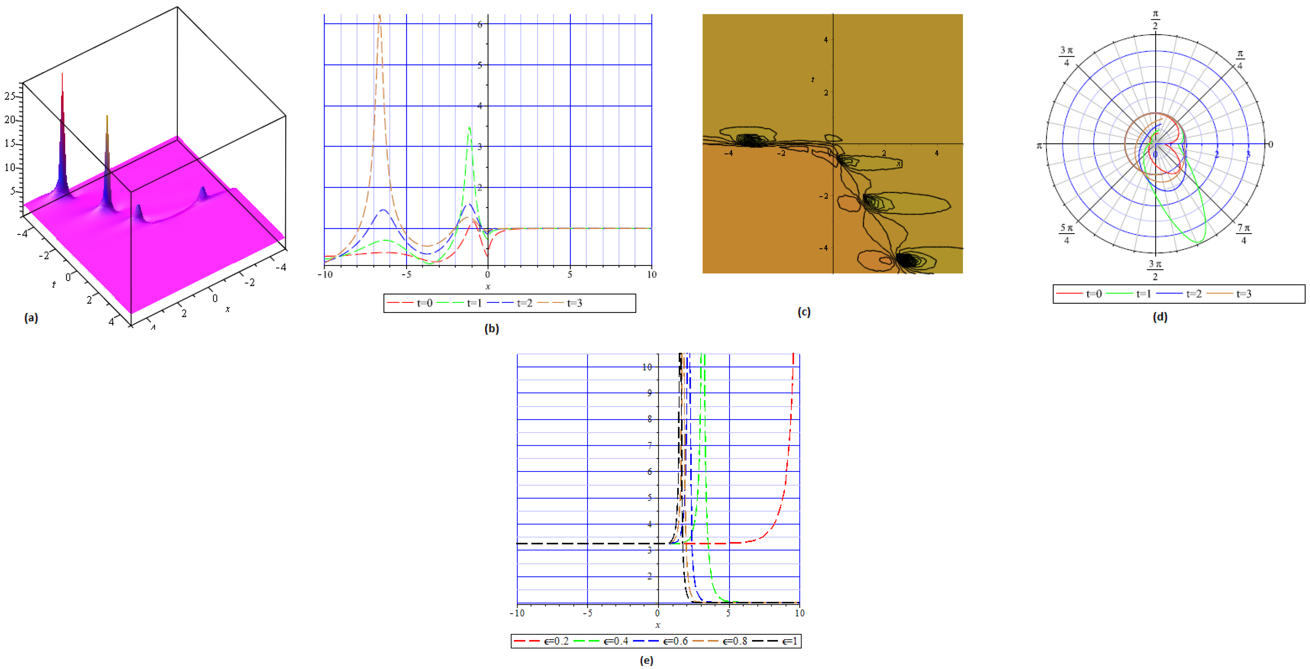
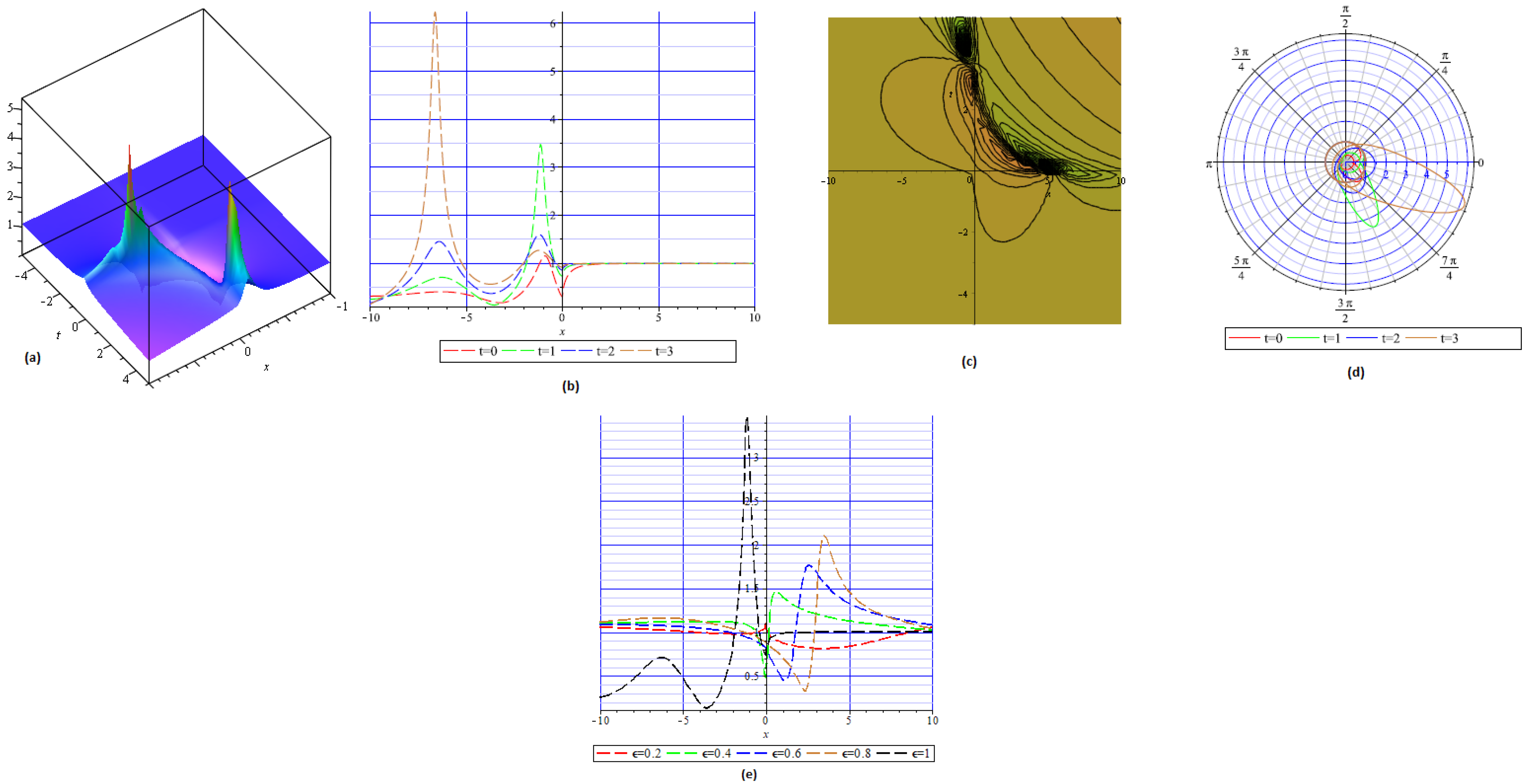
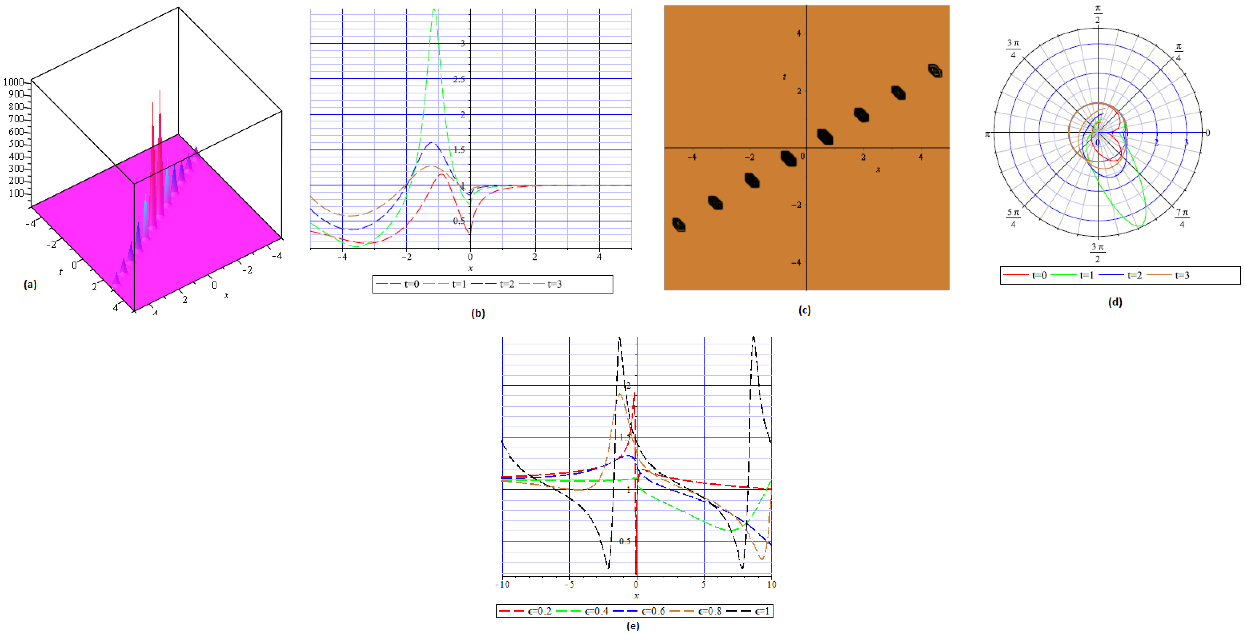
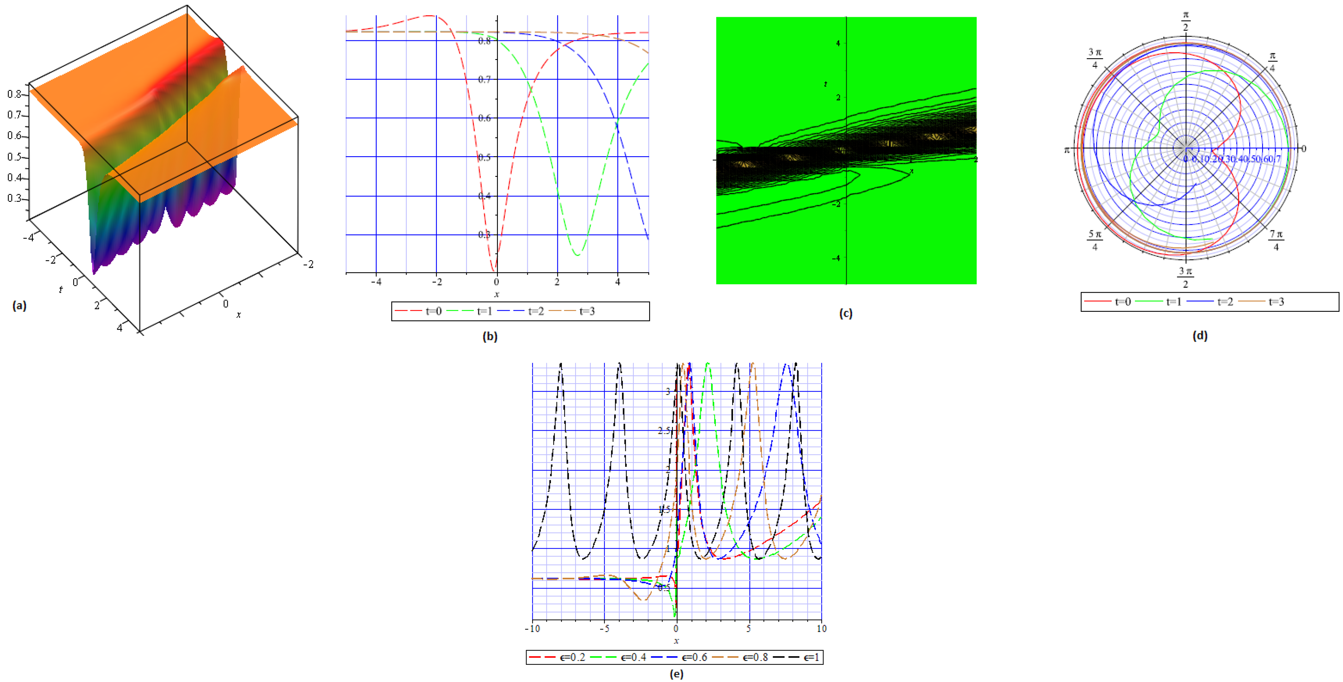
4. Physical Interpretation

This section presents the physical interpretation of the obtained solutions. Figure 1 shows the physical behavior of the appearance of solution Abs(h(x,t)) in Equation (24) with $ϵ=0.6,\varrho =2,\mu =0.5,\Omega =-0.1$ in (a) 3D, in (b) 2D, in (c) contour, in (d) polar form, and in (e) with fractional order $ϵ=0.2,0.4,0.6,0.8,1$. Figure 2 shows the physical behavior of the appearance of solution Abs(h(x,t)) in Equation (25) with $ϵ=0.6$, $\varrho =2$, $\mu =-1.5,\Omega =-1$ in (a) 3D, in (b) 2D, in (c) contour, in (d) polar form, and in (e) with fractional order $ϵ=0.2,0.4,0.6,0.8,1$. Figure 3 shows the physical behavior of the appearance of solution Abs(h(x,t)) in Equation (26) with $ϵ=0.8,\varrho =2,\mu =0.5,\Omega =0.1$ in (a) 3D, in (b) 2D, in (c) contour, in (d) polar form, and in (e) with fractional order $ϵ=0.2,0.4,0.6,0.8,1$. Figure 4 shows the physical behavior of that appearance of solution Abs(h(x,t)) in Equation (27) with $ϵ=0.6,\varrho =2,\mu =1.5,\Omega =-1$ in (a) 3D, in (b) 2D, in (c) contour, in (d) polar form, and in (e) with fractional order $ϵ=0.2,0.4,0.6,0.8,1$. Figure 5 shows the physical behavior of the appearance of solution Abs(h(x,t)) in Equation (145) with $ϵ=0.8,{\lambda }_0=0.2,{\lambda }_1=-3,\mu =0.5,C_1=1,C_2=0.3,\varrho =2$ in (a) 3D, in (b) 2D, in (c) contour, in (d) polar form, and in (e) with fractional order $ϵ=0.2,0.4,0.6,0.8,1$. Figure 6 shows the physical behavior of the appearance of solution Abs(h(x,t)) in Equation (146) with $ϵ=0.8,{\lambda }_0=-3,{\lambda }_1=-3,\mu =0.5,C_1=1,C_2=-0.3,\varrho =2$ in (a) 3D, in (b) 2D, in (c) contour, in (d) polar form, and in (e) with fractional order $ϵ=0.2,0.4,0.6,0.8,1$.

5. MI Analysis

Examination of a steady-state method for solving the FitzHugh–Nagumo model is shown in [22]:

$$h(x,t)=\left(H(x,t)+\sqrt{\tau }\right)e^{\iota \tau t},$$

(168)

where $\tau$ shows the optical normalizing power.

By using Equation (168) in Equation (1), by linearity we get

$$H^{(0,1)}(x,t)-H^{(2,0)}(x,t)+\theta H(x,t)+\iota \tau H(x,t)+\theta \sqrt{\tau }+\iota {\tau }^{3/2}=0.$$

(169)

Suppose the solution of Equation (169) is shown in [22], mentioned as:

$$H(x,t)=A_1{e}^{\iota (px-rt)}+A_2{e}^{-\iota (px-rt)}.$$

(170)

Here, “p” and “r” are the constants. Equation (170) is substituted into Equation (169). After solving the determinant of the coefficient matrix, we obtain the dispersion relation by adding the coefficients of $e^{\iota (px-rt)}$ and $e^{-\iota (px-rt)}$.

$${\theta }^2+p^4+2\theta p^2+r^2-{\tau }^2=0.$$

(171)

The dispersion relation can be found from Equation (171) for “r”, results

$$r=\pm \sqrt{-{\theta }^2-p^4-2\theta p^2+{\tau }^2}.$$

(172)

The steady-state stability is demonstrated by the gained dispersion relation. The steady-state outcome will not be stable when wave number q is not real because the perturbation increases exponentially. However, a steady state becomes stable against minor perturbations if q is not imaginary. The result is in the unstable steady state if

$$-{\theta }^2-p^4-2\theta p^2+{\tau }^2<0.$$

(173)

It is possible to acquire the MI gain spectrum $G\left(p\right)$ and shown in the Figure 7:

$$G\left(p\right)=2Im\left(r\right)=\pm \sqrt{-{\theta }^2-p^4-2\theta p^2+{\tau }^2}.$$

(174)

6. Conclusions

This paper contained the several kinds of exact wave solitons of the nonlinear FitzHugh–Nagumo model with a truncated M-fractional derivative. By using the modified extended tanh function technique and the modified $(G^{\prime }/G^2)$-expansion technique, we are able to obtain many more exact wave solitons, having kink, dark-bright, singular-periodic, periodic, bright, dark, singular, and complexiton solitons. The solutions differ from the current solutions due to the use of fractional derivatives. By using the fractional derivative, we obtained the solutions closer to the numerical solutions. The fractional derivative represents the concerned model in a more prominent form. In the very different domains of biosciences and telecommunications, especially in neural signal simulation and pulse control for optical communication, these solutions might be helpful. Contour graphs, two- and three-dimensional plots, are used to illustrate the obtained results. In addition, the stationary results of the governing equation are studied through modulation instability. Findings aid in the development of the relevant system. It is suggested that the techniques employed have applicability for other nonlinear equations in different scientific and engineering domains.

References

1. Raheel, M.; Zafar, A.; Razzaq, W.; Qousini, M. New analytical wave solitons and some other wave solutions of truncated M-fractional LPD equation along parabolic law of non-linearity. Opt. Quant. Electron. 2023, 55, 592. [Google Scholar] [CrossRef]
2. Qawaqneh, H.; Zafar, A.; Raheel, M.; Zaagan, A.A.; Zahran, E.H.M.; Cevikel, A.; Bekir, A. New soliton solutions of M-fractional Westervelt model in ultrasound imaging via two analytical techniques. Opt. Quant. Electron. 2024, 56, 737. [Google Scholar] [CrossRef]
3. Liu, C. The traveling wave solution and dynamics analysis of the fractional order generalized Pochhammer–Chree equation. AIMS Math. 2024, 9, 33956–33972. [Google Scholar] [CrossRef]
4. Mohammed, W.W.; Cesarano, C.; Iqbal, N.; Sidaoui, R.; E Ali, E. The exact solutions for the fractional Riemann wave equation in quantum mechanics and optics. Phys. Scr. 2024, 99, 085245. [Google Scholar] [CrossRef]
5. Razzaq, W.; Alsharidi, A.K.; Zafar, A.; Alomair, M.A. Optical solitons to the beta-fractional density dependent diffusion-reaction model via three different techniques. Int. J. Mod. Phys. B 2023, 37, 2350268. [Google Scholar] [CrossRef]
6. Abdou, M.A.; Soliman, A.A. Modified extended tanh-function method and its application on nonlinear physical equations. Phys. Lett. A 2006, 353, 487–492. [Google Scholar] [CrossRef]
7. Zahran, E.H.; Khater, M.M. Modified extended tanh-function method and its applications to the Bogoyavlenskii equation. Appl. Math. Model. 2016, 40, 1769–1775. [Google Scholar] [CrossRef]
8. Dubey, S.; Chakraverty, S. Application of modified extended tanh method in solving fractional order coupled wave equations. Math. Comput. Simul. 2022, 198, 509–520. [Google Scholar] [CrossRef]
9. Rabie, W.B.; Ahmed, H.M.; Darwish, A.; Hussein, H.H. Construction of new solitons and other wave solutions for a concatenation model using modified extended tanh-function method. Alex. Eng. J. 2023, 74, 445–451. [Google Scholar] [CrossRef]
10. Cinar, M.; Onder, I.; Secer, A.; Sulaiman, T.A.; Yusuf, A.; Bayram, M. Optical solitons of the (2+ 1)-dimensional Biswas–Milovic equation using modified extended tanh-function method. Optik 2021, 245, 167631. [Google Scholar] [CrossRef]
11. Behera, S.; Behera, D. Nonlinear wave dynamics of (1+1)-dimensional conformable coupled nonlinear Higgs equation using modified (G/G2)-expansion method. Phys. Scr. 2025. Available online: https://iopscience.iop.org/article/10.1088/1402-4896/adaa31 (accessed on 14 January 2025).
12. Saboor, A.; Shakeel, M.; Liu, X.; Zafar, A.; Ashraf, M.A. comparative study of two fractional nonlinear optical model via modified (G/G2)-expansion method. Opt. Quantum Electron. 2024, 56, 259. [Google Scholar] [CrossRef]
13. Aljahdaly, N.H. Some applications of the modified (G/G2)-expansion method in mathematical physics. Results Phys. 2019, 13, 102272. [Google Scholar] [CrossRef]
14. Cevikel, A.C.; Bekir, A.; Abu Arqub, O.; Abukhaled, M. Solitary wave solutions of Fitzhugh–Nagumo-type equations with conformable derivatives. Front. Phys. 2022, 10, 1028668. [Google Scholar] [CrossRef]
15. Tauseef Mohyud-Din, S.; Khan, Y.; Faraz, N.; Yıldırım, A. Exp-function method for solitary and periodic solutions of Fitzhugh-Nagumo equation. Int. J. Numer. Methods Heat Fluid Flow 2012, 22, 335–341. [Google Scholar] [CrossRef]
16. Yokus, A. On the exact and numerical solutions to the FitzHugh–Nagumo equation. Int. J. Mod. Phys. B 2020, 34, 2050149. [Google Scholar] [CrossRef]
17. Abdel-Aty, A.-H.; Khater, M.M.A.; Baleanu, D.; Khalil, E.M.; Bouslimi, J.; Omri, M. Abundant distinct types of solutions for the nervous biological fractional FitzHugh–Nagumo equation via three different sorts of schemes. Adv. Differ. Equ. 2020, 2020, 476. [Google Scholar] [CrossRef]
18. Sulaiman, T.A.; Yel, G.; Bulut, H. M-fractional solitons and periodic wave solutions to the Hirota-Maccari system. Mod. Phys. Lett. B 2019, 33, 1950052. [Google Scholar] [CrossRef]
19. Sousa, J.V.D.; Oliveira, E.C.D. A new truncated M-fractional derivative type unifying some fractional derivative types with classical properties. Int. J. Anal. Appl. 2018, 16, 83–96. [Google Scholar]
20. Raslan, K.R.; Khalid, K.A.; Shallal, M.A. The modified extended tanh method with the Riccati equation for solving the space-time fractional EW and MEW equations. Chaos Solitons Fractals 2017, 103, 404–409. [Google Scholar] [CrossRef]
21. Zhang, Y.; Zhang, L.; Pang, J. Application of (G/G2) Expansion Method for Solving Schrödinger’s Equation with Three-Order Dispersion. Adv. Appl. Math. 2017, 6, 212–217. [Google Scholar] [CrossRef]
22. ur Rehman, S.; Ahmad, J. Modulation instability analysis and optical solitons in birefringent fibers to RKL equation without four wave mixing. Alex. Eng. J. 2021, 60, 1339–1354. [Google Scholar] [CrossRef]
Figure 1. (Kink-like soliton) Physical behavior of solution’s appearance in Equation (24).
Fractalfract 09 00453 g001
Figure 2. (Dark soliton) Physical behavior of solution’s appearance in Equation (25).
Fractalfract 09 00453 g002
Figure 3. (Periodic soliton) Physical behavior of solution’s appearance in Equation (26).
Fractalfract 09 00453 g003
Figure 4. (Singular soliton) Physical behavior of solution’s appearance in Equation (27).
Fractalfract 09 00453 g004
Figure 5. (Kink soliton) Physical behavior of solution’s appearance in Equation (145).
Fractalfract 09 00453 g005
Figure 6. (Periodic wave solution) Physical behavior of solution’s appearance in Equation (146).
Fractalfract 09 00453 g006
Figure 7. MI gain spectrum at the values p = 1 , 2 , 3 , 4 and θ = 0.5 for τ [ 5 , 5 ] .
Fractalfract 09 00453 g007
Disclaimer/Publisher’s Note: The statements, opinions and data contained in all publications are solely those of the individual author(s) and contributor(s) and not of MDPI and/or the editor(s). MDPI and/or the editor(s) disclaim responsibility for any injury to people or property resulting from any ideas, methods, instructions or products referred to in the content.