Global Mittag-Leffler Synchronization of Fractional-Order Fuzzy Inertia Neural Networks with Reaction–Diffusion Terms Under Boundary Control

Abstract

This study is devoted to solving the global Mittag-Leffler synchronization problem of fractional-order fuzzy reaction–diffusion inertial neural networks by using boundary control. Firstly, the considered network model incorporates the inertia term, reaction–diffusion term and fuzzy logic, thereby enhancing the existing model framework. Secondly, to prevent an increase in the number of state variables due to the reduced-order approach, a non-reduced-order method is fully utilized. Additionally, a boundary controller is designed to lower resource usage. Subsequently, under the Neumann boundary condition, the mixed boundary condition and the Robin boundary condition, three synchronization conditions are established with the help of the non-reduced-order approach and LMI technique, respectively. Lastly, two numerical examples are offered to verify the reliability of the theoretical results and the availability of the boundary controller through MATLAB simulations.

1. Introduction

Neural networks (NNs) are a type of computational model based on the design idea of the biological nervous system. They are composed of a large number of interconnected artificial neurons and extract complex features from data through adaptive learning. Typical applications include computer vision [1], autonomous driving [2], natural language processing [3] and medical diagnosis [4]. Due to the specific characteristics of fractional calculus and its memory, heredity and nonlocal properties, for many real systems, it offers a more accurate description. Moreover, compared with traditional integer-order calculus, fractional-order calculus is more accurate in describing some dynamic processes, such as in population and industrial research [5,6]. Thus, it is natural to introduce fractional calculus into NNs [7,8,9,10,11]. Recently, synchronization, a key research focus in the field of NNs, has garnered extensive attention from numerous scholars. To date, a wealth of outstanding findings concerning the synchronization of fractional-order NNs have been documented [12,13,14,15,16].

However, NNs with first-order state derivatives tend to have constraints in addressing certain issues, such as chaotic memory searches, automatic tracking and secure communication. Hence, the introduction of an inertia term is an effective means to enhance the dynamic performance of the system [17,18]. Inertial NNs (INNs) were originally presented by Babcock and Westervelt in 1987 [19]. They represent a type of second-order delay differential equation, formed by incorporating an inertial term into multi-directional associative memory NNs. INNs, grounded in the Hopfield model, delve into the dynamic behaviors of second-order differential equations, including chaos and bifurcation. Recently, many scholars have made valuable contributions in this field [20,21,22]. All of the above methods are concentrated in the integer order, which restrains the ability to capture intricate dynamic behavior to some extent. In order to simulate the actual system’s dynamic behavior with greater accuracy and enhance the system’s degree of freedom, scholars have begun to study fractional-order INNs and achieved many interesting results. For example, through variable substitution, Cheng et al. gave a new synchronization criterion for fractional-order INNs [23]. The stability conditions of delay-dependent impulsive Caputo fractional-order INNs were given by the fractional Lyapunov functional method and the average impulsive delay in [24]. Li et al. analyzed the global Mittag-Leffler synchronization of fractional-order delayed Cohen–Grossberg INNs by applying the reduced order technique [25].

The above works focus on fractional-order INNs within a deterministic environment. In practical applications, fractional-order INNs often encounter challenges, such as complexity, nonlinearity and ambiguity [26], which may complicate theoretical analysis. In order to overcome this difficulty, it is meaningful to effectively combine the fuzzy operator with fractional-order INNs. Recently, some works on the synchronization of fractional-order fuzzy INNs have been reported [27,28]. Their successful application in the fields of control, prediction and diagnosis verify their theoretical superiority and engineering practicability. Thus, exploring the synchronization of fractional-order INNs with fuzzy rules holds significant theoretical and practical value.

In addition, in order to describe the dynamic behavior of the network more accurately, it is particularly important to consider the spatial diffusion characteristics—for example, the movement of electrons in an asymmetric magnetic field in artificial NNs [29,30,31], or material or energy migrating from a high-concentration region to a low-concentration region [32,33]. In recent decades, scholars have made a number of achievements in the study of fractional-order reaction–diffusion systems. For instance, under intermittent control, the bipartite synchronization of fractional-order T-S fuzzy heterogeneous reaction–diffusion NNs was studied [34]. In [35], Wang et al. discussed the passivity of fractional-order coupled NNs with reaction–diffusion terms and multiadaptive coupling and provided the passivity criterion. Employing the Lyapunov comparison principle, Wang et al. explored the stability and synchronization of fractional-order reaction–diffusion INNs (RDINNs) with parameter perturbations and time delays [36]. It is noted that the above works only consider a single state’s reaction–diffusion term. In fact, a single reaction–diffusion term cannot describe the nonlocality of the system and ignores the memory effects generated by dynamic processes, such as high-speed neural signal propagation [37] and non-Fourier heat conduction [38]. Therefore, it is essential to incorporate the reaction–diffusion term of the state derivative. Thus far, the synchronization of fractional-order fuzzy RDINNs (FOFRDINNs) has received relatively little attention, particularly in terms of studies that incorporate both states and state derivatives, which is the motivation of this research.

It is widely recognized that boundary control is an efficient and practical control strategy addressing the synchronization of reaction–diffusion NNs. The primary goal is to design a boundary controller that operates exclusively on the system’s spatial boundary, as opposed to regulating the entire system or requiring full-state feedback, thereby achieving synchronization. Boundary control was first proposed by Greenberg and Tsien in 1984 [39]. Based on this, boundary control has seen significant development when it comes to fractional-order reaction–diffusion NNs [40,41,42]. Under internal and boundary control, Shi et al. analyzed the fixed-time synchronization issue of complex reaction–diffusion networks with the Robin condition [40]. By designing an intermittent boundary controller, Liu et al. investigated the synchronization problem of fractional-order reaction–diffusion NNs in [41]. In order to study the synchronization problem of fractional-order delayed reaction–diffusion NNs with mixed boundary conditions, a boundary controller that only depends on the boundary conditions has been designed [42]. It is important to highlight that the above works have not applied boundary control to discuss the synchronization of FOFRDINNs. Thus, the synchronization problem concerning FOFRDINNs based on boundary control is worthy of further study.

Building on the previous discussion, this paper studies the global Mittag-Leffler synchronization issue of FOFRDINNs with the state’s reaction–diffusion term and the state derivative’s reaction–diffusion term under Neumann, mixed and Robin boundary conditions through appropriate the boundary controller. The core innovations of this work are presented as follows.

(1)

In view of the complexity of the actual network, fuzzy rules, the state’s reaction–diffusion term and the state derivative’s reaction–diffusion term are all introduced into the fractional-order INN model simultaneously, which is more general than the traditional fractional-order INN [23,24,25,27,28].

(2)

The original 2$\beta$-order system is regarded as a whole by employing the non-reduced technique in this paper, instead of splitting it into two $\beta$-order systems by virtue of the variable substitution approach [23,24,25]. In contrast to [23,24,25], the theoretical analysis is more concise.

(3)

Compared with the results considering only a single boundary condition [41,43], three types of synchronization criteria are obtained under the Neumann boundary condition, the mixed boundary condition and the Robin boundary condition. Thus, the theoretical framework is more comprehensive.

The structure of the remainder of this article is as follows. In Section 2, the model of FOFRDINNs is presented, along with some essential preliminary knowledge. In Section 3, the synchronization criteria under the three boundary conditions are given. In Section 4, corresponding numerical examples are provided to verify the effectiveness of the proposed control scheme. Finally, the conclusions of this article are given in Section 5.

Notations. $R=(-\infty ,+\infty )$, $\mathrm{diag}\{·\}$ represents a diagonal matrix, $R^n$ denotes the n-dimensional real Euclidean space, and $R^{n\times n}$ represents the $n\times n$ dimensional real matrix space. $\mathbf{0}\in R^{n\times n}$ denotes a matrix whose elements are all 0, $|\xi |=(|{\xi }_{ij}{|)}_{n\times n}\in R^{n\times n}$. $\parallel ·\parallel$ symbolizes the 2-norm of a vector, $P<0(>0)$ means that P is a negative (positive) definite matrix, and ${\lambda }_{min}\left(P\right)$ stands for the minimum eigenvalue of P.

2. Preliminaries and Model Description

2.1. Fractional Calculus Definition and Properties

Definition 1

([44]). The β-order Caputo fractional derivative of a function $h\left(t\right)(t\ge t_0)$ is given by

$$\begin{array}{c}\hfill D_{t_0}^{\beta }h\left(t\right)={\displaystyle \frac{1}{\mathrm{\Gamma }(1-\beta )}}{\int }_{t_0}^t{\displaystyle \frac{h^{\prime }\left(\tau \right)}{{(t-\tau )}^{\beta }}}d\tau ,\end{array}$$

where $h\left(t\right):[t_0,+\infty )\to R,\mathrm{\Gamma }(·)$ denotes the Gamma function and $0<\beta <1$.

Definition 2

([44]). The Caputo fractional derivative of $h(t,s)$ is defined as

$$\begin{array}{c}\hfill {\displaystyle \frac{{\partial }^{\beta }h(t,s)}{\partial t^{\beta }}}={\displaystyle \frac{1}{\mathrm{\Gamma }(1-\beta )}}{\int }_{t_0}^t{(t-\tau )}^{-\beta }{\displaystyle \frac{\partial h(\tau ,s)}{\partial \tau }}d\tau ,\end{array}$$

where $h(t,s):[0,+\infty )\times [0,l]\to R,\mathrm{\Gamma }(·)$ denotes the Gamma function and $0<\beta <1$.

Definition 3

([44]). The Mittag-Leffler function of one parameter is defined as

$$\begin{array}{c}\hfill E_{\beta }\left(t\right)=\sum _{k=1}^{+\infty }{\displaystyle \frac{t^k}{\mathrm{\Gamma }(\beta k+1)}},\beta \in (0,1),t\in R.\end{array}$$

Lemma 1

([45]). Let $\delta (t,s):[0,+\infty )\times [0,l]\to R$ be continuously differentiable with respect to t; then,

$$\begin{array}{c}\hfill {\displaystyle \frac{{\partial }^{\beta }}{\partial t^{\beta }}}\left[\delta {(t,s)}^T\delta (t,s)\right]\le 2\delta {(t,s)}^T{\displaystyle \frac{{\partial }^{\beta }}{\partial t^{\beta }}}\delta (t,s),\beta \in (0,1).\end{array}$$

Lemma 2

([40]). For any continuous function $\delta (t,s):[0,+\infty )\times [0,l]\to R$ satisfying $\delta (t,0)=0$ or $\delta (t,l)=0$, and for any matrix $D>0$,

$$\begin{array}{c}\hfill {\int }_0^l\delta {(t,s)}^{T}D\delta (t,s)ds\le {\displaystyle \frac{4l^2}{{\pi }^2}}{\int }_0^l{\displaystyle \frac{\partial \delta {(t,s)}^T}{\partial s}}D{\displaystyle \frac{\partial \delta (t,s)}{\partial s}}ds.\end{array}$$

Lemma 3

([45]). Suppose that $\delta (t,s):[0,+\infty )\times [0,l]\to R$ is continuously differentiable with respect to t; then, for any $a,b\in R,\beta \in (0,1),$

$$\begin{array}{c}\hfill {\displaystyle \frac{{\partial }^{\beta }}{\partial t^{\beta }}}(a\delta (t,s)+b\delta (t,s))=a{\displaystyle \frac{{\partial }^{\beta }\delta (t,s)}{\partial t^{\beta }}}+b{\displaystyle \frac{{\partial }^{\beta }\delta v(t,s)}{\partial t^{\beta }}}.\end{array}$$

Lemma 4

([45]). For any continuously differentiable function $\mathcal{V}\left(t\right):[0,+\infty )\to R$, if there exists a constant $\sigma \in R$ such that

$$\begin{array}{c}\hfill D_{t_0}^{\beta }\mathcal{V}\left(t\right)\le \sigma \mathcal{V}\left(t\right),\end{array}$$

then

$$\mathcal{V}\left(t\right)\le \mathcal{V}\left(0\right)E_{\beta }\left(\sigma t^{\beta }\right).$$

Lemma 5

([46]). For any $y_1,y_2,{\xi }_{ij},{\eta }_{ij}\in R$, and $f_j(·)$ is a continuous function; then,

$$\begin{array}{c}\hfill |\underset{j=1}{\overset{n}{\bigwedge }}{\xi }_{ij}{f}_j\left(y_1\right)-\underset{j=1}{\overset{n}{\bigwedge }}{\xi }_{ij}{f}_j\left(y_2\right)|\le \sum _{j=1}^n|{\xi }_{ij}||f_j\left(y_1\right)-f_j\left(y_2\right)|,\end{array}$$

$$\begin{array}{c}\hfill |\underset{j=1}{\overset{n}{\bigvee }}{\eta }_{ij}{f}_j\left(y_1\right)-\underset{j=1}{\overset{n}{\bigvee }}{\eta }_{ij}{f}_j\left(y_2\right)|\le \sum _{j=1}^n|{\eta }_{ij}||f_j\left(y_1\right)-f_j\left(y_2\right)|.\end{array}$$

Lemma 6

([47]). Suppose that $v(t,s)$ is differentiable with respect to t and integrable on $[0,l]$. Let

$$\begin{array}{c}\hfill G(t,s)={\int }_0^{l}v(t,s)ds,\end{array}$$

and then

$$\begin{array}{c}\hfill {\displaystyle \frac{{\partial }^{\beta }G(t,s)}{\partial t^{\beta }}}={\int }_0^l{\displaystyle \frac{{\partial }^{\beta }v(t,s)}{\partial t^{\beta }}}ds.\end{array}$$

Lemma 7.

Let $v(t,s):[0,+\infty )\times [0,l]\to R$ be continuously differentiable; then, for any $(t,s)\in [0,+\infty )\times [0,l],$

$$\begin{array}{c}\hfill {\displaystyle \frac{{\partial }^{\beta }}{\partial t^{\beta }}}\left({\displaystyle \frac{\partial v(t,s)}{\partial s}}\right)={\displaystyle \frac{\partial }{\partial s}}\left({\displaystyle \frac{{\partial }^{\beta }v(t,s)}{\partial t^{\beta }}}\right).\end{array}$$

Proof. 

By Definition 2, this yields

$$\begin{array}{cc}\hfill {\displaystyle \frac{{\partial }^{\beta }}{\partial t^{\beta }}}\left({\displaystyle \frac{\partial v(t,s)}{\partial s}}\right)=& {\displaystyle \frac{1}{\mathrm{\Gamma }(1-\beta )}}{\int }_0^t{(t-\tau )}^{-\beta }{\displaystyle \frac{\partial }{\partial \tau }}\left({\displaystyle \frac{\partial v(\tau ,s)}{\partial s}}\right)d\tau \hfill \\ \hfill =& {\displaystyle \frac{1}{\mathrm{\Gamma }(1-\beta )}}{\int }_0^t{(t-\tau )}^{-\beta }{\displaystyle \frac{\partial }{\partial s}}\left({\displaystyle \frac{\partial v(\tau ,s)}{\partial \tau }}\right)d\tau \hfill \\ \hfill =& {\displaystyle \frac{1}{\mathrm{\Gamma }(1-\beta )}}{\displaystyle \frac{\partial }{\partial s}}{\int }_0^t{(t-\tau )}^{-\beta }\left({\displaystyle \frac{\partial v(\tau ,s)}{\partial \tau }}\right)d\tau \hfill \\ \hfill =& {\displaystyle \frac{\partial }{\partial s}}\left({\displaystyle \frac{{\partial }^{\beta }v(t,s)}{\partial t^{\beta }}}\right).\hfill \end{array}$$

□

2.2. Model Description

Consider a class of FOFRDINNs, which are modeled as

$$\begin{array}{cc}\hfill {\displaystyle \frac{{\partial }^{\beta }}{\partial t^{\beta }}}\left({\displaystyle \frac{{\partial }^{\beta }{z}_i(t,s)}{\partial t^{\beta }}}\right)=& -k_i{\displaystyle \frac{{\partial }^{\beta }{z}_i(t,s)}{\partial t^{\beta }}}+d_i{\Delta }_i{z}_i(t,s)+\overline{d_i}{\Delta }_i{\displaystyle \frac{{\partial }^{\beta }{z}_i(t,s)}{\partial t^{\beta }}}-a_i{z}_i(t,s)\hfill \\ \hfill & +\sum _{j=1}^n{b}_{ij}{f}_j\left(z_j(t,s)\right)+\sum _{j=1}^n{T}_{ij}{\chi }_j+\underset{j=1}{\overset{n}{\bigwedge }}{Q}_{ij}{\chi }_j+\underset{j=1}{\overset{n}{\bigvee }}{H}_{ij}{\chi }_j\hfill \\ \hfill & +\underset{j=1}{\overset{n}{\bigwedge }}{\xi }_{ij}{f}_j\left(z_j(t,s)\right)+\underset{j=1}{\overset{n}{\bigvee }}{\eta }_{ij}{f}_j\left(z_j(t,s)\right)+I_i\left(t\right),\hfill \end{array}$$

(1)

where $\beta \in (0,1),i\in \mathcal{I}=\{1,2,\cdots ,n\}$, n represents the number of neurons, $z_i(t,s)\in R$ is the state of ith neuron at time t and position s, $f_j(t,s)$ denotes the activation function, ${\displaystyle \frac{{\partial }^{\beta }}{\partial t^{\beta }}}\left({\displaystyle \frac{{\partial }^{\beta }{z}_i}{\partial t^{\beta }}}\right)$ stands for the inertial term, ${\Delta }_i={\displaystyle \frac{{\partial }^2}{\partial s^2}}$ is the diffusion term, and $d_i$ and $\overline{d_i}$ indicate the spacial diffusion coefficients along the ith neuron. The constant $k_i$ corresponds to a specific value. The rate at which the ith unit returns its potential to the resting state when isolated is represented by $a_i$. The synaptic connection weight from the jth unit to the ith unit is denoted by $b_{ij}$. ⋀ and ⋁ represent the operations of fuzzy OR and fuzzy AND. $Q_{ij},H_{ij},{\xi }_{ij}$ and ${\eta }_{ij}$ are the state parameters of fuzzy MIN feedforward, fuzzy MAX feedforward, fuzzy MIN feedback and fuzzy MAX feedback, respectively. $T_{ij}$ signifies the feedforward template, ${\chi }_j$ is the input of the jth neuron, and $I_i\left(t\right)$ is the external bias of the jth neuron.

The initial values associated with system (1) are

$$\begin{array}{c}\hfill z_i(0,x)={\varphi }_i(0,s),{\displaystyle \frac{{\partial }^{\beta }{z}_i(0,s)}{\partial t^{\beta }}}={\psi }_i(0,s),x\in [0,l],\end{array}$$

(2)

and the Robin boundary condition of system (1) is provided by

$$\begin{array}{c}\hfill \left\{\begin{array}{c}{\rho }_1{\displaystyle \frac{\partial z_i(t,s)}{\partial s}}{{|}_{s=0}+{\overline{\rho }}_1{z}_i(t,s)|}_{s=0}=0,t\in [0,+\infty ),\hfill \\ {\rho }_2{\displaystyle \frac{\partial z_i(t,s)}{\partial s}}{{|}_{s=l}+{\overline{\rho }}_2{z}_i(t,s)|}_{s=l}=0,t\in [0,+\infty ),\hfill \end{array}\right.\end{array}$$

(3)

where ${\rho }_1,{\overline{\rho }}_1,{\rho }_2,{\overline{\rho }}_2\in R$.

Remark 1.

Compared with the previous research on fractional-order INNs [24,25,27,28], this paper innovatively integrates the reaction–diffusion effects of both the state and its derivative in INNs, offering a more precise description of the reaction–diffusion phenomenon in the realms of physics and biology. Thus, the mathematical model presented in this study enriches the research on fractional-order INNs. In particular, when the inertia term is not considered, the system simplifies to the models in [35,41]. Additionally, the Robin boundary condition, which incorporates both the Neumann and Dirichlet boundary conditions, can be seen as a unified version of relevant results [41,48].

Remark 2.

It is easy to see that, when $0<\beta <0.5$, one has ${\displaystyle \frac{{\partial }^{\beta }}{\partial t^{\beta }}}{\displaystyle \frac{{\partial }^{\beta }{z}_i(t,s)}{\partial t^{\beta }}}={\displaystyle \frac{{\partial }^{2\beta }{z}_i(t,s)}{\partial t^{2\beta }}}$, but, when $0.5<\beta <1$, the Caputo fractional derivative does not satisfy the law of operation. Thus, the equation ${\displaystyle \frac{{\partial }^{\beta }}{\partial t^{\beta }}}{\displaystyle \frac{{\partial }^{\beta }{z}_i(t,s)}{\partial t^{\beta }}}={\displaystyle \frac{{\partial }^{2\beta }{z}_i(t,s)}{\partial t^{2\beta }}}$ is not valid. For example, ${\displaystyle \frac{{\partial }^{0.6}}{\partial t^{0.6}}}{\displaystyle \frac{{\partial }^{0.6}(t+s)}{\partial t^{0.6}}}={\displaystyle \frac{1}{\mathrm{\Gamma }\left(0.8\right)}}{t}^{-0.2},{\displaystyle \frac{{\partial }^{1.2(t+s)}}{\partial t^{1.2}}}=0.$

Taking system (1) as the drive system, the corresponding response system is expressed by

$$\begin{array}{cc}\hfill {\displaystyle \frac{{\partial }^{\beta }}{\partial t^{\beta }}}\left({\displaystyle \frac{{\partial }^{\beta }{w}_i(t,s)}{\partial t^{\beta }}}\right)=& -k_i{\displaystyle \frac{{\partial }^{\beta }{w}_i(t,s)}{\partial t^{\beta }}}+d_i{\Delta }_i{w}_i(t,s)+\overline{d_i}{\Delta }_i{\displaystyle \frac{{\partial }^{\beta }{w}_i(t,s)}{\partial t^{\beta }}}-a_i{w}_i(t,s)\hfill \\ \hfill & +\sum _{j=1}^n{b}_{ij}{f}_j\left(w_j(t,s)\right)+\sum _{j=1}^n{T}_{ij}{\chi }_j+\underset{j=1}{\overset{n}{\bigwedge }}{Q}_{ij}{\chi }_j+\underset{j=1}{\overset{n}{\bigvee }}{H}_{ij}{\chi }_j\hfill \\ & +\underset{j=1}{\overset{n}{\bigwedge }}{\xi }_{ij}{f}_j\left(w_j(t,s)\right)+\underset{j=1}{\overset{n}{\bigvee }}{\eta }_{ij}{f}_j\left(w_j(t,s)\right)+I_i\left(t\right)+u_i\left(t\right),\hfill \end{array}$$

(4)

where $u_i\left(t\right)$ denotes the control input.

The initial values of system (4) are

$$\begin{array}{c}\hfill w_i(0,s)=\widetilde{{\varphi }_i}(0,s),{\partial }_t^{\beta }{w}_i(0,s)=\widetilde{{\psi }_i}(0,s),s\in (0,l],\end{array}$$

(5)

and the Robin boundary condition of system (4) is offered as

$$\begin{array}{c}\hfill \left\{\begin{array}{c}{\rho }_1{\displaystyle \frac{\partial w_i(t,s)}{\partial s}}{{|}_{s=0}+{\overline{\rho }}_1{w}_i(t,s)|}_{s=0}=0,t\in [0,+\infty ),\hfill \\ {\rho }_2{\displaystyle \frac{\partial w_i(t,s)}{\partial s}}{{|}_{s=l}+{\overline{\rho }}_2{w}_i(t,s)|}_{s=l}=u_i\left(t\right),t\in [0,+\infty ).\hfill \end{array}\right.\end{array}$$

(6)

Define $v_i(t,s)=w_i(t,s)-z_i(t,s)$ as the synchronization error, and the error system can be described by

$$\begin{array}{cc}\hfill {\partial }_t^{\beta }\left({\partial }_t^{\beta }{v}_i(t,s)\right)=& -k_i{\partial }_t^{\beta }{v}_i(t,s)+d_i{\Delta }_i{v}_i(t,s)+\overline{d_i}{\Delta }_i\left({\partial }_t^{\beta }{v}_i(t,s)\right)\hfill \\ \hfill & -a_i{v}_i(t,s)+\sum _{j=1}^n{b}_{ij}{f}_j\left(v_j(t,s)\right)+\underset{j=1}{\overset{n}{\bigwedge }}{\xi }_{ij}{f}_j\left(v_j(t,s)\right)\hfill \\ \hfill & +\underset{j=1}{\overset{n}{\bigvee }}{\eta }_{ij}{f}_j\left(v_j(t,s)\right)+u_i\left(t\right).\hfill \end{array}$$

(7)

The initial values of system (7) are given by

$$\begin{array}{c}\hfill v_i(0,s)=\overline{{\varphi }_i}(0,s),{\partial }_t^{\beta }{v}_i(0,s)=\overline{{\psi }_i}(0,s),s\in (0,l],\end{array}$$

(8)

and the form of the Robin boundary condition for system (7) is as follows:

$$\begin{array}{c}\hfill \left\{\begin{array}{c}{\rho }_1{\partial }_s{v}_i(t,s){{|}_{s=0}+{\overline{\rho }}_1{v}_i(t,s)|}_{s=0}=0,t\in [0,+\infty ),\hfill \\ {\rho }_2{\partial }_s{v}_i(t,s){{|}_{s=l}+{\overline{\rho }}_2{v}_i(t,s)|}_{s=l}=u_i\left(t\right),t\in [0,+\infty ),\hfill \end{array}\right.\end{array}$$

(9)

where $f_j\left(v_j(t,s)\right)=f_j\left(w_j(t,s)\right)-f_j\left(z_j(t,s)\right)$, ${\overline{\varphi }}_i(0,s)={\tilde{\varphi }}_i(0,s)-{\varphi }_i(0,s)$, ${\overline{\psi }}_i(0,s)={\tilde{\psi }}_i(0,s)-{\psi }_i(0,s).$

For ease of analysis, let ${\partial }_t^{\beta }v(t,s)={\displaystyle \frac{{\partial }^{\beta }v(t,s)}{\partial t^{\beta }}},{\partial }_{s}v(t,s)={\displaystyle \frac{\partial v(t,s)}{\partial s}}$; we give the following compact form of error system (7):

$$\begin{array}{cc}\hfill {\partial }_t^{\beta }\left({\partial }_t^{\beta }v(t,s)\right)=& -K{\partial }_t^{\beta }v(t,s)+D_1\Delta v(t,s)+D_2\Delta \left({\partial }_{t}v(t,s)\right)-Av(t,s)\hfill \\ \hfill & +Bf\left(v\right(t,s\left)\right)+\xi \ast f\left(v\right(t,s\left)\right)+\eta ·f\left(v\right(t,s\left)\right)+u\left(t\right),\hfill \end{array}$$

(10)

where $K=\mathrm{diag}\{k_1,k_2,\dots ,k_n\},D_1=\mathrm{diag}\{d_1,d_2,\dots ,d_n\},A=\mathrm{diag}\{a_1,a_2,\dots ,a_n\}$ $B={\left(b_{ij}\right)}_{n\times n},\xi ={\left({\xi }_{ij}\right)}_{n\times n},\eta ={\left({\eta }_{ij}\right)}_{n\times n},v(t,s)={(v_1(t,s),v_2(t,s),\dots ,v_n(t,s))}^T,D_2=\mathrm{diag}\{\overline{d_1},\overline{d_2},\dots ,\overline{d_n}\},f\left(v(t,s)\right)={(f_1\left(v_1(t,s)\right),f_2\left(v_2(t,s)\right),\dots ,f_n\left(v_n(t,s)\right))}^T,\xi \ast f\left(v(t,s)\right)={({\bigwedge }_{j=1}^n{\xi }_{1j}{f}_j\left(v_j(t,s)\right),{\bigwedge }_{j=1}^n{\xi }_{2j}{f}_j\left(v_j(t,s)\right),\dots ,{\bigwedge }_{j=1}^n{\xi }_{nj}{f}_j\left(v_j(t,s)\right))}^T,\eta ·f\left(v(t,s)\right)={({\bigvee }_{j=1}^n{\xi }_{1j}{f}_j\left(v_j(t,s)\right),{\bigvee }_{j=1}^n{\xi }_{2j}{f}_j\left(v_j(t,s)\right),\dots ,{\bigvee }_{j=1}^n{\xi }_{nj}{f}_j\left(v_j(t,s)\right))}^T,u\left(t\right)={(u_1\left(t\right),u_2\left(t\right),\dots ,u_n\left(t\right))}^T.$

The initial values related to system (10) are

$$\begin{array}{c}\hfill v(0,s)=\overline{\varphi }(0,s),{\partial }_t^{\beta }v(0,s)=\overline{\psi }(0,s),s\in (0,l],\end{array}$$

(11)

and the Robin boundary conditions of system (10) are provided by

$$\begin{array}{c}\hfill \left\{\begin{array}{c}{\rho }_1{\partial }_{s}v(t,s){{|}_{s=0}+{\overline{\rho }}_{1}v(t,s)|}_{s=0}={\mathbf{0}}_n,t\in [0,+\infty ),\hfill \\ {\rho }_2{\partial }_{s}v(t,s){{|}_{s=l}+{\overline{\rho }}_{2}v(t,s)|}_{s=l}=u\left(t\right),t\in [0,+\infty ),\hfill \end{array}\right.\end{array}$$

(12)

where $\overline{\varphi }(0,s)={({\overline{\varphi }}_1(0,s),{\overline{\varphi }}_2(0,s),\dots ,{\overline{\varphi }}_n(0,s))}^T,\overline{\psi }(0,s)={({\overline{\psi }}_1(0,s),{\overline{\psi }}_2(0,s),\dots ,{\overline{\psi }}_n(0,s))}^T.$

Definition 4

([45]). Systems (1) and (4) are said to be globally Mittag-Leffler synchronized if there exist constants $M>0$ and $\sigma >0$ such that

$$\begin{array}{c}\hfill ||v(t,s)||\le M{E}_{\beta }(-\sigma t^{\beta }).\end{array}$$

Assumption 1.

For any $h_1,h_2\in R$, there exists a constant ${\theta }_i$ such that

$$|f_i\left(h_1\right)-f_i\left(h_2\right)|\le {\theta }_i|h_1-h_2|,i=1,2,\dots ,n.$$

3. Main Results

In this section, the synchronization issue of FOFRDINNs is analyzed under three different boundary conditions.

3.1. Synchronization Analysis Under Neumann Boundary Condition

When ${\rho }_1={\rho }_2=1$ and ${\overline{\rho }}_1={\overline{\rho }}_2=0$, the boundary condition (3) is reduced to the following Neumann boundary condition:

$$\begin{array}{c}\hfill {\partial }_s{z}_i(t,s){{|}_{s=0}=0,{\partial }_s{z}_i(t,s)|}_{s=l}=0,t\in [0,+\infty ).\end{array}$$

(13)

The boundary condition (6) degenerates into

$$\begin{array}{c}\hfill {\partial }_s{w}_i(t,s){{|}_{x=0}=0,{\partial }_s{w}_i(t,s)|}_{s=l}=u_i\left(t\right),t\in [0,+\infty ).\end{array}$$

(14)

In order to enable systems (1) and (4) to achieve synchronization, we propose the following boundary control strategy:

$$\begin{array}{c}\hfill u\left(t\right)=P{\int }_0^{l}v(t,s)ds,\end{array}$$

(15)

where $P=\mathrm{diag}\{P_1,P_2,\dots ,P_n\}(P_i<0)$ is the control gain.

Theorem 1.

Under Assumption 1 and controller (15), systems (1) and (4) with Neumann boundary conditions (13) and (14) can reach global Mittag-Leffler synchronization if there exist a constant $\epsilon >0$ and a matrix $P\in R^{n\times n}$ satisfying

$$\begin{array}{c}\hfill \Omega =\left(\begin{array}{ccccc}2D_{2}P+\Phi & *& *& *& *\\ -D_{2}P& -{\displaystyle \frac{{\pi }^2}{2l^2}}{D}_2& *& *& *\\ -D_{2}P& \mathbf{0}& -{\displaystyle \frac{{\pi }^2}{4l^2}}{D}_1& *& *\\ (D_1-D_2)P& -(D_1-D_2)P& -(D_1-D_2)P& \Psi & *\\ \mathbf{0}& \mathbf{0}& \mathbf{0}& \mathbf{0}& -D_1\end{array}\right)<0,\end{array}$$

(16)

$$\begin{array}{c}\hfill -\epsilon I+I+A-K\le 0,\end{array}$$

(17)

where $\Phi =B{B}^T+{|\xi ||\xi |}^T+{|\eta ||\eta |}^T+\epsilon I+I-A-K,\Psi =-\epsilon I-I-A+K+3\theta$.

Proof. 

Choose the Lyapunov function

$$\begin{array}{c}\hfill \mathcal{V}\left(t\right)={\mathcal{V}}_1\left(t\right)+{\mathcal{V}}_2\left(t\right)+{\mathcal{V}}_3\left(t\right),\end{array}$$

(18)

where

$$\begin{array}{cc}\hfill & {\mathcal{V}}_1\left(t\right)={\int }_0^l{\left(v(t,s)+{\partial }_t^{\beta }v(t,s)\right)}^T\left(v(t,s)+{\partial }_t^{\beta }v(t,s)\right)ds,\hfill \\ \hfill & {\mathcal{V}}_2\left(t\right)=\epsilon {\int }_0^{l}v{(t,s)}^{T}v(t,s)ds,\hfill \\ \hfill & {\mathcal{V}}_3\left(t\right)={\int }_0^l{\left({\partial }_{s}v(t,s)\right)}^T(D_1+D_2)\left({\partial }_{s}v(t,s)\right)ds.\hfill \end{array}$$

For simplicity, let $v=v(t,s),{\partial }_t^{\beta }v={\partial }_t^{\beta }v(t,s),{\partial }_{s}v={\partial }_{s}v(t,s),f\left(v\right)=f\left(v(t,s)\right)$. Lemmas 1 and 2 give

$$\begin{array}{cc}\hfill {\displaystyle \frac{{\partial }^{\beta }{\mathcal{V}}_1\left(t\right)}{\partial t^{\beta }}}\le & 2{\int }_0^l{\left(v+{\partial }_t^{\beta }v\right)}^T\left({\partial }_t^{\beta }v+{\partial }_t^{\beta }\left({\partial }_t^{\beta }v\right)\right)ds\hfill \\ \hfill =& 2{\int }_0^l{\left(v+{\partial }_t^{\beta }v\right)}^T({\partial }_t^{\beta }v-K{\partial }_t^{\beta }v+D_1\Delta v+D_2\Delta {\partial }_{t}v-Av\hfill \\ \hfill & +Bf\left(v\right)+Cf\left(v\right)+\xi \ast f\left(v\right)+\eta ·f\left(v\right))ds\hfill \\ \hfill \le & 2{\int }_0^l[{\left(v+{\partial }_t^{\beta }v\right)}^T(I-K){\partial }_t^{\beta }v+{\left(v+{\partial }_t^{\beta }v\right)}^T{D}_1{\partial }_s\left({\partial }_{s}v\right)\hfill \\ \hfill & +{\left(v+{\partial }_t^{\beta }v\right)}^T{D}_2{\partial }_s\left({\partial }_s{\partial }_t^{\beta }v\right)-{\left(v+{\partial }_t^{\beta }v\right)}^{T}Av\hfill \\ \hfill & +{\left(v+{\partial }_t^{\beta }v\right)}^{T}Bf\left(v\right)+{\left(v+{\partial }_t^{\beta }v\right)}^T(\xi \ast f\left(v\right))\hfill \\ \hfill & +{\left(v+{\partial }_t^{\beta }v\right)}^T(\eta ·g\left(v\right))]ds\hfill \end{array}$$

(19)

By Assumption 1 and $2{\mathbf{X}}^T\mathbf{Y}\le {\mathbf{X}}^T\mathbf{X}+{\mathbf{Y}}^T\mathbf{Y}$, one has

$$\begin{array}{cc}\hfill & 2{\left(v+{\partial }_t^{\beta }v\right)}^{T}Bf\left(v\right)\hfill \\ \hfill \le & {\left(v+{\partial }_t^{\beta }v\right)}^{T}B{B}^T\left(v+{\partial }_t^{\beta }v\right)+f^T\left(v\right)f\left(v\right)\hfill \\ \hfill \le & {\left(v+{\partial }_t^{\beta }v\right)}^{T}B{B}^T\left(v+{\partial }_t^{\beta }v\right)+v^T\theta v,\hfill \end{array}$$

(20)

$$\begin{array}{cc}\hfill & 2{\left(v+{\partial }_t^{\beta }v\right)}^T(\xi \ast f\left(v\right))\hfill \\ \hfill \le & {\left(v+{\partial }_t^{\beta }v\right)}^T{|\xi ||\xi |}^T\left(v+{\partial }_t^{\beta }v\right)+f^T\left(v\right)f\left(v\right)\hfill \\ \hfill \le & {\left(v+{\partial }_t^{\beta }v\right)}^T{|\xi ||\xi |}^T\left(v+{\partial }_t^{\beta }v\right)+v^T\theta v,\hfill \end{array}$$

(21)

$$\begin{array}{cc}\hfill & 2{\left(v+{\partial }_t^{\beta }v\right)}^T(\eta ·f\left(v\right))\hfill \\ \hfill \le & {\left(v+{\partial }_t^{\beta }v\right)}^T{|\eta ||\eta |}^T\left(v+{\partial }_t^{\beta }v\right)+f^T\left(v\right)f\left(v\right)\hfill \\ \hfill \le & {\left(v+{\partial }_t^{\beta }v\right)}^T{|\eta ||\eta |}^T\left(v+{\partial }_t^{\beta }v\right)+v^T\theta v,\hfill \end{array}$$

(22)

where $\theta =\mathrm{diag}\{{\theta }_1^2,{\theta }_2^2,\dots ,{\theta }_n^2\}$. Substituting (20)–(22) into (19), we have

$$\begin{array}{cc}\hfill {\displaystyle \frac{{\partial }^{\beta }{\mathcal{V}}_1\left(t\right)}{\partial t^{\beta }}}\le & {\int }_0^{l}2{\left({\partial }_t^{\beta }v\right)}^T(I-K){\partial }_t^{\beta }vds+{\int }_0^{l}2v^T(-A+I-K){\partial }_t^{\beta }vds\hfill \\ \hfill & +{\int }_0^l{\left(v+{\partial }_t^{\beta }v\right)}^T(B{B}^T+{|\xi ||\xi |}^T+{|\eta ||\eta |}^T)\left(v+{\partial }_t^{\beta }v\right)ds\hfill \\ \hfill & +{\int }_0^l{v}^T(-2A+3\theta )vds+{\int }_0^{l}2{\left(v+{\partial }_t^{\beta }v\right)}^T{D}_1{\partial }_s\left({\partial }_{s}v\right)ds\hfill \\ \hfill & +{\int }_0^{l}2{\left(v+{\partial }_t^{\beta }v\right)}^T{D}_2{\partial }_s\left({\partial }_s\left({\partial }_t^{\beta }v\right)\right)ds,\hfill \end{array}$$

(23)

From the Neumann boundary conditions (13) and (14), we have

$$\begin{array}{cc}\hfill & {\int }_0^l{\left(v+{\partial }_t^{\beta }v\right)}^T{D}_1{\partial }_s\left({\partial }_{s}v\right)ds\hfill \\ \hfill =& -{\int }_0^l{\left({\partial }_{s}v+{\partial }_s\left({\partial }_t^{\beta }v\right)\right)}^T{D}_1{\partial }_{s}vds+{\left(v+{\partial }_t^{\beta }v\right)}^T{D}_1{\partial }_{s}v{|}_{s=0}^{s=l}\hfill \\ \hfill =& -{\int }_0^l{\left({\partial }_{s}v\right)}^T{D}_1{\partial }_{s}vds-{\int }_0^l{\left({\partial }_s\left({\partial }_t^{\beta }v\right)\right)}^T{D}_1{\partial }_{s}vds\hfill \\ \hfill & +{\left(v(t,l)+{\partial }_t^{\beta }v(t,l)\right)}^T{D}_{1}u\left(t\right),\hfill \end{array}$$

(24)

$$\begin{array}{cc}\hfill & {\int }_0^l{\left(v+{\partial }_t^{\beta }v\right)}^T{D}_2{\partial }_s\left({\partial }_s\left({\partial }_t^{\beta }v\right)\right)\hfill \\ \hfill =& -{\int }_0^l{\left({\partial }_{s}v+{\partial }_s\left({\partial }_t^{\beta }v\right)\right)}^T{D}_2{\partial }_s\left({\partial }_t^{\beta }v\right)ds+{\left(v+{\partial }_t^{\beta }v\right)}^T{D}_2{\partial }_s\left({\partial }_t^{\beta }v\right){|}_{x=0}^{s=l}\hfill \\ \hfill =& -{\int }_0^l{\left({\partial }_{s}v\right)}^T{D}_2{\partial }_s\left({\partial }_t^{\beta }v\right)ds-{\int }_0^l{\left({\partial }_s\left({\partial }_t^{\beta }v\right)\right)}^T{D}_2{\partial }_s\left({\partial }_t^{\beta }v\right)ds\hfill \\ \hfill & +{\left(v(t,l)+{\partial }_t^{\beta }v(t,l)\right)}^T{D}_2{\partial }_t^{\beta }u\left(t\right).\hfill \end{array}$$

(25)

Let $\overline{v}(t,s)=v(t,s)-v(t,l),\left(\overline{v+{\partial }_t^{\beta }v}\right)(t,s)=\left(v+{\partial }_t^{\beta }v\right)(t,s)-\left(v+{\partial }_t^{\beta }v\right)(t,l),$ where

$\left(v+{\partial }_t^{\beta }v\right)(t,s)=v(t,s)+{\partial }_t^{\beta }v(t,s),\left(v+{\partial }_t^{\beta }v\right)(t,l)=v(t,l)+{\partial }_t^{\beta }v(t,l)$, then $\overline{v}(t,l)=0,\left(\overline{v+{\partial }_t^{\beta }v}\right)(t,l)=0,{\partial }_{s}v(t,s)={\partial }_s\overline{v}(t,s)$ and ${\partial }_s\left(v+{\partial }_t^{\beta }v\right)(t,s)={\partial }_s\left(\overline{v+{\partial }_t^{\beta }v}\right)(t,s).$ Combined with Equations (24) and (25) and Lemma 2, it can be seen that

$$\begin{array}{cc}\hfill {\int }_0^l& {\left(v+{\partial }_t^{\beta }v\right)}^T{D}_1{\partial }_s\left({\partial }_{s}v\right)ds+{\int }_0^l{\left(v+{\partial }_t^{\beta }v\right)}^T{D}_2{\partial }_s\left({\partial }_s\left({\partial }_t^{\beta }v\right)\right)ds\hfill \\ \hfill \le & -{\int }_0^l{\displaystyle \frac{{\pi }^2}{8l^2}}{\overline{v}}^T{D}_1\overline{v}ds-{\displaystyle \frac{1}{2}}{\int }_0^l{\left({\partial }_{s}v\right)}^T{D}_1{\partial }_{s}vds-{\int }_0^l{\left({\partial }_s\left({\partial }_t^{\beta }v\right)\right)}^T{D}_1{\partial }_{s}vds\hfill \\ \hfill & -{\int }_0^l{\displaystyle \frac{{\pi }^2}{4l^2}}{\left(\overline{{\partial }_t^{\beta }v}\right)}^T{D}_2\left(\overline{{\partial }_t^{\beta }v}\right)ds-{\int }_0^l{\left({\partial }_s\left({\partial }_t^{\beta }v\right)\right)}^T{D}_2{\partial }_{s}vds\hfill \\ \hfill & +{\left(v+{\partial }_t^{\beta }v\right)}^T(t,l)D_{2}P{\int }_0^l\left(v+{\partial }_t^{\beta }v\right)ds\hfill \\ \hfill & +{\left(v+{\partial }_t^{\beta }v\right)}^T(t,l)(D_1-D_2)P{\int }_0^{l}vds\hfill \\ \hfill =& -{\int }_0^l{\displaystyle \frac{{\pi }^2}{8l^2}}{\overline{v}}^T{D}_1\overline{v}ds-{\displaystyle \frac{1}{2}}{\int }_0^l{\left({\partial }_{s}v\right)}^T{D}_1{\partial }_{s}vds-{\int }_0^l{\left({\partial }_s\left({\partial }_t^{\beta }v\right)\right)}^T{D}_1{\partial }_{s}vds\hfill \\ \hfill & -{\int }_0^l{\displaystyle \frac{{\pi }^2}{4l^2}}{\left(\overline{{\partial }_t^{\beta }v}\right)}^T{D}_2\left(\overline{{\partial }_t^{\beta }v}\right)ds-{\int }_0^l{\left({\partial }_s\left({\partial }_t^{\beta }v\right)\right)}^T{D}_2{\partial }_{s}vds\hfill \\ \hfill & +{\left(\left(v+{\partial }_t^{\beta }v\right)-\left(\overline{v+{\partial }_t^{\beta }v}\right)\right)}^T{D}_{2}P{\int }_0^l\left(v+{\partial }_t^{\beta }v\right)ds\hfill \\ \hfill & +{\left(\left(v+{\partial }_t^{\beta }v\right)-\left(\overline{v+{\partial }_t^{\beta }v}\right)\right)}^T(D_1-D_2)P{\int }_0^{l}vds\hfill \\ \hfill =& -{\int }_0^l{\displaystyle \frac{{\pi }^2}{8l^2}}{\overline{v}}^T{D}_1\overline{v}ds-{\displaystyle \frac{1}{2}}{\int }_0^l{\left({\partial }_{s}v\right)}^T{D}_1{\partial }_{s}vds-{\int }_0^l{\left({\partial }_s\left({\partial }_t^{\beta }v\right)\right)}^T{D}_1{\partial }_{s}vds\hfill \\ \hfill & -{\int }_0^l{\displaystyle \frac{{\pi }^2}{4l^2}}{\left(\overline{{\partial }_t^{\beta }v}\right)}^T{D}_2\left(\overline{{\partial }_t^{\beta }v}\right)ds-{\int }_0^l{\left({\partial }_s\left({\partial }_t^{\beta }v\right)\right)}^T{D}_2{\partial }_{s}vds\hfill \\ \hfill & +{\int }_0^l{\left(v+{\partial }_t^{\beta }v\right)}^T{D}_{2}P\left(v+{\partial }_t^{\beta }v\right)ds-{\int }_0^l{\overline{v}}^T{D}_{2}P\left(v+{\partial }_t^{\beta }v\right)ds\hfill \\ \hfill & -{\int }_0^l{\left(\overline{{\partial }_t^{\beta }v}\right)}^T{D}_{2}P\left(v+{\partial }_t^{\beta }v\right)ds+{\int }_0^l{\left(v+{\partial }_t^{\beta }v\right)}^T(D_1-D_2)Pvds\hfill \\ \hfill & -{\int }_0^l{\overline{v}}^T(D_1-D_2)Pvds-{\int }_0^l{\left(\overline{{\partial }_t^{\beta }v}\right)}^T(D_1-D_2)Pvds.\hfill \end{array}$$

(26)

Similarly, the fractional derivatives of ${\mathcal{V}}_2\left(t\right)$ and ${\mathcal{V}}_3\left(t\right)$ along system (10) can be obtained:

$$\begin{array}{c}\hfill {\displaystyle \frac{{\partial }^{\beta }{\mathcal{V}}_2\left(t\right)}{\partial t^{\beta }}}\le 2\epsilon {\int }_0^l{v}^T{\partial }_t^{\beta }vds,\end{array}$$

(27)

$$\begin{array}{c}\hfill {\displaystyle \frac{{\partial }^{\beta }{\mathcal{V}}_3\left(t\right)}{\partial t^{\beta }}}\le 2{\int }_0^l{\left({\partial }_{s}v\right)}^T(D_1+D_2){\partial }_t^{\beta }\left({\partial }_{s}v\right)ds.\end{array}$$

(28)

By (18) and Lemma 3, we can find that ${\displaystyle \frac{{\partial }^{\beta }\mathcal{V}\left(t\right)}{\partial t^{\beta }}}={\displaystyle \frac{{\partial }^{\beta }{\mathcal{V}}_1\left(t\right)}{\partial t^{\beta }}}+{\displaystyle \frac{{\partial }^{\beta }{\mathcal{V}}_2\left(t\right)}{\partial t^{\beta }}}+{\displaystyle \frac{{\partial }^{\beta }{\mathcal{V}}_3\left(t\right)}{\partial t^{\beta }}}$. From (23) and (26)–(28), one gets

$$\begin{array}{cc}\hfill {\displaystyle \frac{{\partial }^{\beta }\mathcal{V}\left(t\right)}{\partial t^{\beta }}}\le & {\int }_0^{l}2{\left({\partial }_t^{\beta }v\right)}^T(I-K){\partial }_t^{\beta }vds+{\int }_0^{l}2v^T(\epsilon I-A+I-K){\partial }_t^{\beta }vds\hfill \\ \hfill & +{\int }_0^l{\left(v+{\partial }_t^{\beta }v\right)}^T(B{B}^T+{|\xi ||\xi |}^T+{|\eta ||\eta |}^T)\left(v+{\partial }_t^{\beta }v\right)ds\hfill \\ \hfill & +{\int }_0^l{v}^T(-2A+3\theta )vds-{\int }_0^l{\displaystyle \frac{{\pi }^2}{4l^2}}{\overline{v}}^T{D}_1\overline{v}ds-{\int }_0^l{\left({\partial }_{s}v\right)}^T{D}_1{\partial }_{s}vds\hfill \\ \hfill & -{\int }_0^l{\displaystyle \frac{{\pi }^2}{2l^2}}{\left(\overline{{\partial }_t^{\beta }v}\right)}^T{D}_2\left(\overline{{\partial }_t^{\beta }v}\right)ds+{\int }_0^{l}2{\left(v+{\partial }_t^{\beta }v\right)}^T{D}_{2}P\left(v+{\partial }_t^{\beta }v\right)ds\hfill \\ \hfill & -{\int }_0^{l}2{\overline{v}}^T{D}_{2}P\left(v+{\partial }_t^{\beta }v\right)ds-{\int }_0^{l}2{\left(\overline{{\partial }_t^{\beta }v}\right)}^T{D}_{2}P\left(v+{\partial }_t^{\beta }v\right)ds\hfill \\ \hfill & +{\int }_0^{l}2{\left(v+{\partial }_t^{\beta }v\right)}^T(D_1-D_2)Pvds-{\int }_0^{l}2{\overline{v}}^T(D_1-D_2)Pvds\hfill \\ \hfill & -{\int }_0^{l}2{\left(\overline{{\partial }_t^{\beta }v}\right)}^T(D_1-D_2)Pvds.\hfill \end{array}$$

Next, by means of ${\int }_0^{l}2v^T(\epsilon I-A+I-K){\partial }_t^{\beta }vds={\int }_0^l{(v+{\partial }_t^{\beta }v)}^T(\epsilon I-A+I-K)(v+{\partial }_t^{\beta }v)ds-{\int }_0^l{v}^T(\epsilon I-A+I-K)vds-{\int }_0^l{\left({\partial }_t^{\beta }v\right)}^T(\epsilon I-A+I-K){\partial }_t^{\beta }vds$, and combined with ${\int }_0^{l}2{\left({\partial }_t^{\beta }v\right)}^T(I-K){\partial }_t^{\beta }vds,{\int }_0^l{\left(v+{\partial }_t^{\beta }v\right)}^T(B{B}^T+{|\xi ||\xi |}^T+{|\eta ||\eta |}^T)\left(v+{\partial }_t^{\beta }v\right)ds,{\int }_0^l{v}^T(-2A+3\theta )vds$, we can get

$$\begin{array}{cc}\hfill {\displaystyle \frac{{\partial }^{\beta }\mathcal{V}\left(t\right)}{\partial t^{\beta }}}=& {\int }_0^l{\left({\partial }_t^{\beta }v\right)}^T(-\epsilon I+I+A-K){\partial }_t^{\beta }vds+{\int }_0^l{v}^T(-\epsilon I-A-I+K+3\theta )vds\hfill \\ \hfill & +{\int }_0^l{\left(v+{\partial }_t^{\beta }v\right)}^T(\epsilon I-A+I-K+B{B}^T+{|\xi ||\xi |}^T+{|\eta ||\eta |}^T)\left(v+{\partial }_t^{\beta }v\right)ds\hfill \\ \hfill & -{\int }_0^l{\displaystyle \frac{{\pi }^2}{4l^2}}{\overline{v}}^T{D}_1\overline{v}ds-{\int }_0^l{\left({\partial }_{s}v\right)}^T{D}_1{\partial }_{s}vds-{\int }_0^l{\displaystyle \frac{{\pi }^2}{2l^2}}{\left(\overline{{\partial }_t^{\beta }v}\right)}^T{D}_2\left(\overline{{\partial }_t^{\beta }v}\right)ds\hfill \\ \hfill & +{\int }_0^{l}2{\left(v+{\partial }_t^{\beta }v\right)}^T{D}_{2}P\left(v+{\partial }_t^{\beta }v\right)ds-{\int }_0^{l}2{\overline{v}}^T{D}_{2}P\left(v+{\partial }_t^{\beta }v\right)ds\hfill \\ \hfill & -{\int }_0^{l}2{\left(\overline{{\partial }_t^{\beta }v}\right)}^T{D}_{2}P\left(v+{\partial }_t^{\beta }v\right)ds+{\int }_0^{l}2{\left(v+{\partial }_t^{\beta }v\right)}^T(D_1-D_2)Pvds\hfill \\ \hfill & -{\int }_0^{l}2{\overline{v}}^T(D_1-D_2)Pvds-{\int }_0^{l}2{\left(\overline{{\partial }_t^{\beta }v}\right)}^T(D_1-D_2)Pvds\hfill \\ \hfill =& {\int }_0^l{\left({\partial }_t^{\beta }v\right)}^T(-\epsilon I+I+A-K){\partial }_t^{\beta }vds+{\int }_0^l{\Xi }^T\Omega \Xi ds,\hfill \end{array}$$

(29)

where $\Xi ={\left(\left(v+{\partial }_t^{\beta }v\right),\overline{{\partial }_t^{\beta }v},\overline{v},v,{\partial }_{s}v\right)}^T$. Let $-\mu$ be the largest eigenvalues of matrices $\Omega$ and choose $-\lambda =max\{-\mu ,-{\displaystyle \frac{\mu }{\epsilon }},-{\displaystyle \frac{\mu }{d_i+\overline{d_i}}}\};$ then, it follows from (17) and (29) that

$$\begin{array}{cc}\hfill {\displaystyle \frac{{\partial }^{\beta }\mathcal{V}\left(t\right)}{\partial t^{\beta }}}\le & {\int }_0^l{\left({\partial }_t^{\beta }v\right)}^T(-\epsilon I+I+A-K){\partial }_t^{\beta }vds-{\int }_0^l\mu {\Xi }^T\Xi ds\hfill \\ \hfill \le & -{\int }_0^l\mu {\Xi }^T\Xi ds\hfill \\ \hfill \le & -\mu {\mathcal{V}}_1\left(t\right)-{\displaystyle \frac{\mu }{\epsilon }}{\mathcal{V}}_2\left(t\right)-{\displaystyle \frac{\mu }{d_i+\overline{d_i}}}{\mathcal{V}}_3\left(t\right)\hfill \\ \hfill \le & -\lambda \mathcal{V}\left(t\right).\hfill \end{array}$$

(30)

Therefore, by Lemma 4, one has $\mathcal{V}\left(t\right)\le \mathcal{V}\left(0\right)E_{\beta }(-\lambda t^{\beta })$, and the global Mittag-Leffler synchronization of systems (1) and (4) is ensured by the proposed controller (15). □

Remark 3.

Although the stability and synchronization of fractional-order INNs have been explored in [23,24,25], their results are all based on the variable substitution approach. Notably, this approach leads to an increase in system dimensions, making theoretical analysis overly complicated. Additionally, there is a certain error between the reduced-order system and the original 2β-order system, which grows as the system dimension increases. In this study, we achieve the synchronization of FOFRDINNs with the help of a non-reduced technique, ensuring that our findings are more reasonable and rigorous.

When the diffusion coefficient $D_1=D_2=D$, the following corollary can be naturally obtained.

Corollary 1.

Under Assumption 1 and controller (15), systems (1) and (4) can realize global Mittag-Leffler synchronization if there exist a constant $\epsilon >0$ and a matrix $P\in R^{n\times n}$ satisfying

$$\begin{array}{c}\hfill \overline{\Omega }=\left(\begin{array}{ccc}2DP+\Phi & *& *\\ -DP& -{\displaystyle \frac{{\pi }^2}{2l^2}}D& *\\ \mathbf{0}& \mathbf{0}& \Psi \end{array}\right)<0,\end{array}$$

(31)

$$\begin{array}{c}\hfill -\epsilon I+I+A-K\le 0,\end{array}$$

(32)

where $\Phi =B{B}^T+{|\xi ||\xi |}^T+{|\eta ||\eta |}^T+\epsilon I+I-A-K,\Psi =-\epsilon I-I-A+K+3\theta$.

Proof. 

Choose the Lyapunov function

$$\begin{array}{c}\hfill \overline{\mathcal{V}}\left(t\right)={\mathcal{V}}_1\left(t\right)+{\mathcal{V}}_2\left(t\right),\end{array}$$

(33)

where the definitions of ${\mathcal{V}}_1\left(t\right)$ and ${\mathcal{V}}_2\left(t\right)$ are the same as in Theorem 1. It can be seen from (23)–(27) that

$$\begin{array}{cc}\hfill {\displaystyle \frac{{\partial }^{\beta }\overline{\mathcal{V}}\left(t\right)}{\partial t^{\beta }}}\le & {\int }_0^{l}2{\left({\partial }_t^{\beta }v\right)}^T(I-K){\partial }_t^{\beta }vds+{\int }_0^{l}2v^T(-A+I-K){\partial }_t^{\beta }vds\hfill \\ \hfill & +{\int }_0^l{\left(v+{\partial }_t^{\beta }v\right)}^T(B{B}^T+{|\xi ||\xi |}^T+{|\eta ||\eta |}^T)\left(v+{\partial }_t^{\beta }v\right)ds\hfill \\ \hfill & +{\int }_0^l{v}^T(-2A+3\theta )vds-{\int }_0^{l}2{\left({\partial }_{s}v\right)}^{T}D{\partial }_{s}vds\hfill \\ \hfill & -{\int }_0^{l}2{\left({\partial }_s\left({\partial }_t^{\beta }v\right)\right)}^{T}D{\partial }_{s}vds+2{\left(v(t,l)+{\partial }_t^{\beta }v(t,l)\right)}^{T}Du\left(t\right)\hfill \\ \hfill & -{\int }_0^{l}2{\left({\partial }_{s}v\right)}^{T}D{\partial }_s\left({\partial }_t^{\beta }v\right)ds-{\int }_0^{l}2{\left({\partial }_s\left({\partial }_t^{\beta }v\right)\right)}^{T}D{\partial }_s\left({\partial }_t^{\beta }v\right)ds\hfill \\ \hfill & +2{\left(v(t,l)+{\partial }_t^{\beta }v(t,l)\right)}^{T}D{\partial }_t^{\beta }u\left(t\right)+{\int }_0^{l}2\epsilon v^T{\partial }_t^{\beta }vds\hfill \\ \hfill =& {\int }_0^l{\left({\partial }_t^{\beta }v\right)}^T(-\epsilon I+I+A-K){\partial }_t^{\beta }vds+{\int }_0^l{v}^T(-\epsilon I-A-I+K+3\theta )vds\hfill \\ \hfill & +{\int }_0^l{\left(v+{\partial }_t^{\beta }v\right)}^T(\epsilon I-A+I-K+B{B}^T+{|\xi ||\xi |}^T+{|\eta ||\eta |}^T)\left(v+{\partial }_t^{\beta }v\right)ds\hfill \\ \hfill & -{\int }_0^{l}2{\partial }_s{\left(v+{\partial }_t^{\beta }v\right)}^{T}D{\partial }_s\left(v+{\partial }_t^{\beta }v\right)ds+2{\left(v(t,l)+{\partial }_t^{\beta }v(t,l)\right)}^{T}D(u\left(t\right)+{\partial }_t^{\beta }u\left(t\right))\hfill \\ \hfill \le & {\int }_0^l{\left({\partial }_t^{\beta }v\right)}^T(-\epsilon I+I+A-K){\partial }_t^{\beta }vds+{\int }_0^l{v}^T(-\epsilon I-A-I+K+3\theta )vds\hfill \\ \hfill & +{\int }_0^l{\left(v+{\partial }_t^{\beta }v\right)}^T(\epsilon I-A+I-K+B{B}^T+{|\xi ||\xi |}^T+{|\eta ||\eta |}^T)\left(v+{\partial }_t^{\beta }v\right)ds\hfill \\ \hfill & -{\int }_0^l{\displaystyle \frac{{\pi }^2}{2l^2}}{\left(\overline{v+{\partial }_t^{\beta }v}\right)}^{T}D\left(\overline{v+{\partial }_t^{\beta }v}\right)ds+{\int }_0^l{\left(\left(v+{\partial }_t^{\beta }v\right)-\left(\overline{v+{\partial }_t^{\beta }v}\right)\right)}^T\hfill \\ \hfill & \times DP\left(v+{\partial }_t^{\beta }v\right)ds\hfill \\ \hfill =& {\int }_0^l{\left({\partial }_t^{\beta }v\right)}^T(-\epsilon I+I+A-K){\partial }_t^{\beta }vds+{\int }_0^l{v}^T(-\epsilon I-A-I+K+3\theta )vds\hfill \\ \hfill & +{\int }_0^l{\left(v+{\partial }_t^{\beta }v\right)}^T(\epsilon I-A+I-K+B{B}^T+{|\xi ||\xi |}^T+{|\eta ||\eta |}^T)\left(v+{\partial }_t^{\beta }v\right)ds\hfill \\ \hfill & -{\int }_0^l{\displaystyle \frac{{\pi }^2}{2l^2}}{\left(\overline{v+{\partial }_t^{\beta }v}\right)}^{T}D\left(\overline{v+{\partial }_t^{\beta }v}\right)ds+2{\int }_0^l{\left(v+{\partial }_t^{\beta }v\right)}^{T}DP\left(v+{\partial }_t^{\beta }v\right)ds\hfill \\ \hfill & -2{\int }_0^l{\left(\overline{v+{\partial }_t^{\beta }v}\right)}^{T}DP(v+{\partial }_t^{\beta }v)ds\hfill \\ \hfill =& {\int }_0^l{\left({\partial }_t^{\beta }v\right)}^T(-\epsilon I+I+A-K){\partial }_t^{\beta }vds+{\int }_0^l{\overline{\Xi }}^T\Omega \overline{\Xi }ds\hfill \end{array}$$

(34)

where $\overline{\Xi }={\left(\left(v+{\partial }_t^{\beta }v\right),\left(\overline{v+{\partial }_t^{\beta }}v\right),v\right)}^T$. Let $-\overline{\mu }$ be the largest eigenvalues of matrices $\overline{\Omega }$ and choose $-\overline{\lambda }=max\{-\overline{\mu },-{\displaystyle \frac{\overline{\mu }}{\epsilon }}\};$ then, it follows from (34) that

$$\begin{array}{cc}\hfill {\displaystyle \frac{{\partial }^{\beta }\overline{\mathcal{V}}\left(t\right)}{\partial t^{\beta }}}\le & {\int }_0^l{\left({\partial }_t^{\beta }v\right)}^T(-\epsilon I+I+A-K){\partial }_t^{\beta }vds+{\int }_0^l{\overline{\Xi }}^T\Omega \overline{\Xi }ds\hfill \\ \hfill \le & {\int }_0^l{\overline{\Xi }}^T\Omega \overline{\Xi }ds\hfill \\ \hfill \le & -\overline{\mu }{\mathcal{V}}_1\left(t\right)-{\displaystyle \frac{\overline{\mu }}{\epsilon }}{\mathcal{V}}_2\left(t\right)\hfill \\ \hfill \le & -\overline{\lambda }\overline{\mathcal{V}}\left(t\right).\hfill \end{array}$$

(35)

Hence, through Lemma 4, system (1) and system (4) are driven to achieve global Mittag-Leffler synchronization via the control law defined in (15). □

Remark 4.

From the Schur complement lemma, we know that condition (31) is equivalent to $\Psi <0$ and $(2P+\Phi D^{-1}){\displaystyle \frac{{\pi }^2}{2l^2}}I+P{P}^T<0.$ It can be seen that, if $\Phi <0$, a smaller ${\lambda }_{min}\left(D\right)$ is more conducive to system synchronization; if $\Phi >0$, a larger ${\lambda }_{min}\left(D\right)$ is more conducive to system synchronization.

When the fuzzy rules are not considered, systems (1) and (4) are reduced as follows:

$$\begin{array}{cc}\hfill {\partial }_t^{\beta }\left({\partial }_t^{\beta }{z}_i(t,s)\right)=& -k_i{\partial }_t^{\beta }{z}_i(t,s)+d_i{\Delta }_i{z}_i(t,s)+\overline{d_i}{\Delta }_i\left({\partial }_t^{\beta }{z}_i(t,s)\right)-a_i{z}_i(t,s)\hfill \\ & +\sum _{j=1}^n{b}_{ij}{f}_j\left(z_j(t,s)\right)+I_i\left(t\right),\hfill \end{array}$$

(36)

$$\begin{array}{cc}\hfill {\partial }_t^{\beta }\left({\partial }_t^{\beta }{w}_i(t,s)\right)=& -k_i{\partial }_t^{\beta }{w}_i(t,s)+d_i{\Delta }_i{w}_i(t,s)+\overline{d_i}{\Delta }_i\left({\partial }_t^{\beta }{w}_i(t,s)\right)-a_i{w}_i(t,s)\hfill \\ \hfill & +\sum _{j=1}^n{b}_{ij}{f}_j\left(w_j(t,s)\right)+I_i\left(t\right)+u_i\left(t\right),\hfill \end{array}$$

(37)

In order to achieve the global Mittag-Leffler synchronization of systems (36) and (37), we give the following corollary.

Corollary 2.

Under Assumption 1 and controller (15), systems (36) and (37) can achieve global Mittag-Leffler synchronization if there exist a constant $\epsilon >0$ and a matrix $P\in R^{n\times n}$ satisfying

$$\begin{array}{c}\hfill \widehat{\Omega }=\left(\begin{array}{ccccc}2D_{2}P+\widehat{\Phi }& *& *& *& *\\ -D_{2}P& -{\displaystyle \frac{{\pi }^2}{2l^2}}{D}_2& *& *& *\\ -D_{2}P& \mathbf{0}& -{\displaystyle \frac{{\pi }^2}{4l^2}}{D}_1& *& *\\ (D_1-D_2)P& -(D_1-D_2)P& -(D_1-D_2)P& \widehat{\Psi }& *\\ \mathbf{0}& \mathbf{0}& \mathbf{0}& \mathbf{0}& -D_1\end{array}\right)<0,\end{array}$$

(38)

$$\begin{array}{c}\hfill -\epsilon I+I+A-K\le 0,\end{array}$$

(39)

where $\widehat{\Phi }=B{B}^T+\epsilon I+I-A-K,\widehat{\Psi }=-\epsilon I-I-A+K+\theta .$

When the inertia term is not considered and $k_i=1$, systems (1) and (4) are transformed into the following form:

$$\begin{array}{cc}\hfill {\partial }_t^{\beta }{z}_i(t,s)=& d_i{\Delta }_i{z}_i(t,s)-a_i{z}_i(t,s)+\sum _{j=1}^n{b}_{ij}{f}_j\left(z_j(t,s)\right)+\sum _{j=1}^n{T}_{ij}{\chi }_j\hfill \\ \hfill & +\underset{j=1}{\overset{n}{\bigwedge }}{Q}_{ij}{\chi }_j+\underset{j=1}{\overset{n}{\bigvee }}{H}_{ij}{\chi }_j+\underset{j=1}{\overset{n}{\bigwedge }}{\xi }_{ij}{f}_j\left(z_j(t,s)\right)\hfill \\ \hfill & +\underset{j=1}{\overset{n}{\bigvee }}{\eta }_{ij}{f}_j\left(z_j(t,s)\right)+I_i\left(t\right),\hfill \end{array}$$

(40)

$$\begin{array}{cc}\hfill {\partial }_i^{\beta }{w}_i(t,s)=& d_i{\Delta }_i{w}_i(t,s)-a_i{w}_i(t,s)+\sum _{j=1}^n{b}_{ij}{f}_j\left(w_j(t,s)\right)+\sum _{j=1}^n{T}_{ij}{\chi }_j\hfill \\ \hfill & +\underset{j=1}{\overset{n}{\bigwedge }}{Q}_{ij}{\chi }_j+\underset{j=1}{\overset{n}{\bigvee }}{H}_{ij}{\chi }_j+\underset{j=1}{\overset{n}{\bigwedge }}{\xi }_{ij}{f}_j\left(w_j(t,s)\right)\hfill \\ \hfill & +\underset{j=1}{\overset{n}{\bigvee }}{\eta }_{ij}{f}_j\left(w_j(t,s)\right)+I_i\left(t\right)+u_i\left(t\right).\hfill \end{array}$$

(41)

In order to synchronize systems (40) and (41), we give the following corollary.

Corollary 3.

Under Assumption 1 and controller (15), systems (40) and (41) can achieve global Mittag-Leffler synchronization if there exists a matrix $P\in R^{n\times n}$ satisfying

$$\begin{array}{c}\hfill \tilde{\Omega }=\left(\begin{array}{cc}2DP+\tilde{\Phi }& *\\ -DP& -{\displaystyle \frac{{\pi }^2}{2l^2}}D\end{array}\right)<0,\end{array}$$

(42)

where $\tilde{\Phi }=-2A+B{B}^T+{|\xi ||\xi |}^T+{|\eta ||\eta |}^T+\theta .$

3.2. Synchronization Analysis Under Mixed Boundary Condition

When ${\overline{\rho }}_1={\rho }_2=1$ and ${\rho }_1={\overline{\rho }}_2=0$, the boundary condition (3) is reduced to the mixed boundary condition

$$\begin{array}{c}\hfill z_i(t,s){{|}_{s=0}=0,{\partial }_s{z}_i(t,s)|}_{s=l}=0,t\in [0,+\infty ).\end{array}$$

(43)

The boundary condition (6) is given by

$$\begin{array}{c}\hfill w_i(t,s){{|}_{s=0}=0,{\partial }_s{w}_i(t,s)|}_{s=l}=u_i\left(t\right),t\in [0,+\infty ).\end{array}$$

(44)

Theorem 2.

Under Assumption 1 and controller (15), systems (1) and (4) with mixed boundary conditions (43) and (44) can reach global Mittag-Leffler synchronization if there exist a constant $\epsilon >0$ and a matrix $P\in R^{n\times n}$ satisfying

$$\begin{array}{c}\hfill \Omega =\left(\begin{array}{ccccc}2D_{2}P+\Phi & *& *& *& *\\ -D_{2}P& -{\displaystyle \frac{{\pi }^2}{2l^2}}{D}_2& *& *& *\\ -D_{2}P& \mathbf{0}& -{\displaystyle \frac{{\pi }^2}{4l^2}}{D}_1& *& *\\ (D_1-D_2)P& -(D_1-D_2)P& -(D_1-D_2)P& \Psi & *\\ \mathbf{0}& \mathbf{0}& \mathbf{0}& \mathbf{0}& -D_1\end{array}\right)<0,\end{array}$$

(45)

$$\begin{array}{c}\hfill -\epsilon I+I+A-K\le 0,\end{array}$$

(46)

where $\Phi =B{B}^T+{|\xi ||\xi |}^T+{|\eta ||\eta |}^T+\epsilon I+I-A-K,\Psi =-\epsilon I-I-A+K+3\theta$.

Proof. 

From the boundary condition $v_i{(t,s)|}_{s=0}=0$, the following can be obtained:

$$\begin{array}{cc}\hfill {\partial }_t^{\beta }{v}_i{(t,s)|}_{s=0}& ={\displaystyle \frac{1}{\mathrm{\Gamma }(1-\beta )}}{\int }_0^t{(t-\tau )}^{-\beta }{\displaystyle \frac{\partial v_i(\tau ,s)}{\partial \tau }}{d\tau |}_{s=0}\hfill \\ \hfill & ={\displaystyle \frac{1}{\mathrm{\Gamma }(1-\beta )}}{\int }_0^t{(t-\tau )}^{-\beta }\underset{h\to 0}{lim}{\displaystyle \frac{v_i(\tau +h,s)-v_i(\tau ,s)}{h}}{d\tau |}_{s=0}\hfill \\ \hfill & ={\displaystyle \frac{1}{\mathrm{\Gamma }(1-\beta )}}{\int }_0^t{(t-\tau )}^{-\beta }\underset{h\to 0}{lim}{\displaystyle \frac{0-0}{h}}d\tau \hfill \\ \hfill & =0.\hfill \end{array}$$

Similarly to the proof of Theorem 1, we show that systems (1) and (4) can achieve global Mittag-Leffler synchronization under controller (15). The proof process is omitted. □

Remark 5.

It can be seen from Theorem 2 that, under the Neumann boundary condition and the mixed boundary condition, global Mittag-Leffler synchronization can be achieved under the controller (15). Therefore, the above corollaries 1–3 under the Neumann boundary condition are also applicable to the theoretical results of the mixed boundary condition.

3.3. Synchronization Analysis Under Robin Boundary Condition

Letting $D_1=D_2=D$, the synchronization problem of systems (1) and (4) with Robin boundary conditions (3) and (6) will be considered.

Theorem 3.

Under Assumption 1 and controller (15), systems (1) and (4) with Robin boundary conditions (3) and (6) can reach global Mittag-Leffler synchronization if there exist constant ${\rho }_1,{\overline{\rho }}_1,{\rho }_2,{\overline{\rho }}_2\in R\setminus \left\{0\right\},\epsilon >0$ and a matrix $P\in R^{n\times n}$ satisfying

$$\begin{array}{c}\hfill \mathrm{\Sigma }=\left(\begin{array}{cccc}\Phi +{\displaystyle \frac{2{\overline{\rho }}_1}{{\rho }_1}}D-{\displaystyle \frac{2{\overline{\rho }}_2}{{\rho }_2}}D+{\displaystyle \frac{2DP}{{\rho }_2}}& *& *& *\\ {\displaystyle \frac{2{\overline{\rho }}_2}{{\rho }_2}}D-{\displaystyle \frac{DP}{{\rho }_2}}& -{\displaystyle \frac{2{\overline{\rho }}_2}{{\rho }_2}}D-{\displaystyle \frac{{\pi }^2}{4l^2}}D& *& *\\ -{\displaystyle \frac{2{\overline{\rho }}_1}{{\rho }_1}}D& \mathbf{0}& {\displaystyle \frac{2{\overline{\rho }}_1}{{\rho }_1}}D-{\displaystyle \frac{{\pi }^2}{4l^2}}D& *\\ \mathbf{0}& \mathbf{0}& \mathbf{0}& \Psi \end{array}\right)<0,\end{array}$$

(47)

$$\begin{array}{c}\hfill -\epsilon I+I+A-K\le 0,\end{array}$$

(48)

where $\Phi =\epsilon I-A+I-K+B{B}^T+{|\xi ||\xi |}^T+{|\eta ||\eta |}^T,\Psi =-\epsilon I-A-I+K+3\theta .$

Proof. 

Choose the Lyapunov function

$$\begin{array}{c}\hfill \tilde{\mathcal{V}}\left(t\right)={\mathcal{V}}_1\left(t\right)+{\mathcal{V}}_2\left(t\right),\end{array}$$

(49)

where the definitions of ${\mathcal{V}}_1\left(t\right)$ and ${\mathcal{V}}_2\left(t\right)$ are the same as in (17).

Similarly to the analysis of Theorem 1, we can get

$$\begin{array}{cc}\hfill {\displaystyle \frac{{\partial }^{\beta }{\mathcal{V}}_1\left(t\right)}{\partial t^{\beta }}}\le & {\int }_0^{l}2{\left({\partial }_t^{\beta }v\right)}^T(I-K){\partial }_t^{\beta }vds+{\int }_0^{l}2v^T(-A+I-K){\partial }_t^{\beta }vds\hfill \\ \hfill & +{\int }_0^l{\left(v+{\partial }_t^{\beta }v\right)}^T(B{B}^T+{|\xi ||\xi |}^T+{|\eta ||\eta |}^T)\left(v+{\partial }_t^{\beta }v\right)ds\hfill \\ \hfill & +{\int }_0^l{v}^T(-2A+3\theta )vds+{\int }_0^{l}2{\left(v+{\partial }_t^{\beta }v\right)}^{T}D{\partial }_s\left({\partial }_{s}v\right)ds\hfill \\ \hfill & +{\int }_0^{l}2{\left(v+{\partial }_t^{\beta }v\right)}^{T}D{\partial }_s\left({\partial }_s\left({\partial }_t^{\beta }v\right)\right)ds.\hfill \end{array}$$

(50)

Through Robin boundary conditions (3) and (6), we know that

$$\begin{array}{cc}\hfill & {\int }_0^l{\left(v+{\partial }_t^{\beta }v\right)}^{T}D\left({\partial }_s{\partial }_{s}v+{\partial }_s{\partial }_s\left({\partial }_t^{\beta }v\right)\right)ds\hfill \\ \hfill =& {\int }_0^1{\left(v+{\partial }_t^{\beta }v\right)}^{T}D{\partial }_s{\partial }_s\left(v+{\partial }_t^{\beta }v\right)ds\hfill \\ \hfill =& -{\int }_0^l{\left({\partial }_s\left(v+{\partial }_t^{\beta }v\right)\right)}^{T}D{\partial }_s\left(v+{\partial }_t^{\beta }v\right)ds\hfill \\ \hfill & +{\left(v+{\partial }_t^{\beta }v\right)}^{T}D{\partial }_s\left(v+{\partial }_t^{\beta }v\right){|}_{s=0}^{s=l}\hfill \\ \hfill =& -{\int }_0^l{\left({\partial }_s\left(v+{\partial }_t^{\beta }v\right)\right)}^{T}D{\partial }_s\left(v+{\partial }_t^{\beta }v\right)ds\hfill \\ \hfill & +{\left(v+{\partial }_t^{\beta }v\right)}^T(t,l)D{\displaystyle \frac{1}{{\rho }_2}}\left(u\left(t\right)+{\partial }_t^{\beta }u\left(t\right)-{\overline{\rho }}_2\left(v+{\partial }_t^{\beta }v\right)(t,l)\right)\hfill \\ \hfill & +{\left(v+{\partial }_t^{\beta }v\right)}^T(t,0)D{\displaystyle \frac{{\overline{\rho }}_1}{{\rho }_1}}\left(v+{\partial }_t^{\beta }v\right)(t,0).\hfill \end{array}$$

(51)

Let $\left(\underline{v+{\partial }_t^{\beta }v}\right)(t,s)=(v+{\partial }_t^{\beta }v)(t,s)-\left(v+{\partial }_t^{\beta }v\right)(t,0),$ then $\left(\underline{v+{\partial }_t^{\beta }v}\right)(t,0)=0$ and ${\partial }_s\left(v+{\partial }_t^{\beta }v\right)(t,s)={\partial }_s\left(\underline{v+{\partial }_t^{\beta }v}\right)(t,s)$. Combined with (51) and Lemma 2, it can be seen that

$$\begin{array}{cc}\hfill {\int }_0^l& {\left(v+{\partial }_t^{\beta }\right)}^{T}D\left({\partial }_s{\partial }_{s}v+{\partial }_s{\partial }_s\left({\partial }_t^{\beta }v\right)\right)ds\hfill \\ \hfill =& -{\displaystyle \frac{1}{2}}{\int }_0^l{\left({\partial }_s\left(\overline{v+{\partial }_t^{\beta }v}\right)\right)}^{T}D{\partial }_s\left(\overline{v+{\partial }_t^{\beta }v}\right)ds\hfill \\ \hfill & -{\displaystyle \frac{1}{2}}{\int }_0^l{\left({\partial }_s\left(\underline{v+{\partial }_t^{\beta }v}\right)\right)}^{T}D{\partial }_s\left(\underline{v+{\partial }_t^{\beta }v}\right)ds\hfill \\ \hfill & +{\left(\left(v+{\partial }_t^{\beta }v\right)-\left(\overline{v+{\partial }_t^{\beta }v}\right)\right)}^{T}D({\displaystyle \frac{P}{{\rho }_2}}\left(v+{\partial }_t^{\beta }v\right)\hfill \\ \hfill & -{\displaystyle \frac{{\overline{\rho }}_2}{{\rho }_2}}\left(v+{\partial }_t^{\beta }v\right)+{\displaystyle \frac{{\overline{\rho }}_2}{{\rho }_2}}\left(\overline{v+{\partial }_t^{\beta }v}\right))\hfill \\ \hfill & +{\left(\left(v+{\partial }_t^{\beta }v\right)-\left(\underline{v+{\partial }_t^{\beta }v}\right)\right)}^{T}D{\displaystyle \frac{{\overline{\rho }}_1}{{\rho }_1}}\left(\left(v+{\partial }_t^{\beta }v\right)-\left(\underline{v+{\partial }_t^{\beta }v}\right)\right).\hfill \end{array}$$

(52)

Combining (27), (50) and (52), we can get

$$\begin{array}{cc}\hfill {\displaystyle \frac{{\partial }^{\beta }\mathcal{V}\left(t\right)}{\partial t^{\beta }}}\le & {\int }_0^{l}2{\left({\partial }_t^{\beta }v\right)}^T(I-K){\partial }_t^{\beta }vds+{\int }_0^{l}2v^T(\epsilon I-A+I-K){\partial }_t^{\beta }vds\hfill \\ \hfill & +{\int }_0^l{\left(v+{\partial }_t^{\beta }v\right)}^T(B{B}^T+{|\xi ||\xi |}^T+{|\eta ||\eta |}^T)\left(v+{\partial }_t^{\beta }v\right)ds\hfill \\ \hfill & +{\int }_0^l{v}^T(-2A+3\theta )vds-{\displaystyle \frac{{\pi }^2}{4l^2}}{\int }_0^l{\left(\overline{v+{\partial }_t^{\beta }v}\right)}^{T}D\left(\overline{v+{\partial }_t^{\beta }v}\right)ds\hfill \\ \hfill & -{\displaystyle \frac{{\pi }^2}{4l^2}}{\int }_0^l{\left(\underline{v+{\partial }_t^{\beta }v}\right)}^{T}D\left(\underline{v+{\partial }_t^{\beta }v}\right)ds+{\left(v+{\partial }_t^{\beta }v\right)}^T\left({\displaystyle \frac{2DP}{{\rho }_2}}-{\displaystyle \frac{2{\overline{\rho }}_2}{{\rho }_2}}D\right)\hfill \\ \hfill & \times \left(v+{\partial }_t^{\beta }v\right)+{\left(\overline{v+{\partial }_t^{\beta }v}\right)}^T\left(-{\displaystyle \frac{2DP}{{\rho }_2}}+{\displaystyle \frac{4{\overline{\rho }}_2}{{\rho }_2}}D\right)\left(v+{\partial }_t^{\beta }v\right)\hfill \\ \hfill & -{\left(\overline{v+{\partial }_t^{\beta }v}\right)}^T{\displaystyle \frac{2{\overline{\rho }}_2}{{\rho }_2}}D\left(\overline{v+{\partial }_t^{\beta }v}\right)+{\left(v+{\partial }_t^{\beta }v\right)}^T{\displaystyle \frac{2{\overline{\rho }}_1}{{\rho }_1}}D\left(v+{\partial }_t^{\beta }v\right)\hfill \\ \hfill & +{\left(\underline{v+{\partial }_t^{\beta }v}\right)}^T{\displaystyle \frac{2{\overline{\rho }}_1}{{\rho }_1}}D\left(\underline{v+{\partial }_t^{\beta }v}\right)-{\left(\underline{v+{\partial }_t^{\beta }v}\right)}^T{\displaystyle \frac{4{\overline{\rho }}_1}{{\rho }_1}}D\left(v+{\partial }_t^{\beta }v\right)\hfill \\ \hfill =& {\int }_0^l{\left({\partial }_t^{\beta }v\right)}^T(-\epsilon I+I+A-K){\partial }_t^{\beta }vds+{\int }_0^l{v}^T(-\epsilon I-A-I\hfill \\ \hfill & +K+3\theta )vds+{\int }_0^l{\left(v+{\partial }_t^{\beta }v\right)}^T(\epsilon I-A+I-K+B{B}^T+{|\xi ||\xi |}^T\hfill \\ \hfill & +{|\eta ||\eta |}^T)\left(v+{\partial }_t^{\beta }v\right)ds-{\displaystyle \frac{{\pi }^2}{4l^2}}{\int }_0^l{\left(\overline{v+{\partial }_t^{\beta }v}\right)}^{T}D\left(\overline{v+{\partial }_t^{\beta }v}\right)ds\hfill \\ \hfill & -{\displaystyle \frac{{\pi }^2}{4l^2}}{\int }_0^l{\left(\underline{v+{\partial }_t^{\beta }v}\right)}^{T}D\left(\underline{v+{\partial }_t^{\beta }v}\right)ds+{\left(v+{\partial }_t^{\beta }v\right)}^T\left({\displaystyle \frac{2DP}{{\rho }_2}}-{\displaystyle \frac{2{\overline{\rho }}_2}{{\rho }_2}}D\right)\hfill \\ \hfill & \times \left(v+{\partial }_t^{\beta }v\right)+{\left(\overline{v+{\partial }_t^{\beta }v}\right)}^T\left(-{\displaystyle \frac{2DP}{{\rho }_2}}+{\displaystyle \frac{4{\overline{\rho }}_2}{{\rho }_2}}D\right)\left(v+{\partial }_t^{\beta }v\right)\hfill \\ \hfill & -{\left(\overline{v+{\partial }_t^{\beta }v}\right)}^T{\displaystyle \frac{2{\overline{\rho }}_2}{{\rho }_2}}D\left(\overline{v+{\partial }_t^{\beta }v}\right)+{\left(v+{\partial }_t^{\beta }v\right)}^T{\displaystyle \frac{2{\overline{\rho }}_1}{{\rho }_1}}D\left(v+{\partial }_t^{\beta }v\right)\hfill \\ \hfill & +{\left(\underline{v+{\partial }_t^{\beta }v}\right)}^T{\displaystyle \frac{2{\overline{\rho }}_1}{{\rho }_1}}D\left(\underline{v+{\partial }_t^{\beta }v}\right)-{\left(\underline{v+{\partial }_t^{\beta }v}\right)}^T{\displaystyle \frac{4{\overline{\rho }}_1}{{\rho }_1}}D\left(v+{\partial }_t^{\beta }v\right)\hfill \\ \hfill =& {\int }_0^l{\left({\partial }_t^{\beta }v\right)}^T(-\epsilon I+I+A-K){\partial }_t^{\beta }vds+{\int }_0^l{\tilde{\Xi }}^T\mathrm{\Sigma }\tilde{\Xi }ds,\hfill \end{array}$$

(53)

where $\tilde{\Xi }={\left(\left(v+{\partial }_t^{\beta }v\right),\left(\overline{v+{\partial }_t^{\beta }}v\right),\left(\underline{v+{\partial }_t^{\beta }}v\right),v\right)}^T$. Let $-\overline{\mu }$ be the largest eigenvalues of matrix $\mathrm{\Sigma }$ and choose $-\overline{\lambda }=max\{-\overline{\mu },{\displaystyle \frac{-\overline{\mu }}{\epsilon }}\}.$ Then, it follows from (53) that

$$\begin{array}{cc}\hfill {\displaystyle \frac{{\partial }^{\beta }\mathcal{V}\left(t\right)}{\partial t^{\beta }}}\le & {\int }_0^l{\left({\partial }_t^{\beta }v\right)}^T(-\epsilon I+I+A-K){\partial }_t^{\beta }vds-{\int }_0^l\overline{\mu }{\tilde{\Xi }}^T\tilde{\Xi }ds\hfill \\ \hfill \le & -{\int }_0^l\overline{\mu }{\tilde{\Xi }}^T\tilde{\Xi }ds\hfill \\ \hfill \le & -\overline{\mu }{\mathcal{V}}_1\left(t\right)-{\displaystyle \frac{\overline{\mu }}{\epsilon }}{\mathcal{V}}_2\left(t\right)\hfill \\ \hfill \le & -\overline{\lambda }\mathcal{V}\left(t\right).\hfill \end{array}$$

(54)

Thus, systems (1) and (4) can achieve global Mittag-Leffler synchronization under controller (15). □

Remark 6.

It can be seen from the above description that the necessary condition for the Neumann boundary condition and mixed boundary condition is $\tilde{\Phi }-{\displaystyle \frac{{\pi }^2}{2l^2}}D<0$, and, due to the choice of ${\rho }_1,{\overline{\rho }}_1,{\rho }_2,{\overline{\rho }}_2\in R\setminus \left\{0\right\}$, it can be relatively free for the Robin boundary condition.

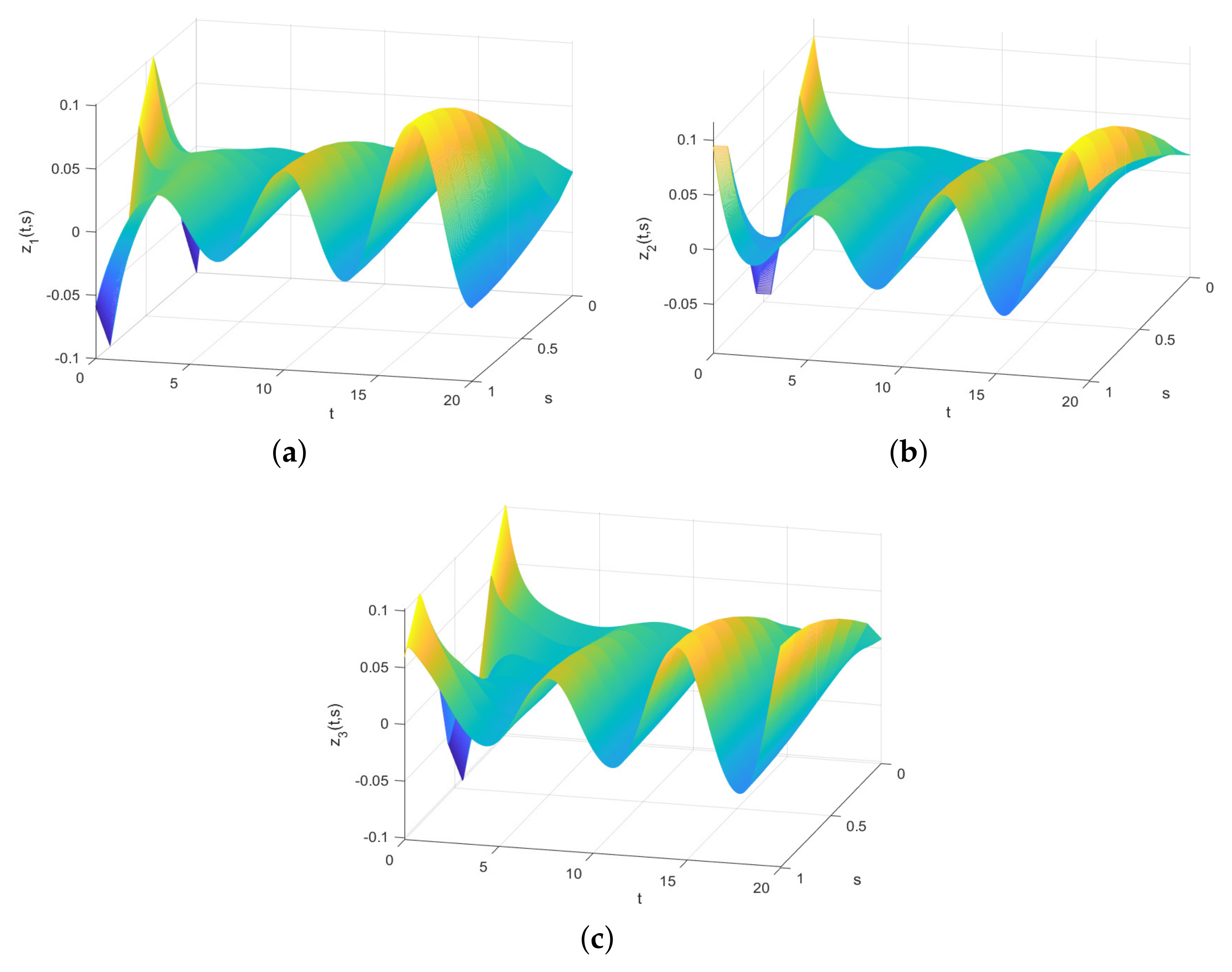
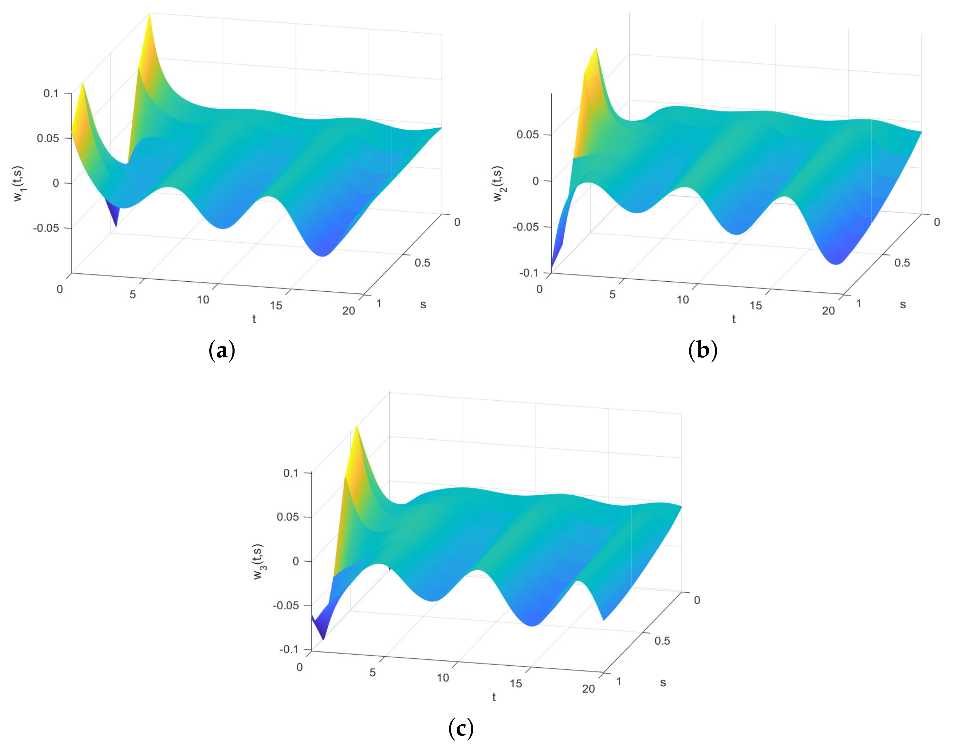
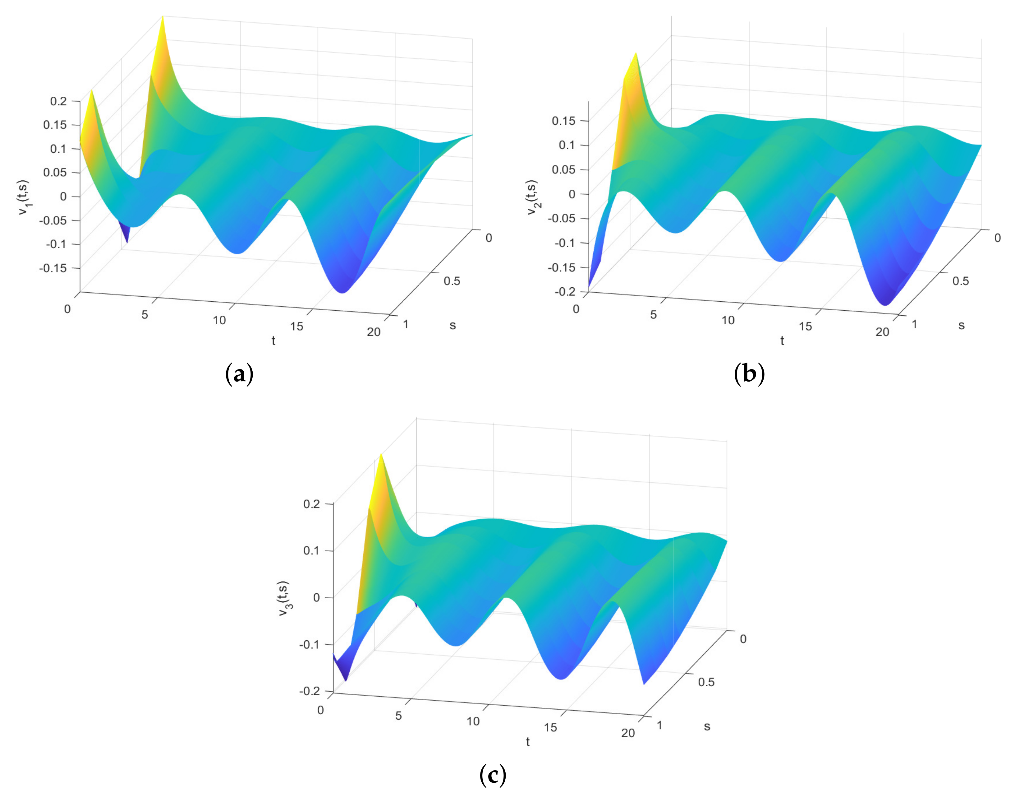
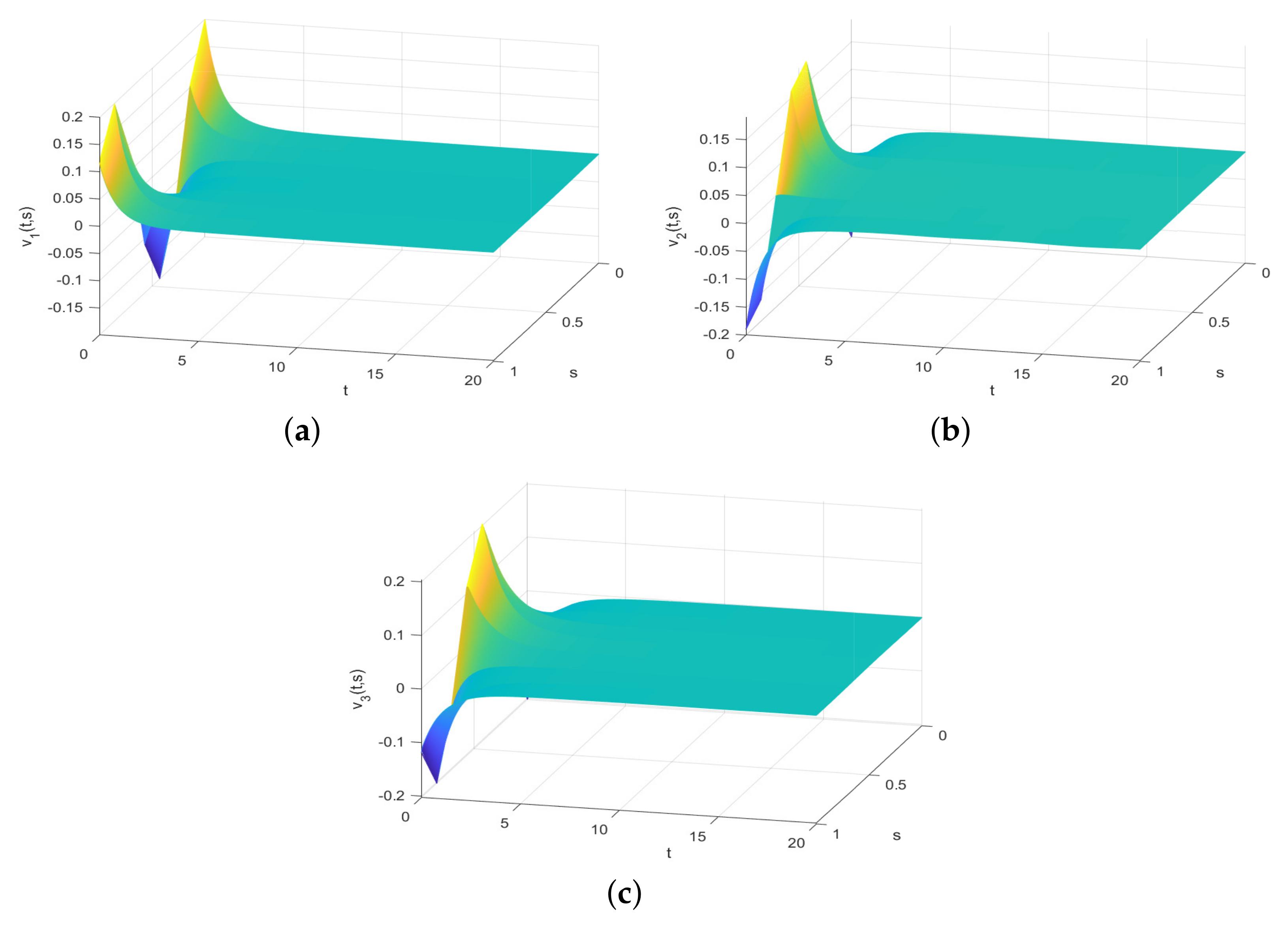
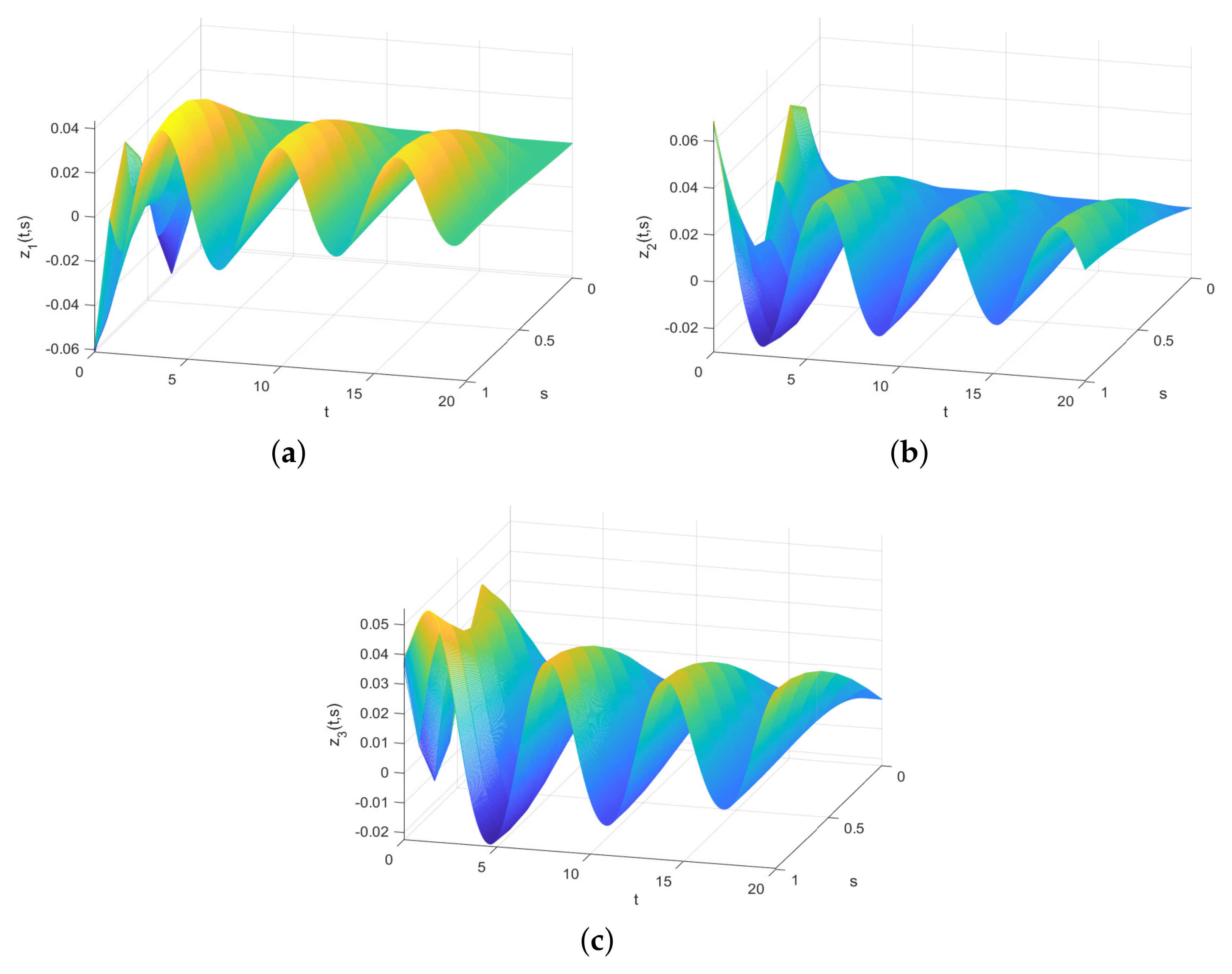
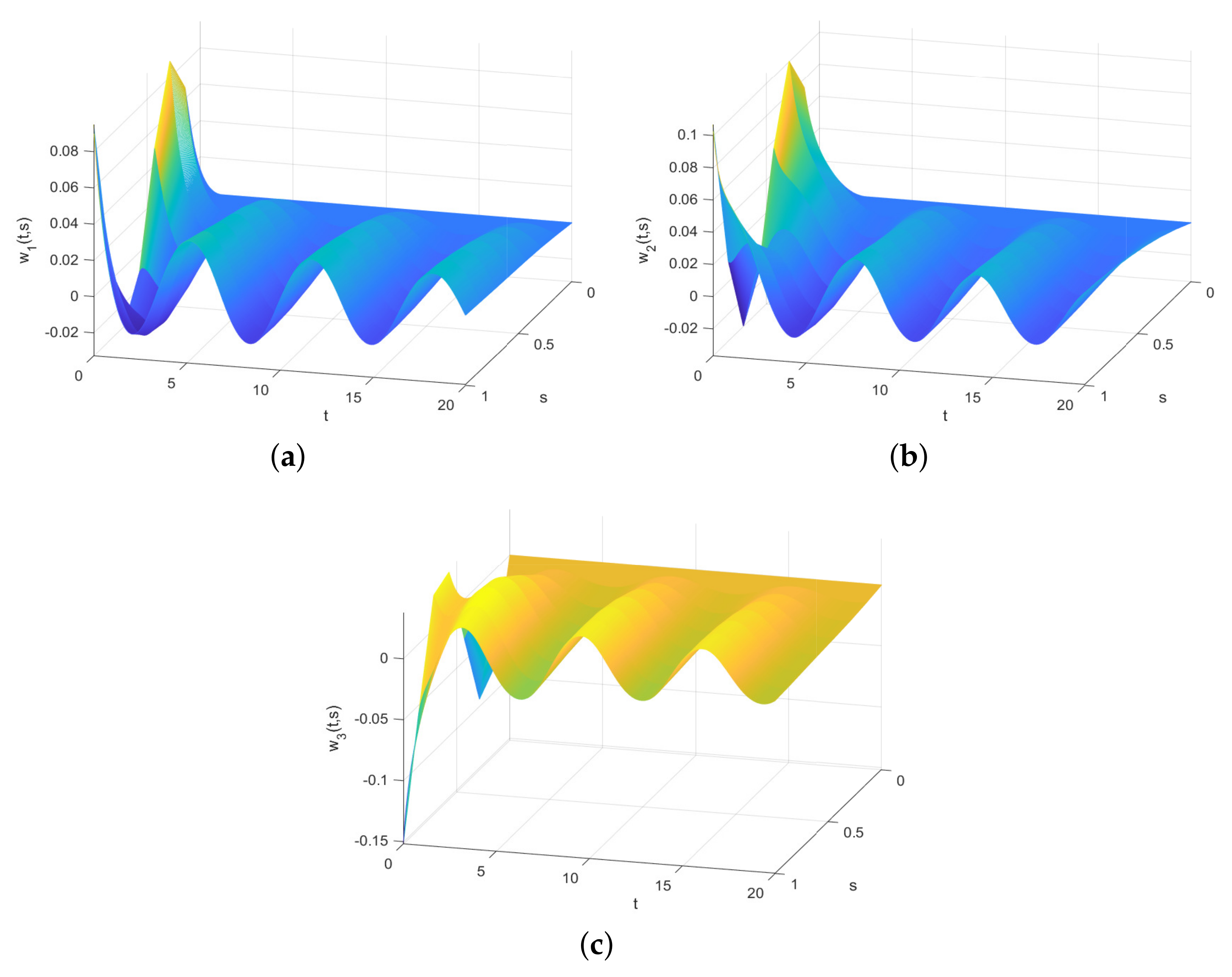
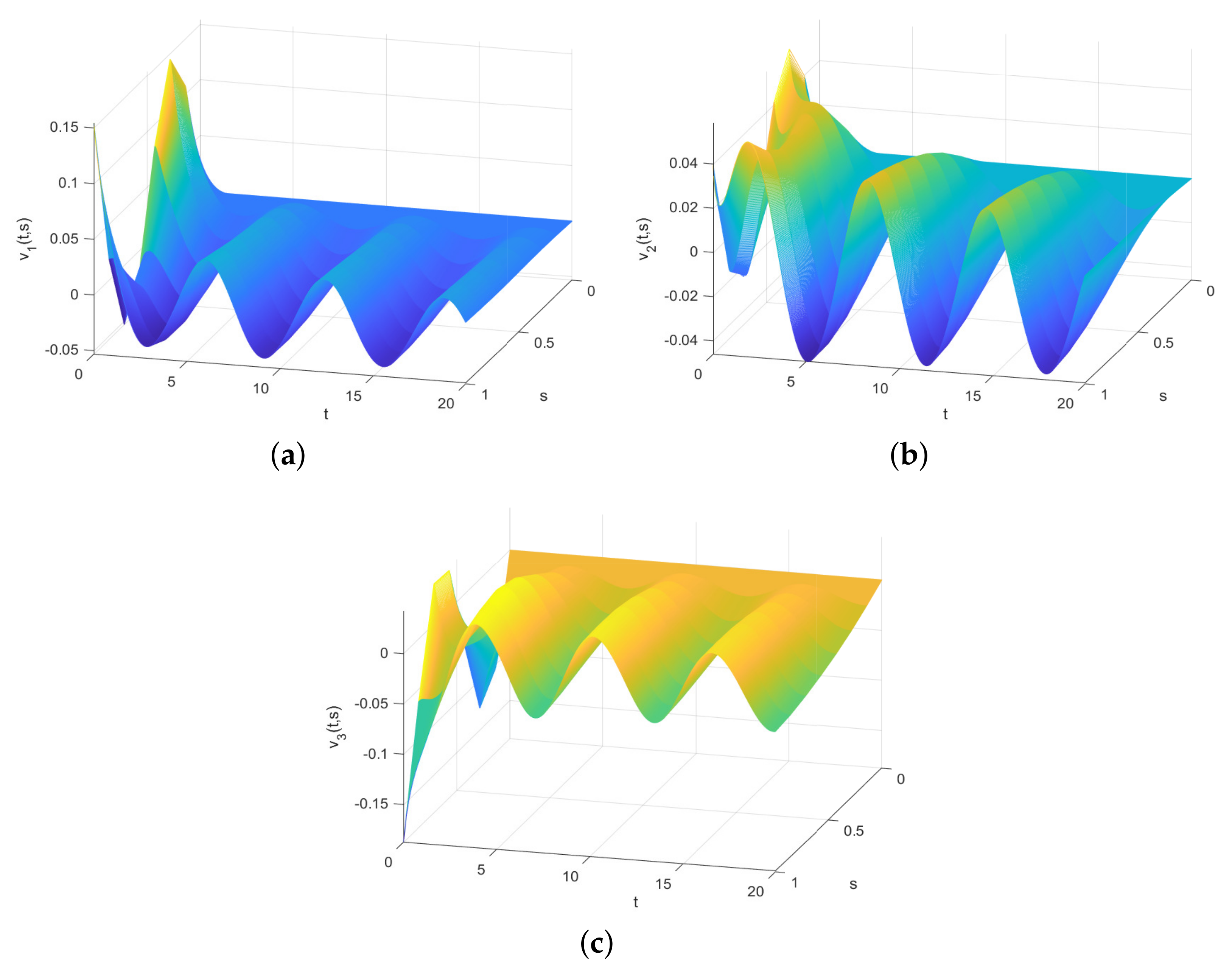
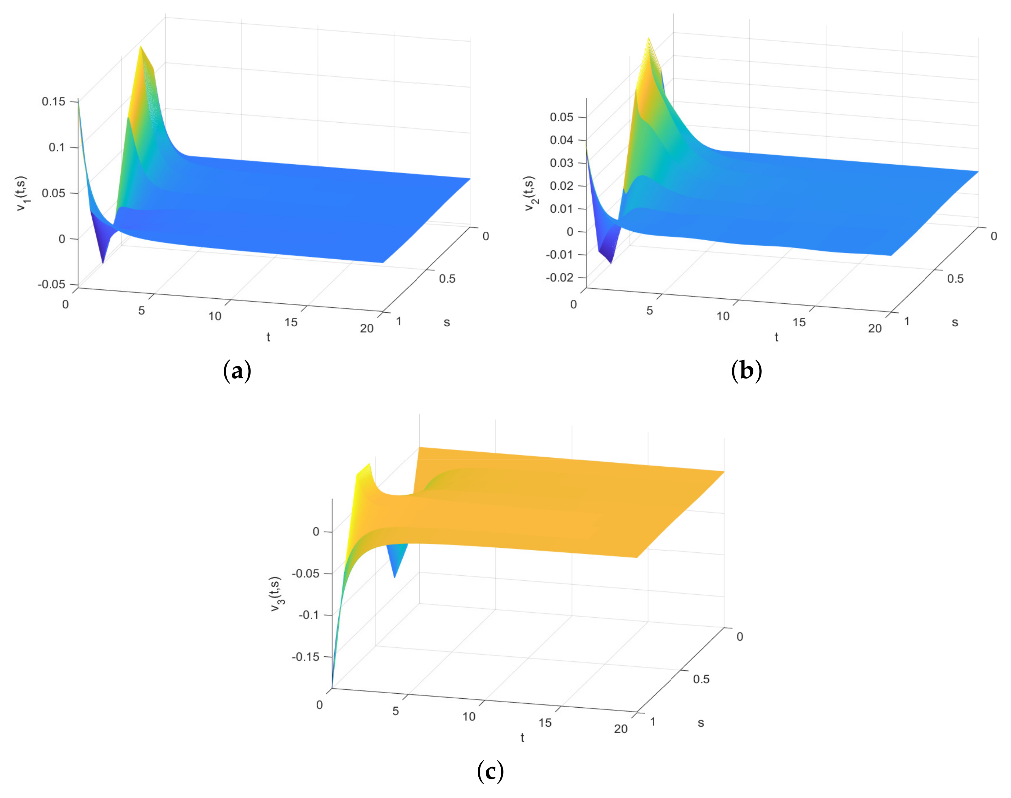
4. Numerical Simulations

In this part, the validity of the theoretical results under Neumann boundary conditions (13) and (14) and mixed boundary conditions (43) and (44) is verified via two numerical examples.

Example 1.

Consider system (1) with Neumann boundary condition (3), and let $n=3$. The specific parameters of system (1) are as follows: $\beta =0.95,k_i=1.5,d_i=0.5,{\overline{d}}_i=0.4,a_i=1,T_{ij}=Q_{ij}=H_{ij}=1,{\chi }_i=0.8,f_j\left(z_j(t,s)\right)=0.5(|z_j(t,s)+1|-|z_j(t,s)-1|),i,j\in \mathcal{I}=\{1,2,3\},$

$$\begin{array}{c}\hfill B=\left(\begin{array}{ccc}1.36& -1.35& 1.35\\ 1.42& 1.27& -1.31\\ -1.42& 1.39& 1.64\end{array}\right),\xi =\left(\begin{array}{ccc}0.2& 0.5& 0.3\\ 0.5& 0.2& 0.4\\ 0.3& 0.4& 0.3\end{array}\right),\eta =\left(\begin{array}{ccc}0.5& 0.3& 0.2\\ 0.3& 0.4& 0.2\\ 0.5& 0.5& 0.3\end{array}\right).\end{array}$$

The initial values of system (1) are $z_1(0,s)=-0.1\left(\cos \left(2.3\pi s\right)\right), z_2(0,s)=0.1\left(\cos \left(2.1\pi s\right)\right), z_3(0,s)=0.1\left(\cos \left(2.3\pi s\right)\right), {\partial }_t^{\beta }{z}_1(0,s)=-0.1(-\cos \left(2.3\pi s\right)), {\partial }_t^{\beta }{z}_2(0,s)=-0.1\cos \left(2.1\pi s\right), {\partial }_t^{\beta }{z}_3(0,s)=0.1\cos \left(2.3\pi s\right).$

For the response system (4) with Neumann boundary condition (6), the initial values are $w_1(0,s)=0.1\left(\cos \left(2.3\pi s\right)\right), w_2(0,s)=-0.1\left(\cos \left(2.1\pi s\right)\right), w_3(0,s)=-0.1\left(\cos \left(2.3\pi s\right)\right), {\partial }_t^{\beta }{w}_1(0,s)=-0.1\left(\cos \left(2.3\pi s\right)\right), {\partial }_t^{\beta }{w}_2(0,s)=0.1\left(\cos \left(2.1\pi s\right)\right), {\partial }_t^{\beta }{w}_3(0,s)=-0.1\left(\cos \left(2.2\pi s\right)\right).$ Other parameters are the same as those of system (1).

By using the LMI box in MATLAB, we can determine P = diag{−4.28,−4.28,−4.28} satisfying (16) and select the appropriate parameters $\epsilon =1.18,l=1,{\theta }_i=1,i=1,2,3$. Through simple calculations, the conditions of Theorem 1 are met. Next, the corresponding MATLAB R2024a simulations are demonstrated in Figure 1, Figure 2, Figure 3 and Figure 4. The state trajectories of systems (1) and (4) are revealed in Figure 1 and Figure 2. The trajectories of error system (7) without the controller and with the controller are shown in Figure 3 and Figure 4. It follows from Figure 3 and Figure 4 that, under controller (15), systems (1) and (4) with Neumann boundary conditions (13) and (14) are global Mittag-Leffler synchronized.

Remark 7.

As shown in Figure 1, Figure 2, Figure 3 and Figure 4, the simulations confirm the theoretical results. In fact, boundary synchronization control in FOFRDINNs has a broad array of practical applications, particularly in areas such as image encryption, signal processing and UAV formation flight control. Taking the military reconnaissance application scenario as an example, the efficient and stable flight of a UAV formation can be realized by reasonably configuring the boundary conditions and control parameters.

Example 2.

Consider system (1) with mixed boundary condition (43), where $n=3$, $\beta =0.9$, $k_1=1.2$, $k_2=1.3$, $k_3=1.5$, $d_i=0.5$, $\overline{d_i}=0.4$, $a_i=1$, $T_{ij}=Q_{ij}=H_{ij}=1.3$, ${\chi }_i=1.2$, $f_j\left(z_j(t,s)\right)=\tanh \left(z_j(t,s)\right)$, $i,j\in \mathcal{I}=\{1,2,3\},$

$$\begin{array}{c}\hfill B=\left(\begin{array}{ccc}1.41& -1.38& 1.57\\ 1.31& 1.67& -1.43\\ -1.42& 1.69& 1.59\end{array}\right),\xi =\left(\begin{array}{ccc}0.8& 0.6& 0.3\\ 0.5& 0.2& 0.4\\ 0.3& 0.3& 0.6\end{array}\right),\eta =\left(\begin{array}{ccc}0.5& 0.3& 0.3\\ 0.3& 0.4& 0.2\\ 0.5& 0.5& 0.4\end{array}\right).\end{array}$$

The initial values of (1) are set as $z_1(0,s)=-0.05(s^2+\sin \left(2.1\pi s\right)), z_2(0,s)=0.04(s^2+\sin \left(2.3\pi s\right)), z_3(0,s)=0.03(s^2+\sin \left(2.1\pi s\right)), {\partial }_t^{\beta }{z}_1(0,s)=-0.08(s+\sin \left(2.1\pi s\right)), {\partial }_t^{\beta }{z}_2(0,s)=0.06(s+\sin \left(2.1\pi s\right)), {\partial }_t^{\beta }{z}_3(0,s)=-0.09(s+\sin \left(2.2\pi s\right)).$

For the response system (4) with mixed boundary condition (44), the initial values are as follows: $w_1(0,s)=0.08(s^2+\sin \left(2.1\pi s\right)), w_2(0,s)=0.09(s^2+\sin \left(2.1\pi s\right)), w_3(0,s)=-0.09(s^2+\sin \left(2.3\pi s\right)), {\partial }_t^{\beta }{w}_1(0,s)=-0.06(s+\sin \left(2.2\pi s\right)), {\partial }_t^{\beta }{z}_2(0,s)=-0.05(s+\sin \left(2.2\pi s\right)), {\partial }_t^{\beta }{w}_3(0,s)=0.07(s+\sin \left(2.4\pi s\right)).$ Other parameters are the same as those of system (1).

Analogously, applying MATLAB, one can find $P=\mathrm{diag}\{-4.8,-4.8,-4.8\}$ and choose $\epsilon =0.72,l=1,{\theta }_i=1,i=1,2,3.$ By simple computation, the conditions of Theorem 2 are satisfied. Subsequently, the corresponding MATLAB R2024a simulations are demonstrated in Figure 5, Figure 6, Figure 7 and Figure 8. The state trajectories of systems (1) and (4) are revealed in Figure 7 and Figure 8. The trajectories of error system (7) without the controller and with the controller are shown in Figure 7 and Figure 8. From Figure 7 and Figure 8, it can be seen that, under controller (15), systems (1) and (4) with mixed boundary conditions (43) and (44) can reach global Mittag-Leffler synchronization.

5. Conclusions

In this paper, boundary control is employed to research the synchronization problem of FOFRDINNs. A class of generalized fractional-order NNs i.e., FOFRDINNs are established, which concurrently integrate fuzzy logic, inertial terms and reaction–diffusion terms. This integrated framework effectively handles renewable power fluctuation uncertainties, characterizes robotic joint dynamics and models spatial transmission processes in smart grids, thereby significantly enhancing its fidelity in practical engineering systems. In order to reduce the waste of resources, a boundary controller is designed to address the synchronization issue of FOFRDINNs. At the same time, based on the non-reduced-order method, the corresponding synchronization criteria are obtained under three boundary conditions. Finally, two numerical examples are provided to demonstrate the effectiveness of the boundary controller.

Time-varying delays are common in practical systems, which may lead to the performance degradation or even instability of the controller designed in this paper. Moreover, considering that the internal information state cannot be directly measured, introducing observation control is necessary. Thus, our future work is to study the synchronization behavior of FOFRDINNs with time-varying delays by utilizing observation control.

References

1. Chen, C.; Wu, Y.; Dai, Q.; Zhou, H.Y.; Xu, M.; Yang, S.; Han, X.; Yu, Y. A survey on graph neural networks and graph transformers in computer vision: A task-oriented perspective. IEEE Trans. Pattern Anal. Mach. Intell. 2024, 46, 10297–10318. [Google Scholar] [CrossRef] [PubMed]
2. Du, J.; Bai, Y.; Li, Y.; Geng, J.; Huang, Y.; Chen, H. Evolutionary end-to-end autonomous driving model with continuous-time neural networks. IEEE/ASME Trans. Mechatron. 2024, 29, 2983–2990. [Google Scholar] [CrossRef]
3. Shi, J.; Chen, T.; Lai, W.; Zhang, S.; Li, X. Pretrained quantum-inspired deep neural network for natural language processing. IEEE Trans. Cybern. 2024, 54, 5973–5985. [Google Scholar] [CrossRef] [PubMed]
4. Bi, X.A.; Chen, K.; Jiang, S.; Luo, S.; Zhou, W.; Xing, Z.; Xu, L.; Liu, Z.; Liu, T. Community graph convolution neural network for alzheimer’s disease classification and pathogenetic factors identification. IEEE Trans. Neural Netw. Learn. Syst. 2025, 36, 1959–1973. [Google Scholar] [CrossRef]
5. Li, P.; Gao, R.; Xu, C.; Li, Y.; Akgül, A.; Baleanu, D. Dynamics exploration for a fractional-order delayed zooplankton–phytoplankton system. Chaos Solitons Fractals 2023, 166, 112975. [Google Scholar] [CrossRef]
6. Xua, C.; Liaob, M.; Farman, M.; Shehzade, A. Hydrogenolysis of glycerol by heterogeneous catalysis: A fractional order kinetic model with analysis. MATCH Commun. Math. Comput. Chem. 2024, 91, 635–664. [Google Scholar] [CrossRef]
7. Yang, S.; Hu, C.; Yu, J.; Jiang, H. Exponential stability of fractional-order impulsive control systems with applications in synchronization. IEEE Trans. Cybern. 2020, 50, 3157–3168. [Google Scholar] [CrossRef]
8. Cao, S.; Chen, Y. Data-driven controllability and controller designs for nabla fractional order systems. IEEE Control Syst. Lett. 2024, 8, 3033–3038. [Google Scholar] [CrossRef]
9. Yan, Y.; Zhang, H.; Mu, Y.; Sun, J. Fault-tolerant fuzzy-resilient control for fractional-order stochastic underactuated system with unmodeled dynamics and actuator saturation. IEEE Trans. Cybern. 2023, 54, 988–998. [Google Scholar] [CrossRef]
10. Cao, B.; Nie, X.; Zheng, W.X.; Cao, J. Multistability of state-dependent switched fractional-order hopfield neural networks with mexican-hat activation function and its application in associative memories. IEEE Trans. Neural Netw. Learn. Syst. 2025, 36, 1213–1227. [Google Scholar] [CrossRef]
11. Arena, P.; Fortuna, L.; Porto, D. Chaotic behavior in noninteger-order cellular neural networks. Phys. Rev. E 2000, 61, 776. [Google Scholar] [CrossRef] [PubMed]
12. Wei, C.; Wang, X.; Hui, M.; Zeng, Z. Quasi-synchronization of fractional multiweighted coupled neural networks via aperiodic intermittent control. IEEE Trans. Cybern. 2024, 54, 1671–1684. [Google Scholar] [CrossRef] [PubMed]
13. Kao, Y.; Wang, C.; Xia, H.; Cao, Y. Projective synchronization for uncertain fractional reaction-diffusion systems via adaptive sliding mode control based on finite-time scheme. In Analysis and Control for Fractional-Order Systems; Springer: Berlin/Heidelberg, Germany, 2024; pp. 141–163. [Google Scholar]
14. Li, H.L.; Cao, J.; Hu, C.; Jiang, H.; Alsaadi, F.E. Synchronization analysis of discrete-time fractional-order quaternion-valued uncertain neural networks. IEEE Trans. Neural Netw. Learn. Syst. 2024, 35, 14178–14189. [Google Scholar] [CrossRef] [PubMed]
15. Zhang, R.; Qiu, K.; Liu, C.; Ma, H.; Chu, Z. Comparison principle based synchronization analysis of fractional-order chaotic neural networks with multi-order and its circuit implementation. Fractal Fract. 2025, 9, 273. [Google Scholar] [CrossRef]
16. Yan, W.; Jiang, Z.; Huang, X.; Ding, Q. Adaptive neural network synchronization control for uncertain fractional-order time-delay chaotic systems. Fractal Fract. 2023, 7, 288. [Google Scholar] [CrossRef]
17. Maharajan, C.; Sowmiya, C.; Xu, C. Lagrange stability of inertial type neural networks: A Lyapunov-Krasovskii functional approach. Evol. Syst. 2025, 16, 63. [Google Scholar] [CrossRef]
18. Ullah, A.; Ullah, A.; Ahmad, S.; Van Hoa, N. Fuzzy Yang transform for second order fuzzy differential equations of integer and fractional order. Phys. Scr. 2023, 98, 044003. [Google Scholar] [CrossRef]
19. Babcock, K.; Westervelt, R. Stability and dynamics of simple electronic neural networks with added inertia. Phys. D Nonlinear Phenom. 1986, 23, 464–469. [Google Scholar] [CrossRef]
20. Liu, X.; He, H.; Cao, J. Event-triggered bipartite synchronization of delayed inertial memristive neural networks with unknown disturbances. IEEE Trans. Control Netw. Syst. 2024, 11, 1408–1419. [Google Scholar] [CrossRef]
21. Zhang, Z.; Wang, S.; Wang, X.; Wang, Z.; Lin, C. Event-triggered synchronization for delayed quaternion-valued inertial fuzzy neural networks via nonreduced order approach. IEEE Trans. Fuzzy Syst. 2023, 31, 3000–3014. [Google Scholar] [CrossRef]
22. Li, L.; Cui, Q.; Cao, J.; Qiu, J.; Sun, Y. Exponential synchronization of coupled inertial neural networks with hybrid delays and stochastic impulses. IEEE Trans. Neural Netw. Learn. Syst. 2024, 535, 15402–15414. [Google Scholar] [CrossRef] [PubMed]
23. Cheng, Y.; Zhang, H.; Zhang, W.; Zhang, H. Novel algebraic criteria on global Mittag–Leffler synchronization for FOINNs with the Caputo derivative and delay. J. Appl. Math. Comput. 2022, 68, 3527–3544. [Google Scholar] [CrossRef]
24. Luo, L.; Li, L.; Huang, W.; Cui, Q. Stability of the Caputo fractional-order inertial neural network with delay-dependent impulses. Neurocomputing 2023, 520, 25–32. [Google Scholar] [CrossRef]
25. Li, Z.; Zhang, Y. The boundedness and the global mittag-leffler synchronization of fractional-order inertial Cohen–Grossberg neural networks with time delays. Neural Process. Lett. 2022, 54, 597–611. [Google Scholar] [CrossRef]
26. Ullah, A.; Ullah, A.; Ahmad, S.; Ahmad, I.; Akgül, A. On solutions of fuzzy fractional order complex population dynamical model. Numer. Methods Partial Differ. Equ. 2023, 39, 4595–4615. [Google Scholar] [CrossRef]
27. Wan, P.; Zeng, Z. Stability and stabilization of Takagi–Sugeno fuzzy second-fractional-order linear networks via nonreduced-order approach. IEEE Trans. Syst. Man Cybern. Syst. 2022, 52, 6524–6533. [Google Scholar] [CrossRef]
28. Peng, Q.; Jian, J. Asymptotic synchronization of second-fractional-order fuzzy neural networks with impulsive effects. Chaos Solitons Fractals 2023, 168, 113150. [Google Scholar] [CrossRef]
29. Cui, Q.; Xu, C.; Xu, Y.; Ou, W.; Pang, Y.; Liu, Z.; Shen, J.; Baber, M.Z.; Maharajan, C.; Ghosh, U. Bifurcation and Controller design of 5D BAM neural networks with time delay. Int. J. Numer. Model. Electron. Netw. Devices Fields 2024, 37, e3316. [Google Scholar] [CrossRef]
30. Maharajan, C.; Sowmiya, C.; Xu, C. Delay dependent complex-valued bidirectional associative memory neural networks with stochastic and impulsive effects: An exponential stability approach. Kybernetika 2024, 60, 317–356. [Google Scholar] [CrossRef]
31. Hao, R.; Yang, Y.; Liu, F.; Zhou, B. Stability and bipartite synchronization of fractional-order coupled reaction–diffusion neural networks under unbalanced graph. Chaos Solitons Fractals 2024, 189, 115583. [Google Scholar] [CrossRef]
32. Ma, L.; Tang, D. Dynamical behavior of a three-species diffusion-advection predator-prey-mutualist model in heterogeneous environments. J. Differ. Equ. 2025, 424, 330–380. [Google Scholar] [CrossRef]
33. Jiao, X.; Liu, L.; Yu, X. Rich dynamics of a reaction–diffusion Filippov Leslie–Gower predator–prey model with time delay and discontinuous harvesting. Math. Comput. Simul. 2025, 228, 339–361. [Google Scholar] [CrossRef]
34. Xu, Y.; Jiang, Z.; Xie, X.; Li, W.; Wu, Y. Fuzzy-based bipartite quasi-synchronization of fractional-order heterogeneous reaction-diffusion neural networks via intermittent control. IEEE Trans. Circuits Syst. I Regul. Pap. 2024, 71, 3880–3890. [Google Scholar] [CrossRef]
35. Wang, J.L. Passivity for multiadaptive coupled fractional-order reaction-diffusion neural networks. In Dynamical Behaviors of Fractional-Order Complex Dynamical Networks; Springer: Berlin/Heidelberg, Germany, 2024; pp. 141–168. [Google Scholar]
36. Wang, H.; Gu, Y.; Zhang, X.; Yu, Y. Stability and synchronization of fractional-order reaction–diffusion inertial time-delayed neural networks with parameters perturbation. Neural Netw. 2024, 179, 106564. [Google Scholar] [CrossRef]
37. Langlands, T.; Henry, B.; Wearne, S. Fractional cable equation models for anomalous electrodiffusion in nerve cells: Infinite domain solutions. J. Math. Biol. 2011, 59, 761–808. [Google Scholar] [CrossRef]
38. Tzou, D.Y. A unified field approach for heat conduction from macro-to micro-scales. J. Heat Transf. 1995, 117, 8–16. [Google Scholar] [CrossRef]
39. Greenberg, J.M.; Tsien, L.T. The effect of boundary damping for the quasilinear wave equation. J. Differ. Equ. 1984, 52, 66–75. [Google Scholar] [CrossRef]
40. Shi, T.; Hu, C.; Yu, J.; Zhu, Q.; Huang, T. Internal/Boundary control-based fixed-time synchronization for spatiotemporal networks. IEEE Trans. Cybern. 2024, 54, 6693–6706. [Google Scholar] [CrossRef]
41. Liu, X.Z.; Wu, K.N.; Ahn, C.K. Intermittent boundary control for synchronization of fractional delay neural networks with diffusion terms. IEEE Trans. Syst. Man Cybern. Syst. 2023, 53, 2900–2912. [Google Scholar] [CrossRef]
42. Sun, Y.; Hu, C.; Yu, J.; Shi, T. Synchronization of fractional-order reaction-diffusion neural networks via mixed boundary control. Appl. Math. Comput. 2024, 450, 127982. [Google Scholar] [CrossRef]
43. Wang, Z.P.; Zhang, X.; Qiao, J.F.; Wu, H.N.; Huang, T. Synchronization of reaction-diffusion neural networks with random time-varying delay via intermittent boundary control. Neurocomputing 2023, 556, 126645. [Google Scholar] [CrossRef]
44. Podlubny, I. Fractional Differential Equations: An Introduction to Fractional Derivatives, Fractional Differential Equations, to Methods of Their Solution and Some of Their Applications; Elsevier: Amsterdam, The Netherlands, 1999; Volume 198. [Google Scholar]
45. Miller, K.S.; Ross, B. An Introduction to the Fractional Calculus and Fractional Differential Equations; Wiley: Hoboken, NJ, USA, 1993. [Google Scholar]
46. Yang, T.; Yang, L.B. The global stability of fuzzy cellular neural network. IEEE Trans. Circuits Syst. I Fundam. Theory Appl. 1996, 43, 880–883. [Google Scholar] [CrossRef]
47. Chen, J.; Zeng, Z.; Jiang, P. Global Mittag-Leffler stability and synchronization of memristor-based fractional-order neural networks. Neural Netw. 2014, 51, 1–8. [Google Scholar] [CrossRef] [PubMed]
48. Wang, Z.; Zhang, W.; Zhang, H.; Chen, D.; Cao, J.; Abdel-Aty, M. Finite-time quasi-projective synchronization of fractional-order reaction-diffusion delayed neural networks. Inf. Sci. 2025, 686, 121365. [Google Scholar] [CrossRef]
Figure 1. The trajectories of z i ( t ) : (a) z 1 ( t ) ; (b) z 2 ( t ) ; (c) z 3 ( t ) .
Fractalfract 09 00405 g001
Figure 2. The trajectories of w i ( t ) : (a) w 1 ( t ) ; (b) w 2 ( t ) ; (c) w 3 ( t ) .
Fractalfract 09 00405 g002
Figure 3. The trajectories of v i ( t ) without control: (a) v 1 ( t ) ; (b) v 2 ( t ) ; (c) v 3 ( t ) .
Fractalfract 09 00405 g003
Figure 4. The trajectories of v i ( t ) with control: (a) v 1 ( t ) ; (b) v 2 ( t ) ; (c) v 3 ( t ) .
Fractalfract 09 00405 g004
Figure 5. The trajectories of z i ( t ) : (a) z 1 ( t ) ; (b) z 2 ( t ) ; (c) z 3 ( t ) .
Fractalfract 09 00405 g005
Figure 6. The trajectories of w i ( t ) : (a) w 1 ( t ) ; (b) w 2 ( t ) ; (c) w 3 ( t ) .
Fractalfract 09 00405 g006
Figure 7. The trajectories of v i ( t ) without control: (a) v 1 ( t ) ; (b) v 2 ( t ) ; (c) v 3 ( t ) .
Fractalfract 09 00405 g007
Figure 8. The trajectories of v i ( t ) with control: (a) v 1 ( t ) ; (b) v 2 ( t ) ; (c) v 3 ( t ) .
Fractalfract 09 00405 g008
Disclaimer/Publisher’s Note: The statements, opinions and data contained in all publications are solely those of the individual author(s) and contributor(s) and not of MDPI and/or the editor(s). MDPI and/or the editor(s) disclaim responsibility for any injury to people or property resulting from any ideas, methods, instructions or products referred to in the content.