Spatiotemporal Analysis of Disease Spread Using a Soliton-Based SIR Framework for Nomadic Populations

Abstract

This study enhances the classical deterministic SIR model by incorporating soliton-like dynamics and gradient-induced diffusion, effectively capturing the complex spatiotemporal patterns of disease transmission within nomadic populations. The proposed model incorporates an advection–diffusion mechanism that modulates the spatial gradients in infection dynamics, transitioning from highly localized infection peaks to distributed infection fronts. We discussed the role of diffusion coefficients in shaping the spatial distribution of susceptible, infected, and recovered populations, as well as the impact of gradient-induced advection in mitigating epidemic intensity. Numerical simulations demonstrate the effects of varying key parameters such as transmission rates, recovery rates, and advection–diffusion coefficients on the epidemic’s progression. The soliton-like dynamics ensure the stability of infection waves over time, specifying targeted intervention strategies such as localized quarantines and vaccination campaigns. This model underscores the critical importance of spatial heterogeneity and mobility patterns in managing infectious diseases. The applicability of the model has been tested using the AIDS data from the last 25 years.

1. Introduction

The study of nonlinear dynamics in complex systems has emerged as a profound and multifaceted field that spans a diverse range of disciplines, including physics, biology, epidemiology, and engineering. At the heart of this exploration lies the intricate interplay between nonlinearity, dissipation, and dispersion mechanisms that together give rise to phenomena such as wave propagation, pattern formation, and, notably, solitons. Solitons, first discovered in the context of shallow-water waves by John Scott Russell in the 19th century, represent a class of solutions to certain nonlinear partial differential equations (PDEs) that exhibit remarkable stability and persistence. Unlike ordinary waves, solitons maintain their shape and speed even after interactions, making them a quintessential feature in a variety of natural and engineered systems [1]. The authors suggested that the nervous macroscopic activity of the central nervous system could be assessed in terms of solitons [2]. Soliton theory also finds natural applications in the modeling of spatial systems, where interactions between localized disturbances propagate without spreading. This characteristic is of particular importance in systems that exhibit a balance between nonlinear and dispersive effects, such as optical fibers, where solitons enable the transmission of information over long distances without degradation. In the biological realm, solitons have been proposed as mechanisms for signal transmission in nerve fibers, whereas in plasma physics, they describe coherent structures that emerge in the context of magnetic confinement in fusion devices.

Mathematical modeling plays an essential role in understanding the transmission of epidemic diseases and predicting the effectiveness of new control strategies [3,4,5,6]. These models strike a balance between accurately representing the biological progression of infections and ensuring robust connections to real-world data. Models have been developed on multiple scales, from localized outbreaks to larger population-wide studies, providing estimates for key threshold parameters. Environmental factors remain crucial in shaping biological processes and real-world systems. Recent advances in surrogate modeling and multisource information fusion have demonstrated the effectiveness of kernel-based methods [7,8]. Recent research reveals causal links between HbA1c and diseases and analyzes healthcare travel burdens [9].

Variations in environmental conditions and randomness introduce significant unpredictability in the spread of epidemics, making future outcomes highly uncertain [10,11,12]. Thus, environmental fluctuations and demographic diversity can greatly influence the dynamics of infectious disease transmission. Beyond the realm of pure solitons, the notion of “soliton-like” phenomena has been used to describe systems in which solitary wave behavior is observed, albeit under more general conditions [3]. In these systems, nonlinearities may be balanced not solely by dispersion but also by gradient effects, dissipation, or other forms of stabilization [13,14]. This generalization broadens the applicability of soliton theory to complex systems where exact soliton solutions may not exist, but the underlying dynamics retain the essential features of localized wave packets that propagate stably through the medium [15,16]. In this study, we propose a novel extension of the classical Susceptible-Infected-Recovered (SIR) model by embedding soliton-like behavior into the infected population dynamics, along with spatial gradient terms. The rationale for this extension stems from the necessity to encapsulate the complex spatiotemporal dynamics that are observed in real-world disease transmission. The proposed model amalgamates spatial diffusion and soliton propagation, yielding a system that more accurately captures the localized spread of infection within heterogeneous populations. This hybrid dynamical system, to the best of our knowledge, represents an innovative approach in epidemiological modeling and has yet to be explored in the current literature. The soliton-like dynamics incorporated into the infected compartment enable the precise identification of regions exhibiting high infection concentrations, which are interpreted as “infection hotspots.” These concentrated areas exhibit characteristics analogous to soliton wave packets, which are highly stable and capable of maintaining their structure over time and space. Given the heterogeneous nature of urban populations, characterized by varying mobility patterns and density distributions, the soliton model provides a powerful tool for predicting and controlling the disease spread across different neighborhoods.

The motivation for this work stems from the need to model and understand the spread of infectious diseases in populations that exhibit significant spatial mobility, such as nomadic and semi-nomadic groups [17,18,19,20]. These populations, often living in rural or semi-rural environments, migrate seasonally with their livestock, increasing their exposure to zoonotic disease pathogens that are transmitted between animals and humans. Examples include brucellosis, anthrax, and Rift Valley fever, all of which are highly prevalent in such communities. These diseases are of particular concern because they can spread not only through human contact but also through interactions with infected animals such as goats, sheep, and cattle. Traditional epidemiological models often fail to account for the complex spatial and temporal dynamics inherent in such mobile populations, where individuals are exposed to different environmental conditions and vectors over time. The novelty of this work lies in the introduction of a spatial SIR model that incorporates gradient-induced advection and diffusion terms to simulate the spatiotemporal spread of diseases in populations that experience constant movement across space [21,22]. The gradient-induced advection mechanism models the movement of individuals in response to infection gradients, a phenomenon particularly relevant to nomadic populations that often move in response to environmental conditions and herd health. The diffusion term captures the random movement of individuals and infected animals across space, effectively modeling the spatial heterogeneity observed in these communities.

2. Problem Formulation

The following assumptions are made in the epidemic model with spatial diffusion:

•

Individuals in the population mix homogeneously, meaning the contact rate between susceptible and infected individuals is proportional to their densities.

•

The total population remains constant. Individuals transition between susceptible, infected, and recovered classes, but no individuals enter or leave the population.

•

The model excludes natality dynamics, given their negligible impact on short-term epidemic progression and disease transmission.

•

The term $-B{I}^3$ in the infected equation represents saturation or nonlinear feedback, reducing transmission at high infection levels.

•

The diffusion coefficients $D_S$, $D_I$, $D_R$ are strictly positive real-valued constants, representing the rates of random spatial movement for the susceptible, infected, and recovered populations, respectively. The gradient variable related to advection A is also a real-valued parameter and can take positive or negative values depending on the direction of movement relative to the infection gradients.

•

The model operates on a finite spatial domain with no external migration.

Consider the epidemic model with spatial diffusion,

$$\begin{array}{cc}\hfill {\displaystyle \frac{dS}{dt}}& =-\beta SI-\mu S+D_S{\nabla }^{2}S,\hfill \\ \hfill {\displaystyle \frac{dI}{dt}}& =\beta SI-(\gamma +\alpha )I-B{I}^3+D_I{\nabla }^{2}I+A\nabla I,\hfill \\ \hfill {\displaystyle \frac{dR}{dt}}& =\gamma I-\nu R+D_R{\nabla }^{2}R,\hfill \end{array}$$

(1)

with boundary conditions

$${\displaystyle \frac{\partial S}{\partial n}}=0,{\displaystyle \frac{\partial I}{\partial n}}=0,{\displaystyle \frac{\partial R}{\partial n}}=0,\mathrm{for}x\in \partial \mathsf{\Omega },t>0.$$

(2)

Table 1. Parameter definitions for the epidemic model.

Parameter	Definition
$\beta$	Transmission rate.
$\mu$	Death rate.
$\gamma$	Recovery rate.
$\alpha$	Additional damping rate for infected individuals (enhanced recovery).
$\nu$	Loss of immunity.
$D_S$	Diffusion coefficient for susceptible individuals.
$D_I$	Diffusion coefficient for infected individuals.
$D_R$	Diffusion coefficient for recovered individuals.
A	Advection coefficient for the movement of infected individuals.
B	Saturation parameter reducing transmission at high infection levels.
∇	Laplacian operator.
$S(x,t)$	Susceptible population density at position x and time t.
$I(x,t)$	Infected population density at position x and time t.
$R(x,t)$	Recovered population density at position x and time t.

presents the parameter explanations and values.

3. Theoretical Analysis

Theorem 1.

Let $\mathsf{\Omega }\subset {\mathbb{R}}^n$ be a bounded domain with smooth boundary $\partial \mathsf{\Omega }$, and let $T>0$ be a fixed final time. Assume that the following conditions hold:

•

$S_0,I_0,R_0\in H^1\left(\mathsf{\Omega }\right)$;

•

$S_0\left(x\right)\ge 0$, $I_0\left(x\right)\ge 0$, $R_0\left(x\right)\ge 0$ almost everywhere in Ω;

•

$\beta ,\mu ,\gamma ,\alpha ,\nu ,B,D_S,D_I,D_R>0$, and $A\in {\mathbb{R}}^n$.

Then, the following hold:

• There exists a unique classical solution $(S,I,R)\in C([0,T];H^1{\left(\mathsf{\Omega }\right)}^3)\cap C^1((0,T];L^2{\left(\mathsf{\Omega }\right)}^3)$ to the system.
• The solution remains nonnegative for all $t\ge 0$ and $x\in \mathsf{\Omega }$, i.e.,

  $$S(x,t)\ge 0,I(x,t)\ge 0,R(x,t)\ge 0,\forall x\in \mathsf{\Omega },t\in [0,T].$$

Proof. 

We aim to apply the theory of reaction-diffusion systems to establish the existence and uniqueness of solutions. First, we rewrite the system in the general form:

$${\displaystyle \frac{\partial \mathbf{u}}{\partial t}}=\mathcal{L}\mathbf{u}+\mathcal{N}\left(\mathbf{u}\right),$$

where

$$\mathbf{u}=\left(\begin{array}{c}S\\ I\\ R\end{array}\right),\mathcal{L}\mathbf{u}=\left(\begin{array}{c}{D}_S\Delta S\\ D_I\Delta I+A·\nabla I\\ D_R\Delta R\end{array}\right),\mathcal{N}\left(\mathbf{u}\right)=\left(\begin{array}{c}-\beta SI-\mu S\\ \beta SI-(\gamma +\alpha )I-B{I}^3\\ \gamma I-\nu R\end{array}\right).$$

The linear part of the operator $\mathcal{L}$ consists of the diffusion terms $D_S\Delta S$, $D_I\Delta I$, and $D_R\Delta R$, as well as the advection term $A·\nabla I$. For the diffusion terms, we consider the following;

• There exists a unique classical solution $(S,I,R)\in C([0,T];H^1{\left(\mathsf{\Omega }\right)}^3)\cap C^1((0,T];L^2{\left(\mathsf{\Omega }\right)}^3)$ to the system.
• Similarly, $D_I\Delta$ and $D_R\Delta$ are linear operators acting on I and R, respectively.

We aim to show that these operators generate a contraction in the $L^2$-norm. The standard properties of elliptic operators (such as $\Delta$) imply that for any function $u\in H^1\left(\mathsf{\Omega }\right)$, we have the estimate;

$${\parallel \Delta u\parallel }_{L^2\left(\mathsf{\Omega }\right)}\le C{\parallel u\parallel }_{H^1\left(\mathsf{\Omega }\right)},$$

where C is a constant depending on the domain $\mathsf{\Omega }$ and the regularity of the boundary. This ensures that the diffusion operators $D_S\Delta S$, $D_I\Delta I$, and $D_R\Delta R$ are bounded in $L^2\left(\mathsf{\Omega }\right)$ and generate a contraction in this norm, thus ensuring smoothness of the solution in $H^1\left(\mathsf{\Omega }\right)$.

Now we examine the nonlinear terms $\mathcal{N}\left(\mathbf{u}\right)$. The nonlinear terms are given by

$$\mathcal{N}\left(\mathbf{u}\right)=\left(\begin{array}{c}-\beta SI-\mu S\\ \beta SI-(\gamma +\alpha )I-B{I}^3\\ \gamma I-\nu R\end{array}\right).$$

To guarantee the existence and uniqueness of solutions, we need to verify that these nonlinearities are Lipschitz continuous in $H^1{\left(\mathsf{\Omega }\right)}^3$. We focus on the first equation for $\mathcal{N}\left(\mathbf{u}\right)$

$${\mathcal{N}}_1(S,I)=-\beta SI-\mu S.$$

The Lipschitz constant for this term is given by,

$$\parallel {\mathcal{N}}_1(S_1,I_1)-{\mathcal{N}}_1(S_2,I_2){\parallel }_{H^1\left(\mathsf{\Omega }\right)}\le C\left(\parallel S_1-S_2{\parallel }_{H^1\left(\mathsf{\Omega }\right)}+{\parallel I_1-I_2\parallel }_{H^1\left(\mathsf{\Omega }\right)}\right),$$

where C depends on $\beta$ and $\mu$. This demonstrates that the first nonlinear term is Lipschitz continuous in $H^1\left(\mathsf{\Omega }\right)$.

Similarly, for the second and third components of $\mathcal{N}\left(\mathbf{u}\right)$, we can show that the terms $-B{I}^3$ and $\gamma I-\nu R$ are also Lipschitz continuous in $H^1\left(\mathsf{\Omega }\right)$, based on standard results for polynomial nonlinearities in Sobolev spaces. Thus, $\mathcal{N}\left(\mathbf{u}\right)$ is Lipschitz continuous in $H^1{\left(\mathsf{\Omega }\right)}^3$, ensuring the stability of the solution. Finally, we apply the fixed-point theorem to establish the existence of a solution. The system can be rewritten as

$$\mathbf{u}\left(t\right)={\mathbf{u}}_0+{\int }_0^t\left(\mathcal{L}\mathbf{u}\left(\tau \right)+\mathcal{N}\left(\mathbf{u}\right(\tau \left)\right)\right)d\tau .$$

Since $\mathcal{L}$ is a contraction in $L^2\left(\mathsf{\Omega }\right)$ and $\mathcal{N}\left(\mathbf{u}\right)$ is Lipschitz continuous, we can apply the Banach fixed-point theorem to conclude that there exists a unique solution $\mathbf{u}\left(t\right)$ to the system for $t\in [0,t^{*}]$, for some $t^{*}>0$. This ensures the existence and uniqueness of the local solution.

We define the total population,

$$N(x,t)=S(x,t)+I(x,t)+R(x,t).$$

Adding the three equations,

$${\displaystyle \frac{\partial N}{\partial t}}=-\mu S-(\gamma +\alpha )I-\nu R+D_S\Delta S+D_I\Delta I+D_R\Delta R+A·\nabla I.$$

Integrating over $\mathsf{\Omega }$ and using the Neumann boundary conditions ${\displaystyle \frac{\partial u}{\partial n}}=0$,

$${\displaystyle \frac{d}{dt}}{\int }_{\mathsf{\Omega }}N(x,t)dx=-{\int }_{\mathsf{\Omega }}[\mu S+(\gamma +\alpha )I+\nu R]dx\le 0.$$

Thus, we have

$${\int }_{\mathsf{\Omega }}N(x,t)dx\le {\int }_{\mathsf{\Omega }}N(x,0)dx=N_0,$$

which shows that the total population is uniformly bounded. Since the reaction terms are dissipative, the solution can be extended to $t\in [0,T]$.

Now, assume by contradiction that $I(x,t)<0$ at some $x_0\in \mathsf{\Omega }$ and $t_0>0$ such that $I(x_0,t_0)=minI(x,t)<0$. At $(x_0,t_0)$, we have $\nabla I=0$ and $\Delta I\ge 0$. The equation for I at this point becomes

$${\displaystyle \frac{\partial I}{\partial t}}(x_0,t_0)=\beta SI-(\gamma +\alpha )I-B{I}^3+D_I\Delta I+A·\nabla I.$$

At the minimum,

$${\displaystyle \frac{\partial I}{\partial t}}(x_0,t_0)\ge I\left(\beta S-(\gamma +\alpha )-B{I}^2\right).$$

Since $I(x_0,t_0)<0$, the term $-B{I}^3$ is positive, and $\beta S-(\gamma +\alpha )$ is finite. Hence,

$${\displaystyle \frac{\partial I}{\partial t}}(x_0,t_0)>0,$$

which contradicts the assumption that I reaches its minimum at this point. Therefore, $I(x,t)\ge 0$ for all $x\in \mathsf{\Omega }$ and $t\ge 0$. A similar argument holds for $S(x,t)$ and $R(x,t)$. Hence, the solution remains nonnegative. □

Theorem 2.

The disease-free equilibrium (DFE) $(S^{*},I^{*},R^{*})=(S_0,0,0)$ of system (1) is locally asymptotically stable if the following conditions hold:

$$\begin{array}{cc}\hfill & \beta S_0-(\gamma +\alpha )<0,\hfill \end{array}$$

(3)

$$\begin{array}{cc}\hfill & \gamma +\alpha -\beta S_0>0,A^2\le 4D_I(\gamma +\alpha -\beta S_0),\hfill \end{array}$$

(4)

$$\begin{array}{cc}\hfill & D_S>0,D_I>0,D_R>0,\hfill \end{array}$$

(5)

$$\begin{array}{cc}\hfill & \mu >0,\nu >0.\hfill \end{array}$$

(6)

Proof. 

The Jacobian matrix at the disease-free equilibrium (DFE) is

$$J=\left[\begin{array}{ccc}-\mu +D_S{\nabla }^2& -\beta S_0& 0\\ 0& \beta S_0-(\gamma +\alpha )+D_I{\nabla }^2+A\nabla & 0\\ 0& \gamma & -\nu +D_R{\nabla }^2\end{array}\right].$$

Substituting ${\nabla }^2=-k^2$ [23,24], the characteristic equation gives the eigenvalues

$$\begin{array}{cc}\hfill {\lambda }_1& =-\mu -D_S{k}^2,\hfill \end{array}$$

(7)

$$\begin{array}{cc}\hfill {\lambda }_2& =\beta S_0-(\gamma +\alpha )-D_I{k}^2+Ak,\hfill \end{array}$$

(8)

$$\begin{array}{cc}\hfill {\lambda }_3& =-\nu -D_R{k}^2.\hfill \end{array}$$

(9)

For local stability, we require ${\lambda }_i<0$ for all i:

•

${\lambda }_1<0$ holds for all k if $\mu >0$ and $D_S>0$.

•

${\lambda }_3<0$ holds for all k if $\nu >0$ and $D_R>0$.

•

${\lambda }_2<0$ holds for all k if

$$\beta S_0-(\gamma +\alpha )-D_I{k}^2+Ak<0,\forall k.$$

(10)

This is satisfied if

$$A^2\le 4D_I(\gamma +\alpha -\beta S_0).$$

This ensures that advection does not destabilize the system.

Thus, under the given conditions, all eigenvalues remain negative, ensuring local asymptotic stability. □

Theorem 3.

Let $S(x,t),I(x,t),R(x,t)$ be the solutions of system (1) with nonnegative initial conditions. Then, for all $t\ge 0$ and $x\in \mathsf{\Omega }$, the total population remains bounded, i.e., there exists a constant $N_{max}>0$ such that

$$0\le S(x,t)+I(x,t)+R(x,t)\le N_{max},\forall t\ge 0,x\in \mathsf{\Omega }.$$

Proof. 

Define the total population function:

$$N(x,t)=S(x,t)+I(x,t)+R(x,t).$$

Differentiating with respect to time:

$${\displaystyle \frac{\partial N}{\partial t}}={\displaystyle \frac{\partial S}{\partial t}}+{\displaystyle \frac{\partial I}{\partial t}}+{\displaystyle \frac{\partial R}{\partial t}}.$$

Using system (1):

$${\displaystyle \frac{\partial N}{\partial t}}=(-\beta SI-\mu S+D_S{\nabla }^{2}S)+(\beta SI-(\gamma +\alpha )I+D_I{\nabla }^{2}I+A\nabla I)+(\gamma I-\nu R+D_R{\nabla }^{2}R).$$

Simplifying:

$${\displaystyle \frac{\partial N}{\partial t}}=-\mu S-(\gamma +\alpha )I-\nu R+D_S{\nabla }^{2}S+D_I{\nabla }^{2}I+D_R{\nabla }^{2}R+A\nabla I.$$

Applying Neumann boundary conditions, the integral of diffusion terms over Ω vanishes, yielding

$${\displaystyle \frac{d}{dt}}{\int }_{\mathsf{\Omega }}N(x,t)dx={\int }_{\mathsf{\Omega }}(-\mu S-(\gamma +\alpha )I-\nu R)dx\le 0.$$

Since all terms on the right-hand side are nonpositive, it follows that

$${\int }_{\mathsf{\Omega }}N(x,t)dx\le {\int }_{\mathsf{\Omega }}N(x,0)dx.$$

Thus, $N(x,t)$ is uniformly bounded by some constant $N_{max}$, ensuring that $S,I,R$ remain bounded. □

In the absence of spatial effects, we take $S\left(t\right)$=$N\left(t\right)$, the basic reproduction number $R_0$ is

$$R_0={\displaystyle \frac{\beta N}{\gamma }}.$$

Theorem 4.

For the SIR model 1, let $(S^{*},I^{*},R^{*})=(S_0,0,0)$ be the disease-free equilibrium (DFE) of the system. Then,

•

The disease-free equilibrium (DFE) is locally asymptotically stable if $R_0<1$.

•

The disease-free equilibrium (DFE) is globally asymptotically stable if $R_0<1$ and a Lyapunov function $V(S,I,R)$ exists such that ${\displaystyle \frac{dV}{dt}}<0$ for all $(S,I,R)\ne (S_0,0,0)$.

Proof. 

We first perform a linear stability analysis around the disease-free equilibrium (DFE) $(S_0,0,0)$. We have

$${\displaystyle \frac{dI}{dt}}=\beta S_{0}I-\gamma I+D_I{\nabla }^{2}I.$$

Higher-order terms such as $B{I}^3$ are ignored as they do not influence local stability.

$${\displaystyle \frac{dI}{dt}}=\gamma \left(R_0-1\right)I+D_I{\nabla }^{2}I,$$

where $R_0={\displaystyle \frac{\beta S_0}{\gamma }}$ is the basic reproduction number. Introducing the Laplacian operator with the spatial mode $k^2$, we have

$${\displaystyle \frac{dI}{dt}}=\gamma (R_0-1)I-D_I{k}^{2}I.$$

The corresponding eigenvalue for the linearized system is

$$\lambda =\gamma (R_0-1)-D_I{k}^2.$$

For the DFE to be locally asymptotically stable, we need $\lambda <0$. This is satisfied if

$$\gamma (R_0-1)-D_I{k}^2<0,$$

or we can write

$$R_0<1.$$

Thus, when $R_0<1$, all eigenvalues are negative, ensuring that the DFE is locally asymptotically stable. To prove global stability, we consider the Lyapunov function,

$$V(S,I,R)=S-S_{0}ln\left(S\right)+I,$$

and the above equation does not explicitly include the recovered variable R.

This choice is consistent with classical stability analyses of SIR-type models, where the primary focus is on the susceptible and infected compartments, as they govern the infection dynamics and the threshold behavior of the system. The function V is positive definite with respect to S and I in the biologically relevant domain $S>0,I\ge 0$, achieving its global minimum at the disease-free equilibrium $(S_0,0)$. The recovered population R is implicitly accounted for in the system dynamics and does not influence the stability of the disease-free equilibrium. Since R depends on I and decays without destabilizing the system, it is not necessary to include R explicitly in V. Thus, the function V suffices to capture the essential dynamics for the global stability analysis. We have clarified this point in the revised manuscript to ensure completeness and rigor.

Taking

$${\displaystyle \frac{dV}{dt}}={\displaystyle \frac{\partial V}{\partial S}}{\displaystyle \frac{dS}{dt}}+{\displaystyle \frac{\partial V}{\partial I}}{\displaystyle \frac{dI}{dt}}+{\displaystyle \frac{\partial V}{\partial R}}{\displaystyle \frac{dR}{dt}}.$$

As we have

$${\displaystyle \frac{\partial V}{\partial S}}=1-{\displaystyle \frac{S_0}{S}},{\displaystyle \frac{\partial V}{\partial I}}=1,{\displaystyle \frac{\partial V}{\partial R}}=0.$$

Substituting the values

$${\displaystyle \frac{dV}{dt}}=\left(1-{\displaystyle \frac{S_0}{S}}\right)\left(-\beta SI-\mu S+D_S{\nabla }^{2}S\right)+\left(1\right)\left(\beta SI-\gamma I-B{I}^3+D_I{\nabla }^{2}I+A\nabla I\right).$$

Simplification gives

$${\displaystyle \frac{dV}{dt}}=-\beta I(S-S_0)-\gamma I-B{I}^3+\mathrm{diffusion}\mathrm{terms}.$$

The term $-\beta I(S-S_0)$ is nonpositive since $S\le S_0$. The term $-\gamma I$ is strictly negative, and $-B{I}^3$ is also strictly negative. The diffusion terms contribute nonpositive values under supposed boundary conditions,

$${\displaystyle \frac{dV}{dt}}\le 0.$$

Since ${\displaystyle \frac{dV}{dt}}\le 0$ and ${\displaystyle \frac{dV}{dt}}=0$ only at the DFE, we apply LaSalle’s Invariance Principle. This implies that the system converges to the DFE as $t\to \infty$. Therefore, the DFE is globally asymptotically stable when $R_0<1$. □

Theorem 5.

A unique endemic equilibrium $(S^e,I^e,R^e)$ exists if and only if the basic reproduction number $R_0>1$, where

$$R_0={\displaystyle \frac{\beta S_0}{\gamma +\alpha }}.$$

At this equilibrium, the steady-state values satisfy

$$\begin{array}{cc}\hfill S^e& ={\displaystyle \frac{\gamma +\alpha }{\beta }},\hfill \\ \hfill I^e& ={\displaystyle \frac{(\mu +\nu )(R_0-1)}{\beta +B{\left(I^e\right)}^2}},\hfill \\ \hfill R^e& ={\displaystyle \frac{\gamma I^e}{\nu }}.\hfill \end{array}$$

Proof. 

To find the endemic equilibrium, we set ${\nabla }^{2}S=0$, ${\nabla }^{2}I=0$, and ${\nabla }^{2}R=0$ in system (1), assuming a spatially homogeneous solution. This leads to the following steady-state equations:

$$\begin{array}{cc}\hfill 0& =-\beta S^e{I}^e-\mu S^e,\hfill \\ \hfill 0& =\beta S^e{I}^e-(\gamma +\alpha )I^e-B{\left(I^e\right)}^3,\hfill \\ \hfill 0& =\gamma I^e-\nu R^e.\hfill \end{array}$$

Solving for $S^e$, $I^e$, and $R^e$, we obtain

$$\begin{array}{cc}\hfill S^e& ={\displaystyle \frac{\gamma +\alpha }{\beta }},\hfill \\ \hfill I^e& ={\displaystyle \frac{(\mu +\nu )(R_0-1)}{\beta +B{\left(I^e\right)}^2}},\hfill \\ \hfill R^e& ={\displaystyle \frac{\gamma I^e}{\nu }}.\hfill \end{array}$$

Since $I^e>0$ requires $R_0>1$, the endemic equilibrium exists if and only if $R_0>1$. Moreover, the nonlinear soliton-like saturation term $-B{\left(I^e\right)}^3$ introduces a cubic correction, preventing unbounded growth of infections. □

Theorem 6.

Consider Equation (1). The objective is to minimize the cost functional,

$$J\left[u\right]={\int }_0^T{\int }_{\mathsf{\Omega }}\left[A_{1}I(t,x)+{\displaystyle \frac{1}{2}}{A}_2{u}^2(t,x)\right]dxdt,$$

(11)

where T is the final time, Ω is the spatial domain, and $A_1,A_2>0$ are constants representing the relative weights of infection cost and control effort.

Proof. 

Assume sufficient regularity and existence of solutions for the state and adjoint systems. We apply Pontryagin’s Maximum Principle to derive the optimality conditions.

Define the Hamiltonian,

$$\begin{array}{cc}\hfill H=& A_{1}I+{\displaystyle \frac{1}{2}}{A}_2{u}^2+{\lambda }_S\left(-\beta SI-\mu S+D_S{\nabla }^{2}S-uS\right)\hfill \\ & +{\lambda }_I\left(\beta SI-(\gamma +\alpha )I-B{I}^3+D_I{\nabla }^{2}I+A·\nabla I+uS\right)\hfill \\ & +{\lambda }_R\left(\gamma I-\nu R+D_R{\nabla }^{2}R\right),\hfill \end{array}$$

(12)

where ${\lambda }_S,{\lambda }_I,{\lambda }_R$ are the adjoint (costate) variables. The adjoint equations are

$${\displaystyle \frac{\partial {\lambda }_S}{\partial t}}=\beta I({\lambda }_I-{\lambda }_S)+\mu {\lambda }_S-D_S{\nabla }^2{\lambda }_S+u({\lambda }_I-{\lambda }_S),$$

(13)

$$\begin{array}{cc}\hfill {\displaystyle \frac{\partial {\lambda }_I}{\partial t}}=& -A_1+\beta S({\lambda }_S-{\lambda }_I)+(\gamma +\alpha ){\lambda }_I+3B{I}^2{\lambda }_I\hfill \\ & -D_I{\nabla }^2{\lambda }_I-A·\nabla {\lambda }_I-\gamma {\lambda }_R,\hfill \end{array}$$

(14)

$$\begin{array}{cc}\hfill {\displaystyle \frac{\partial {\lambda }_R}{\partial t}}& =\nu {\lambda }_R-D_R{\nabla }^2{\lambda }_R,\hfill \end{array}$$

(15)

with transversality conditions,

$${\lambda }_S(T,x)=0,{\lambda }_I(T,x)=0,{\lambda }_R(T,x)=0.$$

(16)

To find the optimal control, we minimize the Hamiltonian with respect to u,

$${\displaystyle \frac{\partial H}{\partial u}}=A_{2}u-S({\lambda }_I-{\lambda }_S)=0,$$

which yields

$$u^{*}(t,x)={\displaystyle \frac{S(t,x)({\lambda }_I(t,x)-{\lambda }_S(t,x))}{A_2}}.$$

(17)

The complete optimality system consists of the following:

•

The state equations of model (1);

•

The adjoint equations (13)–(15);

•

The control law (17).

These satisfy the necessary conditions of Pontryagin’s Maximum Principle. Thus, the optimal control (17) is theoretically valid for the given spatial SIR model with cubic infection saturation. □

4. Numerical Simulation

The system of PDEs is solved using the finite difference method [25,26]. The spatial domain is discretized with a step size $\Delta x$, and the time domain is discretized with a step size $\Delta t$. The Laplacian operator ${\nabla }^2$ models spatial diffusion in the susceptible, infected, and recovered compartments, while the gradient term $A·\nabla I$ represents directed advection in the infected population. Both operators are discretized using central finite differences, consistent with the schemes

$$\nabla f\approx {\displaystyle \frac{f_{i+1}-f_{i-1}}{2\Delta x}},{\nabla }^{2}f\approx {\displaystyle \frac{f_{i+1}-2f_i+f_{i-1}}{\Delta x^2}}.$$

The numerical scheme is given as

$$\begin{array}{cc}\hfill S^{n+1}& =S^n+\Delta t\left(-\beta S^n{I}^n+D_S{\nabla }^2{S}^n\right),\hfill \\ \hfill I^{n+1}& =I^n+\Delta t\left(\beta S^n{I}^n-\gamma I^n+D_I{\nabla }^2{I}^n+A\nabla I^n-B{\left(I^n\right)}^3\right),\hfill \\ \hfill R^{n+1}& =R^n+\Delta t\left(\gamma I^n+D_R{\nabla }^2{R}^n\right).\hfill \end{array}$$

The parameters used in the model are listed in

Table 2. Parameters used in the SIR model.

Parameter	Description
$\beta =0.3$	Infection rate
$\gamma =0.1$	Recovery rate
$B=0.02$	Coefficient for the soliton term
$L=10$	Length of the spatial domain
$\Delta x=0.1$	Spatial step size
$\Delta t=0.1$	Time step size
$D_S=0.01$	Diffusion coefficient for susceptible population
$D_I=0.01$	Diffusion coefficient for infected population
$D_R=0.01$	Diffusion coefficient for recovered population

.

The initial conditions for the model are

$$\begin{array}{cc}\hfill S(x,0)& =1,\hfill \\ \hfill I(x,0)& =\left\{\begin{array}{cc}0.01\hfill & \mathrm{if}x={\displaystyle \frac{L}{2}}\hfill \\ 0\hfill & \mathrm{otherwise}\hfill \end{array}\right.,\hfill \\ \hfill R(x,0)& =0.\hfill \end{array}$$

4.1. Impact of $\alpha$, $\beta$, and $\gamma$

Figure 1 with parameters $\alpha =0.05$, $\beta =0.25$, and $\gamma =0.1$, demonstrates a more gradual epidemic progression (Figure 1a). The susceptible population (Figure 1b) decreases at a slower rate, reflecting the lower transmission rate ($\beta =0.25$). Consequently, the infected population (Figure 2b) peaks more gradually and at a lower intensity, indicating a prolonged but less aggressive outbreak. The slower recovery rate ($\gamma =0.1$) allows the infection to persist for a longer period, but with less pronounced peaks. The recovered population (Figure 1c) grows steadily over time but at a slower pace. It is shown that increasing the infection rate ($\beta$) accelerates the epidemic spread, resulting in sharper peaks for the infected population, while higher recovery rates ($\gamma$) shorten the duration of the epidemic by quickly transitioning individuals to the recovered class. The damping rate ($\alpha$) plays a crucial role in moderating the infection’s persistence, with higher values leading to faster reductions in transmission.

4.2. Effect of A

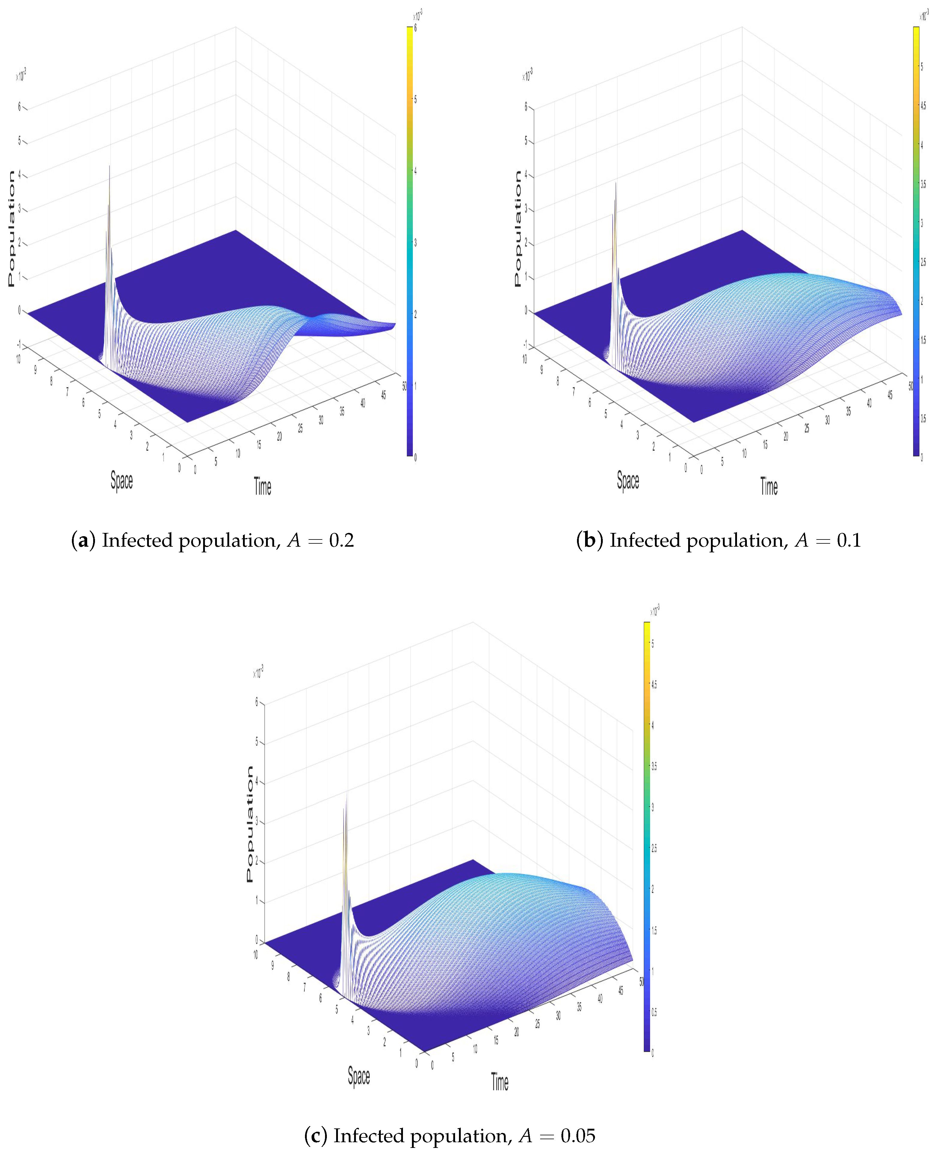
The parameter A represents the gradient-induced advection effect in the infected population, which significantly influences the spatial and temporal dynamics of the epidemic. Its role is to model the directed movement of the infected individuals toward regions of higher infection density, effectively amplifying the local concentration of infection.

For the infected population (I) in Figure 3a,c, increasing A enhances the spatial propagation of infection, leading to a more distributed infection profile over time. As A increases, infected individuals are more likely to move toward high-density infection regions, resulting in broader spatial spread and a more diffuse infection front. This reduces the intensity of local infection peaks, as the infection becomes less concentrated in any given region. Moreover, for large values of A, the infected population exhibits a significant reduction in localized infection waves, favoring a smoother and more gradual infection distribution. This behavior is critical in controlling highly localized outbreaks, as it facilitates the redistribution of infected individuals over the domain, thereby diminishing the likelihood of sharp epidemic spikes.

On the other hand, the effect of A on the recovered population (R) is indirectly governed by its impact on the infected population. As A increases, the spatial redistribution of infection results in a slower but more homogeneous recovery process. Since the infected individuals are less concentrated in specific areas, the recovery dynamics become less abrupt, leading to a more gradual rise in the recovered population. This diffusion of infection also prolongs the epidemic’s duration, as the reduced local infection intensity delays the overall recovery process. However, the broader spread of infection under large values of A ensures that the epidemic does not exhibit high-amplitude peaks, but instead transitions smoothly to the endemic state or complete recovery over a longer time horizon.

Figure 3. Impact of the gradient-induced advection coefficient A on the susceptible (S), infected (I), and recovered (R) populations for higher values of A. Panels (a–c) show the temporal evolution of the infected population at A = 0.2, A = 0.1, and A = 0.05, respectively, demonstrating that higher advection leads to broader spatial distribution of infection and smoother infection waves.

Figure 3. Impact of the gradient-induced advection coefficient A on the susceptible (S), infected (I), and recovered (R) populations for higher values of A. Panels (a–c) show the temporal evolution of the infected population at A = 0.2, A = 0.1, and A = 0.05, respectively, demonstrating that higher advection leads to broader spatial distribution of infection and smoother infection waves.

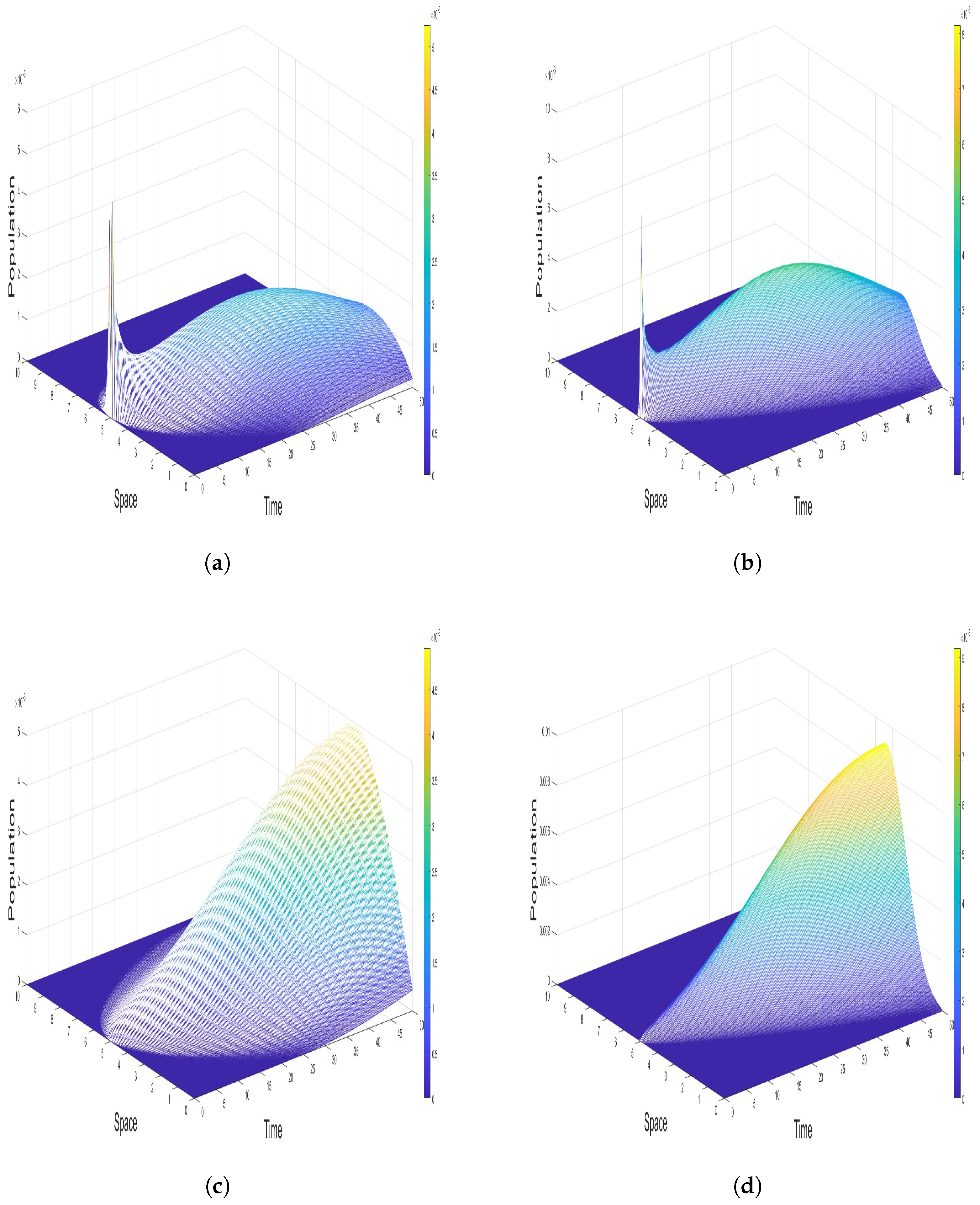
4.3. Impact of $D_S,D_I,D_R$

Figure 4 illustrates the impact of varying diffusion coefficients $D_S$, $D_I$, and $D_R$ on the spatial dynamics of the infected and recovered populations. The diffusion terms $D_S$, $D_I$, and $D_R$ represent the random movement of the susceptible, infected, and recovered individuals, respectively, across the spatial domain, modeled by the Laplacian operator ${\nabla }^2$. This diffusion process plays a pivotal role in spreading the population densities over space, thereby influencing the disease dynamics.

In Figure 4a,b, we observe the infected population for two sets of diffusion coefficients: $D_S=D_I=D_R=0.05$ and $D_S=D_I=D_R=0.01$, respectively. Panel (a) shows that when the diffusion coefficients are higher, the infected population spreads more uniformly across the domain. The infection peak is less concentrated, indicating that higher diffusion rates facilitate faster and more extensive spatial propagation of the disease. This results in a broader spatial infection wave, where the infection diffuses into neighboring regions, reducing local infection peaks. The diffusion process smooths out the infection density, making the epidemic less localized and mitigating sharp spikes in infected individuals. In contrast, Figure 4b demonstrates the effect of lower diffusion coefficients. The infection remains more localized, with less pronounced spatial spread, leading to higher infection concentrations in specific areas. The lower diffusion rate slows down the movement of infected individuals, resulting in steeper infection peaks. This indicates that low diffusion coefficients allow the infection to stay concentrated in certain regions, thereby increasing the intensity of local outbreaks and potentially leading to more severe epidemic waves.

Similarly, Figure 4c,d depict the recovered population under the same diffusion coefficient settings. In panel (c), with higher diffusion coefficients, the recovered population exhibits a more evenly distributed recovery over space. The recovery wave is smoother and covers a wider spatial region, reflecting the broader infection spread due to increased diffusion. The higher diffusion rates ensure that recovered individuals are more uniformly distributed across the domain, which prevents any localized recovery surges and results in a gradual transition to the recovered state. Figure 4d shows the effect of lower diffusion coefficients on the recovered population. With $D_S=D_I=D_R=0.01$, the recovery process is more concentrated, similar to the infected population dynamics in Figure 4b. The lower diffusion rates confine the recovered population to specific regions, where the infection was initially concentrated. As a result, the recovery process is slower and more localized, and it mirrors the more intense and localized infection dynamics seen in Figure 4b. Higher diffusion rates ($D_S=D_I=D_R=0.05$) lead to a more dispersed infection and recovery process, reducing local outbreak intensities and promoting a smoother transition across the spatial domain. In contrast, lower diffusion rates ($D_S=D_I=D_R=0.01$) result in more concentrated and intense infection peaks, with the recovery process similarly confined to localized regions. The balance between diffusion and infection dynamics determines the spatial heterogeneity of the epidemic and the effectiveness of intervention strategies.

5. Long-Term Behavior of the Model

We have simulated the model for exploring the dynamics (particularly the long-term behavior of the system) utilizing selective values of the parameters. To numerically explore the stability of the infection-free equilibrium of the model, we have assumed values of the parameters from Table 2. As a general rule of thumb, the threshold within this case is less than unity. The obtained results are provided in Figure 5, from which conclusions about the stability of the DFE can be easily obtained (values given in

Table 3. Values of the parameters used in simulation to explain the dynamics of the solution around the disease-free equilibrium (Sample 1).

Parameters	Values	Parameters	Values
$\beta$	0.225	B	0.02
$\gamma$	0.41	$D_S$	0.01
$\alpha$	0.05	$D_S$	0.01
A	100	$D_S$	0.01

).

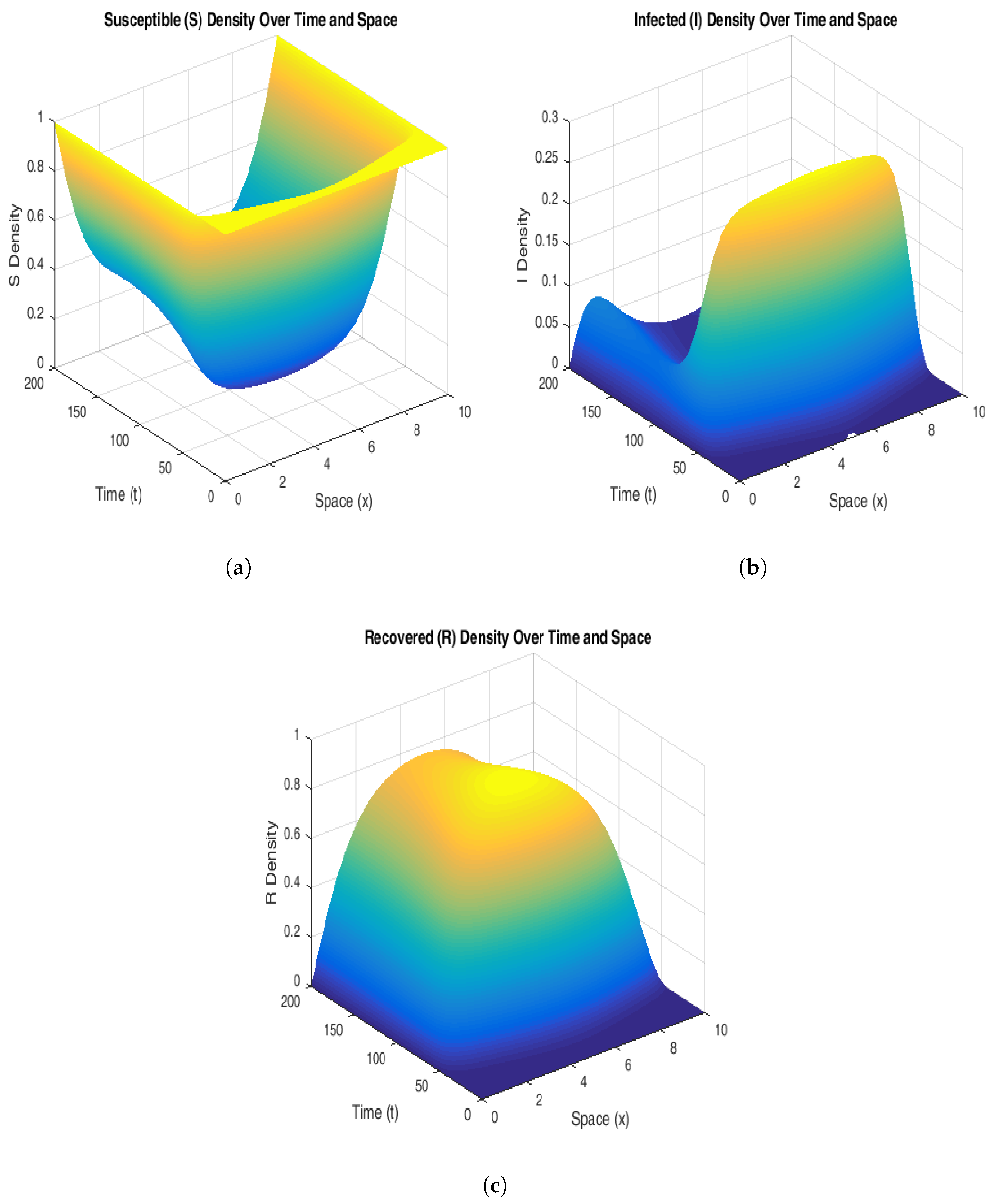
To explain the stability of the endemic equilibrium, we have chosen values of the parameters from Table 3, and this assures that the basic reproduction number is below one. As usual, for $R_0<1$, the endemic equilibrium is stable, and in our case, Figure 6 supports this claim. The susceptible population declines rapidly in the regions of high initial infection, stabilizing at a lower level as the system reaches endemic equilibrium. The infected population shows persistent peaks that propagate spatially, signifying that the disease maintains a consistent presence in the population over time. This persistence highlights the system’s inability to naturally revert to a disease-free state without external intervention. The recovered population increases steadily, following the spatial infection waves, suggesting that immunity builds in previously infected regions.

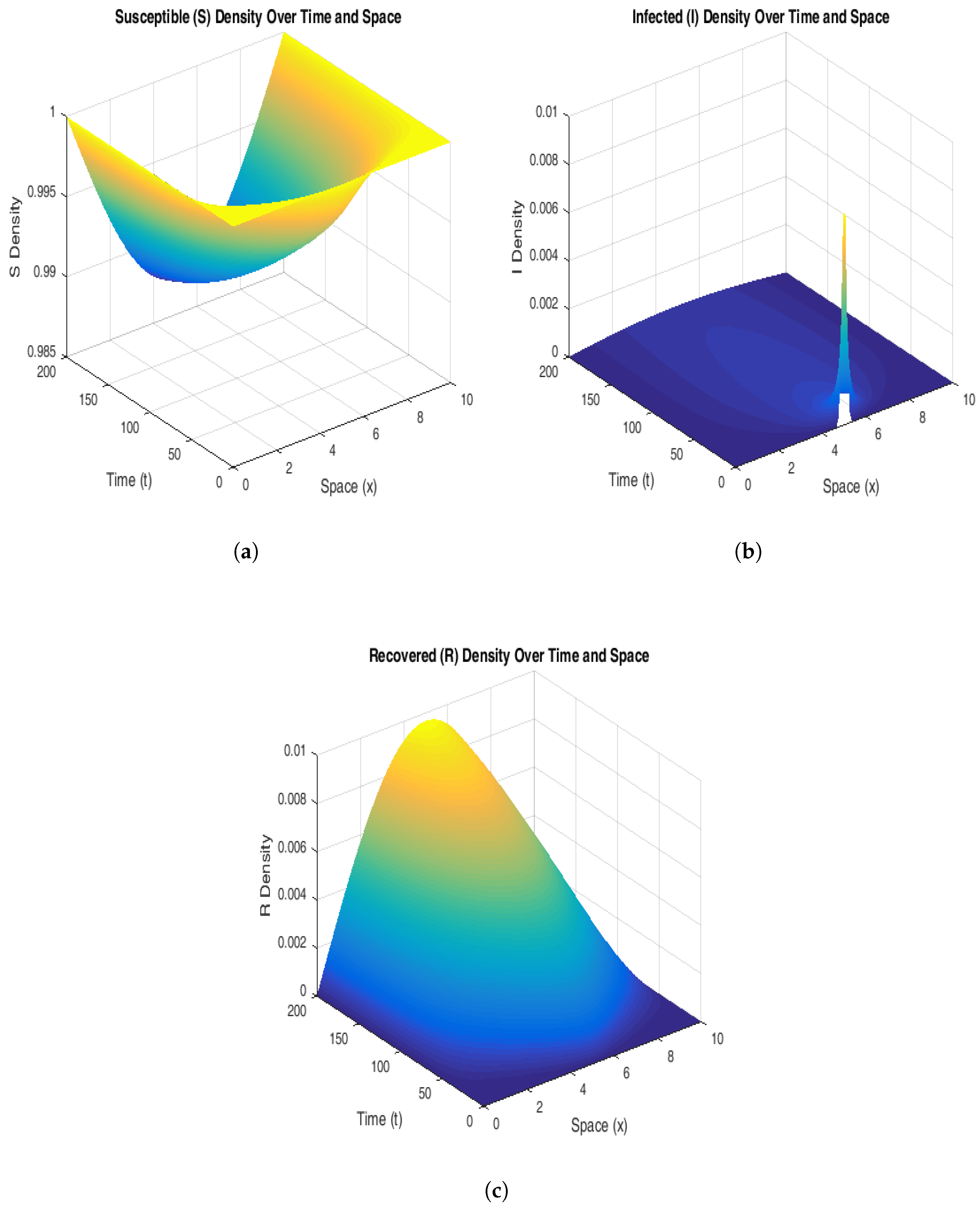
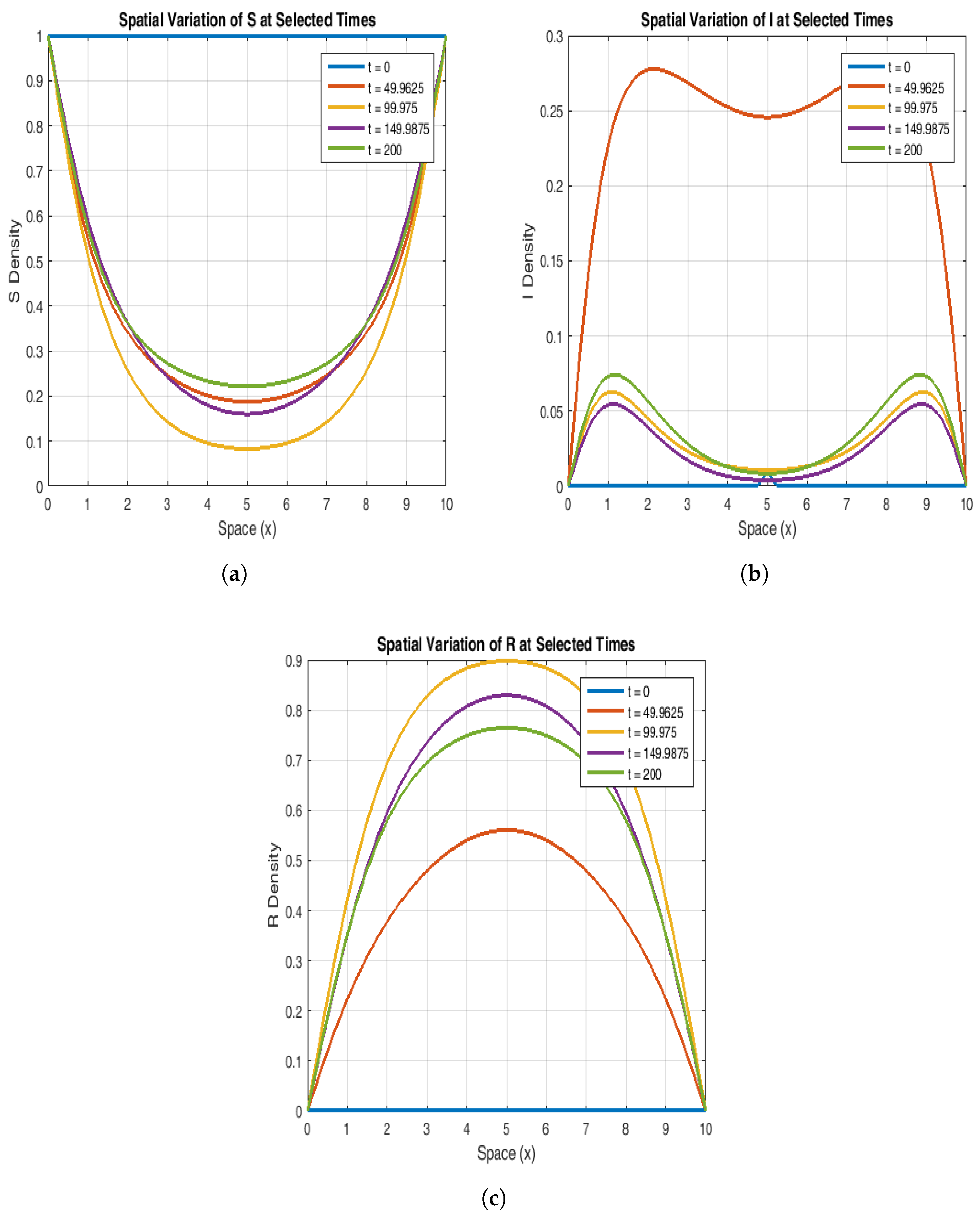
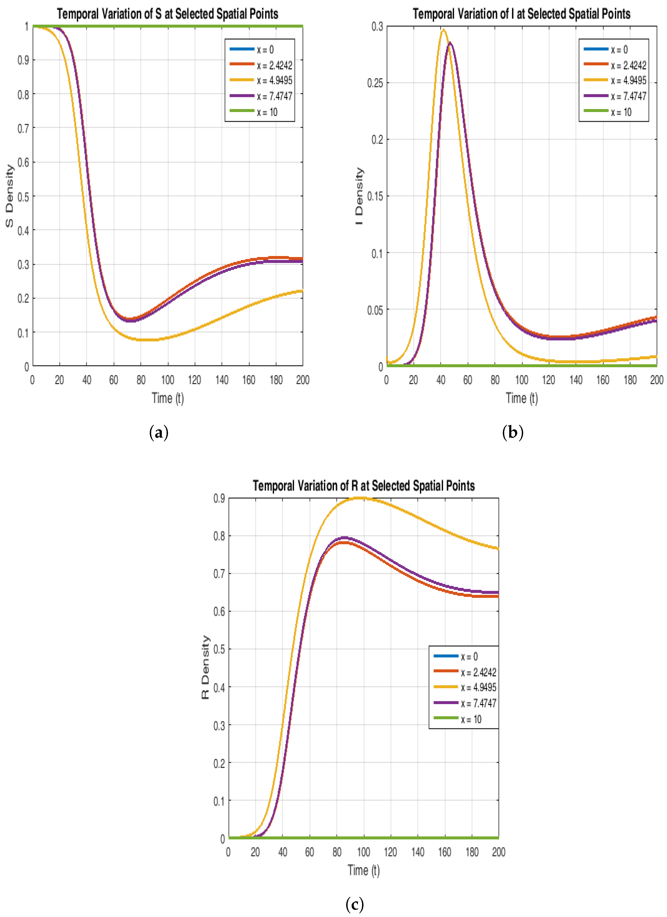
To explain further the stability of the endemic equilibrium, in Figure 7 and Figure 8, we have chosen curves from these 3D plots by fixing the space variable x and time t, respectively. The susceptible population starts at a maximum value (S = 1) uniformly across the spatial domain and decreases over time as the infection grows. As the infection propagates, the susceptible population decreases particularly in the middle of the spatial domain. The susceptible population stabilizes itself over time, flattening out and reaching the equilibrium state. Figure 7b and Figure 8b suggest that at t = 0, the infected population shows a peak at the center of the spatial domain, and as time progresses, the curves become smooth. This shows that the infection spreads with a decreasing intensity. However, when time evolves even more, the population stabilizes itself and reaches the desired endemic equilibrium. Figure 7c and Figure 8c explain that the recovered population increases significantly over time and exhibits a peak at the center of the spatial domain and finally stabilizes itself to the endemic steady state (values given in

Table 4. Values of the parameters used in simulation to explain the dynamics of the solution around the disease-free equilibrium (Sample 2).

Parameters	Values	Parameters	Values
$\beta$	0.3	B	0.02
$\gamma$	0.1	$D_S$	0.01
$\alpha$	0.05	$D_S$	0.01
A	100	$D_S$	0.01

).

The choice of $x=10$ corresponds to the upper boundary of the spatial domain and is used here to illustrate the model’s behavior at the domain edge. This location is particularly relevant due to the influence of the advection term $A·\nabla I$, which drives the infection toward higher spatial indices. As such, the accumulation and amplification of the infected population near $x=10$ can be significant when A is large. In the original parameter set ($B=0.02$, $A=100$), this amplification is further exacerbated by the nonlinear term $-B{I}^3$, which fails to counterbalance the rapid infection growth, especially when the infected population is already large. This leads to numerical overflow and nonphysical results at early time steps. In contrast, the modified parameters ($B=0.01$, $A=0.1$) produce a smoother and more physically realistic evolution, confirming the sensitivity of the system to these coefficients, particularly near domain boundaries.

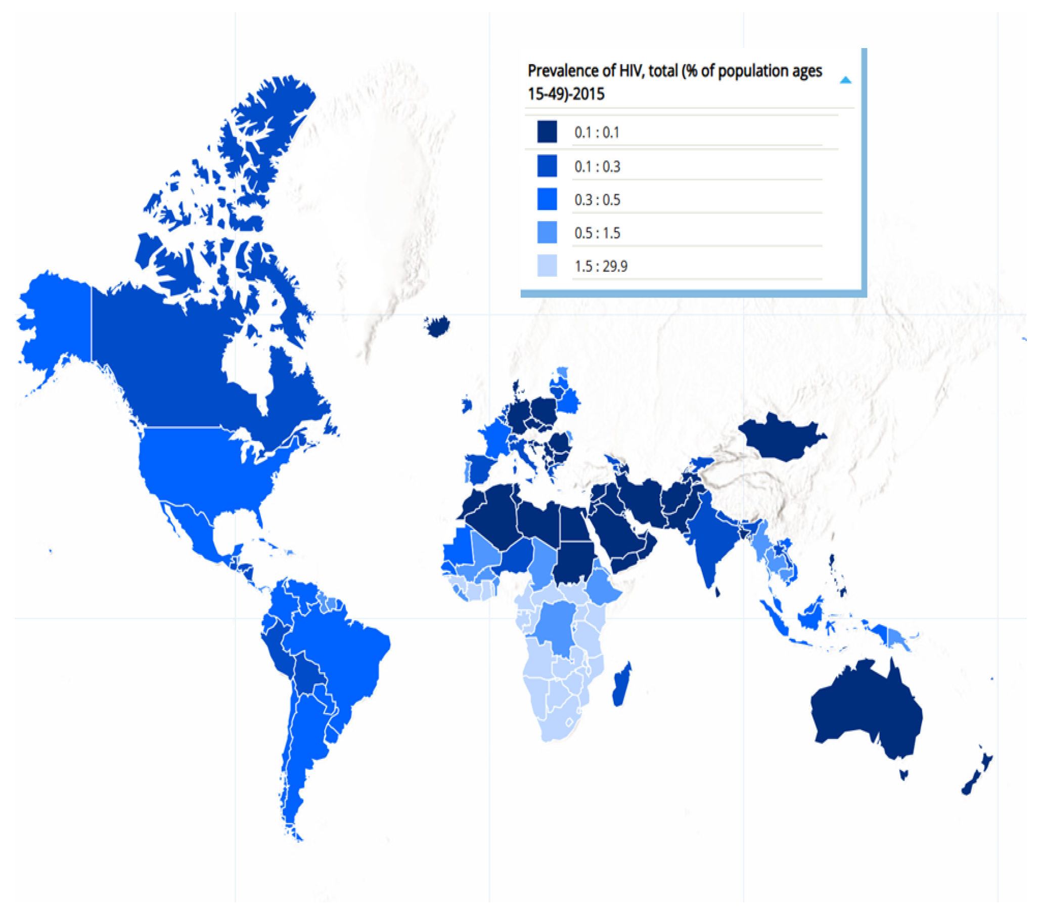
6. Application for AIDS Data

We developed a time-dependent compartmental model to analyze global HIV/AIDS prevalence trends from 1990 to 2022 (Figure 9). The explicit ODE system used in curve fitting is now provided in Section 6. The model is,

$$\begin{array}{cc}\hfill {\displaystyle \frac{dS}{dt}}& =-\beta \left(t\right)SI-\mu S,\hfill \\ \hfill {\displaystyle \frac{dI}{dt}}& =\beta \left(t\right)SI-(\gamma +\alpha \left(t\right))I-B\left(t\right)I^3+AI,\hfill \\ \hfill {\displaystyle \frac{dR}{dt}}& =\gamma I-\nu R.\hfill \end{array}$$

This simplified model omits spatial diffusion and gradient terms due to the global, nonspatial nature of the UNAIDS data.

The soliton-based SIR framework employed in this study includes nonlinear saturation effects (e.g., the $-B{I}^3$ term) and growth modulation ($+AI$), which are suitable for capturing broad epidemic dynamics.

Figure 9. Global HIV/AIDS dynamics.

Figure 9. Global HIV/AIDS dynamics.

The model was calibrated against normalized prevalence data from UNAIDS [27] using World Bank population estimates [28] for conversion to infection fractions. Parameter optimization prioritized recent data through temporal weighting, with validation via out-of-sample testing (Figure 10).

Figure 10. Global HIV/AIDS dynamics: model vs. historical Data.

Figure 10. Global HIV/AIDS dynamics: model vs. historical Data.

7. Conclusions

This study introduces a significant extension to the classical SIR model by embedding soliton-like dynamics and gradient-induced diffusion, providing a robust framework for understanding the spatiotemporal spread of infectious diseases in structured populations. By integrating advection–diffusion mechanisms, the model captures the intricate spatial gradients of infection, enabling the transition from localized epidemic peaks to broadly distributed infection fronts. The soliton-embedded dynamics enhance the stability of infection waves, accurately representing persistent infection hotspots and reflecting the spatiotemporal characteristics observed in real-world disease outbreaks.

The results emphasize the critical role of spatial diffusion and advection in shaping epidemic dynamics. Gradient-induced diffusion disperses infection waves across the spatial domain, reducing the intensity of localized outbreaks and redistributing the epidemic burden. Higher diffusion coefficients lead to smoother, more uniform infection and recovery profiles, while lower coefficients intensify outbreaks, confining them to specific regions. These findings underscore the delicate balance between diffusion and infection dynamics in mitigating localized epidemic peaks and managing spatial heterogeneity.

Parameter sensitivity analysis reveals the significant influence of epidemiological factors such as the transmission rate ($\beta$), recovery rate ($\gamma$), and damping term ($\alpha$). Lower transmission rates delay the epidemic peak, while higher recovery rates expedite transitions to the recovered state. The damping term moderates the persistence of infections, illustrating how the model dynamically responds to changes in key parameters. Stability analysis further highlights the conditions for disease-free and endemic equilibria, with the reproduction number $R_0$ playing a pivotal role. For $R_0<1$, the disease-free equilibrium remains globally stable, while $R_0>1$ drives the system toward endemic stability, ensuring consistency with theoretical predictions.

The model’s applicability is demonstrated through its application to AIDS dynamics among the world population over the last 25 years. Calibrated to the prevalence rate, the model successfully captures the temporal progression of infection, aligning with observed epidemiological patterns. This computational framework provides a valuable tool for exploring adaptive strategies, such as targeted interventions and vaccination campaigns, for managing infectious diseases in spatially heterogeneous and mobile populations.

8. Remarks and Future Recommendations

•

The inclusion of a cubic nonlinear term $B{I}^3$ captures saturation effects, preventing unbounded infection growth in high-density regions.

•

Neumann boundary conditions ensure population consistency and can be replaced by Dirichlet conditions for populations interacting across spatial borders.

•

The advection–diffusion coupling models wavefronts of infection and recovery, capturing spatial heterogeneity and complex wave-like behavior.

•

The model is well suited for bifurcation analysis, offering insight into regime transitions such as localized versus widespread infection.

References

- Levkov, D.G.; Maslov, V.E.; Nugaev, E.Y. Chaotic solitons in driven sine-Gordon model. Chaos Solitons Fractals 2020, 139, 110079. [Google Scholar] [CrossRef]
- Tozzi, A. Approaching Electroencephalographic Pathological Spikes in Terms of Solitons. Signals 2024, 5, 281–295. [Google Scholar] [CrossRef]
- Lü, Z.; Zhang, H. Soliton like and multi-soliton like solutions for the BoitiLeonPempinelli equation. Chaos Solitons Fractals 2004, 19, 527–531. [Google Scholar] [CrossRef]
- Liu, G.; Qi, H.; Chang, Z.; Meng, X. Asymptotic stability of a stochastic May mutualism system. Comput. Math. Appl. 2020, 79, 735–745. [Google Scholar] [CrossRef]
- Tran, K.Q.; Yin, G. Optimal harvesting strategies for stochastic ecosystems. IET Control Theory Appl. 2017, 11, 2521–2530. [Google Scholar] [CrossRef]
- Ma, T.; Meng, X.; Chang, Z. Dynamics and optimal harvesting control for a stochastic one-predator-two-prey time delay system with jumps. Complexity 2019, 2019, 5342031. [Google Scholar] [CrossRef]
- Zhao, H.; Gong, Z.; Gan, K.; Gan, Y.; Xing, H.; Wang, S. Supervised kernel principal component analysis-polynomial chaos-Kriging for high-dimensional surrogate modelling and optimization. Knowl.-Based Syst. 2024, 305, 112617. [Google Scholar] [CrossRef]
- Yang, R.S.; Li, H.B.; Huang, H.Z. Multisource information fusion considering the weight of focal element’s beliefs: A Gaussian kernel similarity approach. Meas. Sci. Technol. 2023, 35, 025136. [Google Scholar] [CrossRef]
- Han, L.; Xu, S.; Chen, R.; Zheng, Z.; Ding, Y.; Wu, Z.; Li, S.; He, B.; Bao, M. Causal associations between HbA1c and multiple diseases unveiled through a Mendelian randomization phenome-wide association study in East Asian populations. Medicine 2025, 104, e41861. [Google Scholar] [CrossRef]
- Din, A. The stochastic bifurcation analysis and stochastic delayed optimal control for epidemic model with general incidence function. Chaos Interdiscip. J. Nonlinear Sci. 2021, 31, 12. [Google Scholar] [CrossRef] [PubMed]
- Dong, Y.; Lin, T. Dynamics of a stochastic rumor propagation model incorporating media coverage and driven by Lévy noise. Chin. Phys. B 2021, 30, 8. [Google Scholar]
- Din, A.; Li, Y. Lévy noise impact on a stochastic hepatitis B epidemic model under real statistical data and its fractal–fractional Atangana–Baleanu order model. Phys. Scr. 2021, 96, 124008. [Google Scholar] [CrossRef]
- Keeling, M.J.; White, P.J. Targeting vaccination against novel infections: Risk, age and spatial structure for pandemic influenza in Great Britain. J. R. Soc. Interface 2011, 8, 661–670. [Google Scholar] [CrossRef] [PubMed]
- Mohamed, A.; Baaro, G.P.; Gelle, S.J. Assessment of knowledge, attitude and practices (KAPS) of anthrax among Pastoralists in Wajir, Isiolo and Marsabit Counties, Kenya. J. Agric. Sci. Technol. 2019, 9, 56–63. [Google Scholar]
- Habenom, H.; Aychluh, M.; Suthar, D.L.; Al-Mdallal, Q.; Purohit, S.D. Modeling and analysis on the transmission of covid-19 Pandemic in Ethiopia. Alex. Eng. J. 2022, 61, 5323–5342. [Google Scholar] [CrossRef]
- Sun, G.Q.; Li, M.T.; Zhang, J.; Zhang, W.; Pei, X.; Jin, Z. Transmission dynamics of brucellosis: Mathematical modelling and applications in China. Comput. Struct. Biotechnol. J. 2020, 18, 3843–3860. [Google Scholar] [CrossRef]
- Mogaji, H.O.; Adewale, B.; Smith, S.I.; Igumbor, E.U.; Idemili, C.J.; Taylor-Robinson, A.W. Combatting anthrax outbreaks across Nigerias national land borders: Need to optimize surveillance with epidemiological surveys. Infect. Dis. Poverty 2024, 13, 10. [Google Scholar] [CrossRef]
- Gaff, H.D.; Hartley, D.M.; Leahy, N.P. An epidemiological model of Rift Valley fever. Electron. J. Differ. Equ. (Ejde) 2007, 2007, 1–12. [Google Scholar]
- Abellan, J.J.; Richardson, S.; Best, N. Use of spacetime models to investigate the stability of patterns of disease. Environ. Health Perspect. 2008, 116, 1111–1119. [Google Scholar] [CrossRef]
- LeMenach, A.; Legr, J.; Grais, R.; Viboud, C.; Valleron, A.J.; Flahault, A. Modeling spatial and temporal transmission of foot-and-mouth disease in France: Identification of high-risk areas. Vet. Res. 2005, 36, 699–712. [Google Scholar] [CrossRef] [PubMed]
- Din, A.; Li, Y. Ergodic stationary distribution of age-structured HBV epidemic model with standard incidence rate. Nonlinear Dyn. 2024, 112, 9657–9671. [Google Scholar] [CrossRef]
- Din, A.; Li, Y. Controlling heroin addiction via age-structured modeling. Adv. Differ. Equ. 2020, 2020, 521. [Google Scholar] [CrossRef]
- Murray, J.D. Mathematical Biology I: An Introduction; Springer: Berlin/Heidelberg, Germany, 2002. [Google Scholar]
- Britton, N.F. Reaction-Diffusion Equations and Their Applications to Biology; Academic Press: Cambridge, MA, USA, 1986. [Google Scholar]
- Han, C.; Wang, Y.L.; Li, Z.Y. A high-precision numerical approach to solving space fractional Gray-Scott model. Appl. Math. Lett. 2022, 125, 107759. [Google Scholar] [CrossRef]
- Che, H.; Wang, Y.L.; Li, Z.Y. Novel patterns in a class of fractional reaction-diffusion models with the Riesz fractional derivative. Math. Comput. Simul. 2022, 202, 149–163. [Google Scholar] [CrossRef]
- UNAIDS. Global AIDS Monitoring 2023; Joint United Nations Programme on HIV/AIDS: Geneva, Switzerland, 2023. [Google Scholar]
- World Bank. World Population Prospects; World Bank Group: Washington, DC, USA, 2023. [Google Scholar]
Figure 1.
Influence of infection rate, recovery rate, and damping rate on the temporal dynamics of susceptible, infected, and recovered populations, illustrating how parameter changes affect epidemic progression: (a) Susceptible population, . (b) Recovered population, . (c) Infected population, .
Figure 2.
Impact of the gradient-induced advection coefficient A on the susceptible (S), infected (I), and recovered (R) populations for lower values of A. Panels (a–c) show the temporal evolution of the recovered population at A = 0.2, A = 0.1, and A = 0.05, respectively, illustrating how lower advection slows infection spread and recovery dynamics.
Figure 4.
Effect of diffusion coefficients on the spatial distribution of infected and recovered populations, comparing scenarios of high versus low diffusion and their impact on infection spread and recovery patterns: (a) Infected population, . (b) Infected population, . (c) Recovered population, . (d) Recovered population, .
Figure 5.
The plot shows the dynamics of the susceptible (a), infected (b), and recovered (c) compartments around the disease-free equilibrium for selected values of the parameters.
Figure 6.
The plot shows the dynamics of the susceptible (a), infected (b), and recovered (c) compartments around the endemic equilibrium for selected values of the parameters, ensuring .
Figure 7.
The plot shows the dynamics of susceptible (a), infected (b), and recovered (c) compartments at the selected values of time t.
Figure 8.
The plot shows the dynamics of susceptible (a), infected (b), and recovered (c) populations at the selected values of space variable x.