Article

A Discrete Grey Seasonal Model with Fractional Order Accumulation and Its Application in Forecasting the Groundwater Depth

1
School of Management Science and Engineering, Shandong University of Finance and Economics, Jinan 250014, China
2
Institute of Marine Economics and Management, Shandong University of Finance and Economics, Jinan 250014, China
3
College of Management Engineering and Business, Hebei University of Engineering, Handan 056038, China
*
Author to whom correspondence should be addressed.
Fractal Fract. 2025, 9(2), 117; https://doi.org/10.3390/fractalfract9020117
Submission received: 8 December 2024 / Revised: 18 January 2025 / Accepted: 12 February 2025 / Published: 13 February 2025

Abstract

Influenced by the hydrogeological structure and other factors, the change in groundwater depth shows seasonal fluctuation characteristics. Human activities have disrupted the long-term stable pattern of groundwater change, which makes the short-term prediction of groundwater depth important. To cope with the emergence of short-term groundwater prediction scenarios, for the first time, a discrete grey seasonal model with fractional order accumulation is proposed in this paper (FDGSM(1,1)). First, the DGM(1,1) model, which has a relative advantage over fluctuating data, was chosen as the basis for the transformation of the proposed model. Then, the fractional order accumulation operator is used to reduce the seasonal fluctuations in the data series. Finally, grey seasonal variables are introduced to construct the time response function. The proposed model has the basic properties of the traditional grey forecasting model, which is proven to be stable and seasonal. Additionally, the prediction performance of the proposed model is verified in a real scenario of Handan groundwater. This paper expands the seasonal prediction field of the grey prediction model, enriches the research system of the grey system theory and fractional order, and has a positive influence on the short-term prediction of groundwater depth.

1. Introduction

Groundwater underpins the development of society. More than two billion people worldwide rely on groundwater as their primary water resource, and more than half of the irrigation water for food crops comes from groundwater [1]. Groundwater is also an important part of the earth’s water circulation system. However, the rising demand for water has led to the overexploitation of groundwater [2,3]. Combined with pollution from human activities, less groundwater resources are directly available than expected [4]. In the case of limited groundwater resources, the main approach is strengthening the management of groundwater resources [5,6]. It is well known that agricultural irrigation consumes a huge amount of water, especially, in arid areas, where a large proportion of irrigation water comes from groundwater [7,8]. Optimization of planting and development of water-saving irrigation has become a recognized way of alleviating groundwater pressure [9,10]. Therefore, accurate assessment and prediction of groundwater is an important part of groundwater management. Many scholars have made great efforts to observe groundwater; for example, satellites have been used to assess changes in groundwater [11]. The vulnerability of groundwater to contamination has been assessed and mapped [12]. Based on drivers-pressures-states-impact-response assessment framework, the groundwater sustainability index in China was assessed [13]. Remote sensing technology was used to estimate the impact of crops on groundwater [14].
The above methods are effective for the study of groundwater in large areas, but they are not accurate in the assessment of regional groundwater. In recent years, the improvement of underground monitoring of well networks has provided convenience for the direct observation of groundwater changes. The study on the depth of groundwater can help to understand the influence of groundwater more comprehensively. The rise or fall of the groundwater has different effects on our living environment [15,16,17]. Therefore, an accurate prediction of groundwater depth is more conducive to maintaining the balance of the environment. Conventional mathematical modelling, intelligent algorithms, and hybrid models are commonly used to predict the groundwater depth. An adaptive neuro-fuzzy inference system and combined to predict groundwater depth and potential [18,19]. Hybrid soft-computing techniques and integrated wavelet-support vector machines were applied to groundwater depth prediction [20,21]. An improved Bayesian model realizes groundwater prediction under uncertain conditions [22]. Although the use of intelligent algorithms has greatly improved the accuracy of predictions, it is still difficult to meet the forecast requirements in the case of insufficient data.
Due to the non-direct observation of groundwater and the late construction of underground monitoring of the well network, complete and continuous groundwater depth time series data are not readily available. The grey system theory provides a solution to the problem of small samples [23,24]. The grey model has been widely applied in energy, biology, environment, computer, and other fields because of its predictive performance in uncertain systems [25,26,27,28]. Grey prediction models are an important part of prediction science along with machine learning, artificial intelligence, and other methods [29,30,31]. The discrete grey model solves the problem of the transformation of the traditional grey model from the whitening form to the discrete form [32]. In order to satisfy the new information priority principle of the grey system theory, a fractional order accumulation grey model was proposed [33]. The above-mentioned grey models have good performance in dealing with time series with little fluctuation but for a time series with great fluctuation, the prediction accuracy is not satisfactory. Therefore, a grey season model is proposed to study the seasonal fluctuation sequence. The early form of the grey seasonal model was a hybrid model, which was combined with a traditional seasonal model such as ARIMA [34]. Later, the grey seasonal model was widely studied, resulting in the proposed seasonal discrete grey model for fashion retailing [35]. The seasonal GM(1,1) model was applied to the forecasting of power generation [36]. The seasonal FGM(1,1) model was employed to solve air quality problems [37]. The novel discrete grey model improves the ability of the grey discrete model to deal with fluctuation data [38]. But these grey season models do not capture the seasonal characteristics very well. The groundwater time series has the characteristics of seasonal fluctuation and is a typical small sample because it is not easy to observe. Therefore, a discrete grey season model with fractional order accumulation (FDGSM(1,1)) was proposed to analyze the groundwater in Handan. Compared to previous grey prediction models, the main innovations of the proposed model in this paper are as follows:
(1)
Seasonal attributes of the grey prediction model are improved. Traditional grey forecasting models are weak in handling seasonal fluctuation data due to sample size limitations. To ameliorate this problem, seasonal variables are introduced into the proposed model. A fractional order accumulation operator is used to reduce the effect of seasonal data fluctuations.
(2)
Properties of the proposed model are proved. The proposed model is shown to be a derivative of the traditional grey prediction model, indicating that the new model has the fundamental properties and advantages of the grey prediction model. In addition, the seasonality and stability of the proposed model are demonstrated.
(3)
The performance of the proposed model is validated in a real case of Handan groundwater. The prediction performance of the proposed model is verified by the actual groundwater scenario in Handan. The introduction of real groundwater scenarios tests the practical application value of the proposed model.
The remainder of the paper is organized as follows: Section 2 presents an actual groundwater scenario. Section 3 describes the establishment process of the proposed model. Section 4 applies the proposed model to the Handan groundwater scenario. Section 5 discusses and summarizes the paper.

2. Study Area and Data Description

This section presents a real groundwater application scenario. The scenario includes the geographic location, administrative area, and quantitative analysis of groundwater.

2.1. Study Area

Handan is located in the southernmost part of the Hebei province, with a total area of 12,073.8 km2. Handan’s administrative district includes 6 urban districts, 11 counties, and 1 county-level city (Figure 1). Handan topography from the west to the east has a step-like decline, complex and diverse geomorphologic types. The western region belongs to the Taihang Mountains, mainly including She County, Wuan (county-level city), and Fengfeng (part of the urban area). The rest of the eastern part belongs to the North China Plain. Handan has a warm temperate continental monsoon climate with an average annual temperature of 13.5 °C.
The North China Plain where Handan is located suffers from serious groundwater deficiency. According to the statistics, the North China Plain draws about 5.5 billion m3 of groundwater annually. At present, the accumulated groundwater deficit in North China Plain is about 180 billion m3, making it the world’s largest underground water drop funnel area. Handan is a central city in North China, bordering Shaxi, Shangdong, and Henan provinces in addition to Hebei province. Therefore, the study of groundwater in the Handan area has important guiding significance for the whole North China Plain.

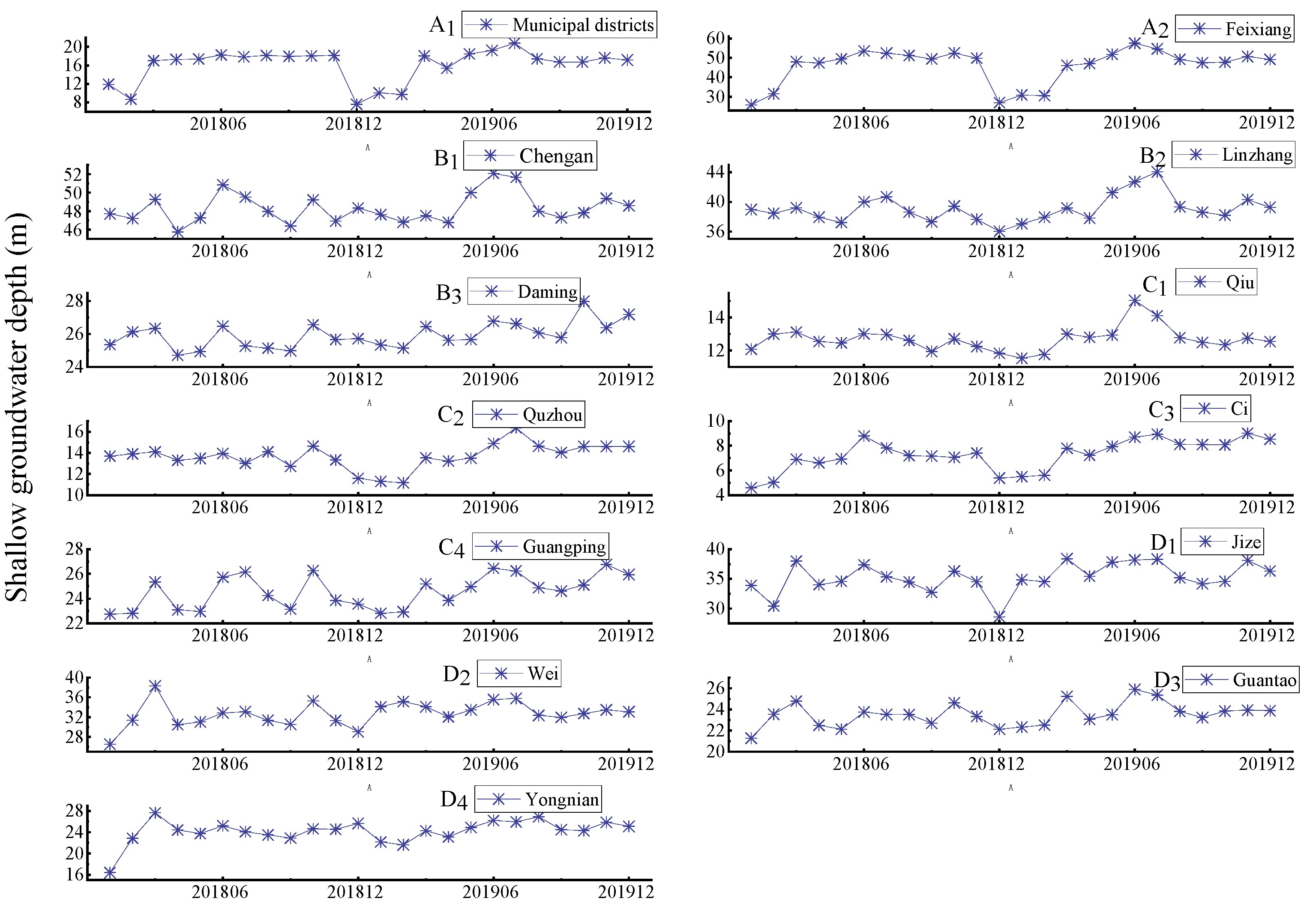
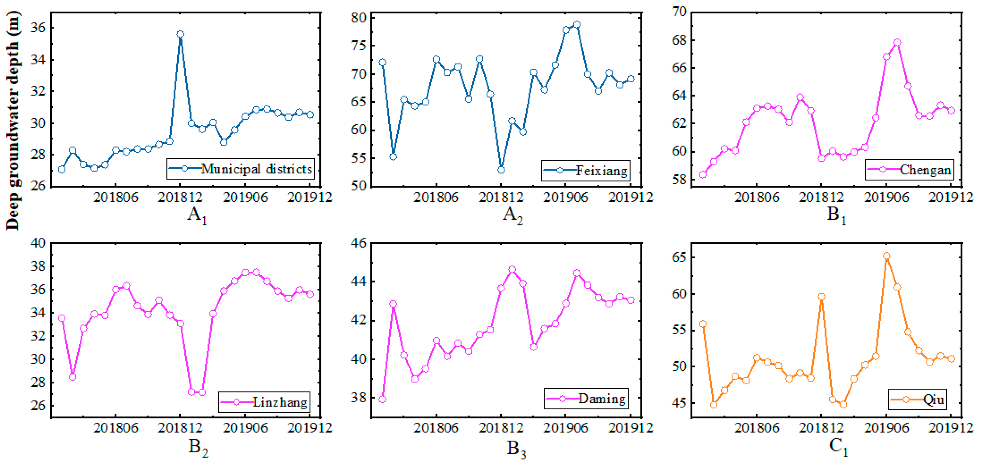
2.2. Data Description
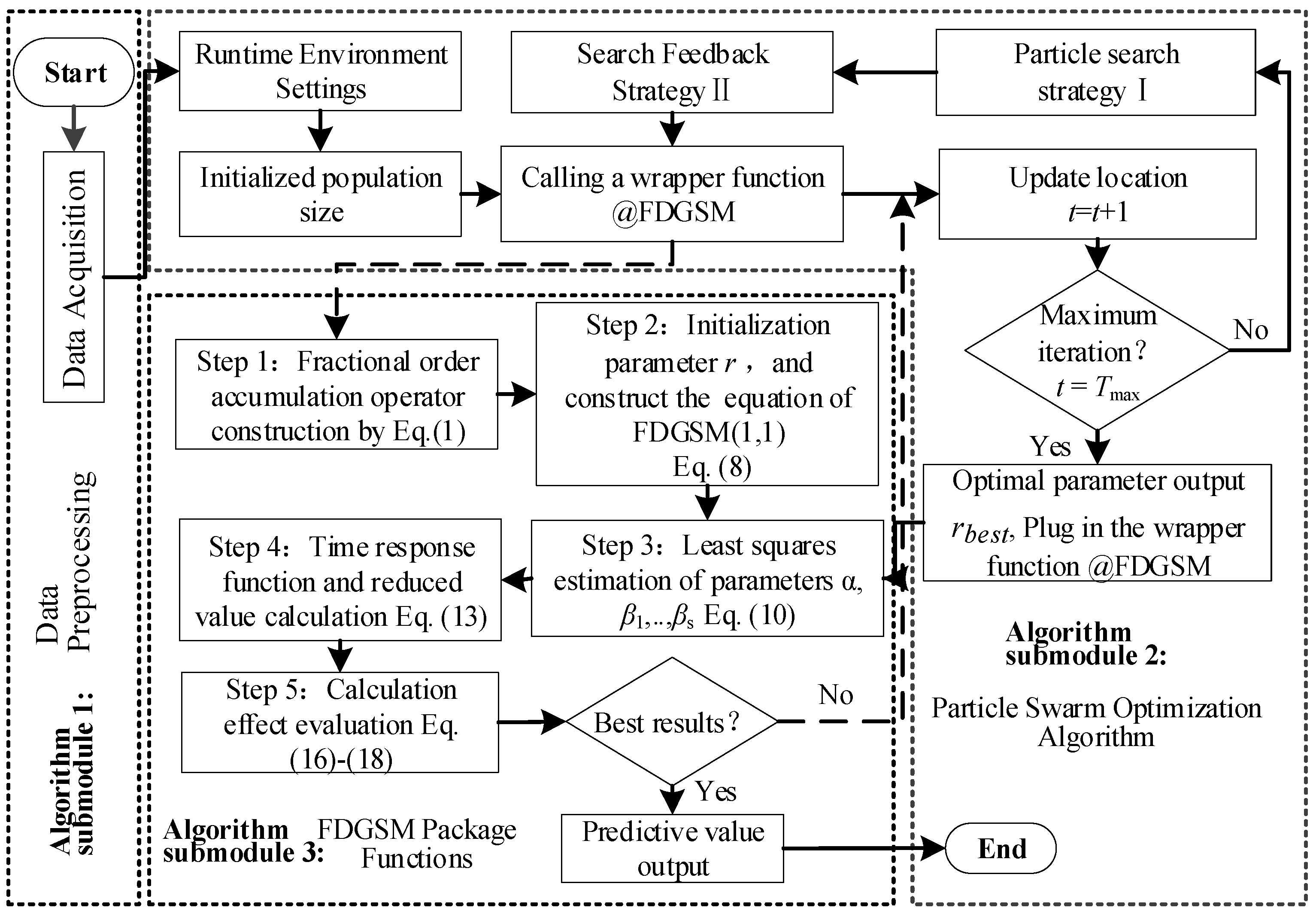
The data on groundwater in the paper are from public government briefs [39]. As the problem of groundwater is a wide societal concern, the government has begun to invest in improving the groundwater monitoring network in recent years. Hence, the data on groundwater depth from 2018 to 2019 are more comprehensive, so groundwater depth data during this period were used for research. The groundwater data of each area in Handan is an average value of the area. In order to comprehensively understand Handan groundwater, shallow and deep groundwater were studied separately. The shallow groundwater data involved 13 counties and districts of Handan, and deep groundwater involved 12. The deep groundwater data of Ci County is not available due to equipment failure. The Municipal districts of Handan include the Fuxing, Congtai, and Hanshan District. Because the groundwater data in these three areas are almost the same, the average of the three regions represents the groundwater data for the Municipal districts. The She County (E1), Wuan (E2), and Fengfeng mining areas (E3) only have data related to the deep groundwater depth from September 2010, which has no research significance. Individual missing data were supplemented by the mean value of data before and after use.
The results of the descriptive statistics of the Handan groundwater depth data are shown in Table 1 and are displayed as average values of groundwater in the Handan area.

3. Method

This section describes the establishment process of the proposed model, provides a heuristic algorithm-based solution for the model parameters, and analyzes the seasonality and stability of the proposed model.

3.1. Discrete Grey Model with Fractional Order Accumulation

Discrete grey models have a comparative advantage in dealing with volatile data. The discrete grey model based on fractional order accumulation is beneficial to extend data processing advantages (FDGM(1,1)). The modelling process for the FDGM(1,1) model is as follows:
Step 1: Fractional order accumulation operator.
Suppose the X ( 0 ) = ( x ( 0 ) ( 1 ) , x ( 0 ) ( 2 ) , , x ( 0 ) ( n ) ) is the original non-negative sequence. The sequence X ( r ) = ( x ( r ) ( 1 ) , x ( r ) ( 2 ) , , x ( r ) ( n ) ) is the r-order fractional accumulation sequence of X ( 0 ) .
The calculation formula of fractional order accumulation is
x ( r ) ( k ) = i = 1 k C k i + r 1 k i x ( 0 ) ( i )
where C r 1 0 = 1 ,   C k k + 1 = 0 ,   C k i + r 1 k i = ( k i + r 1 ) ( k i + r 2 ) ( r + 1 ) r ( k i ) ! .
Step 2: Establishment of grey discrete model.
x ( r ) ( k + 1 ) = α x ( r ) ( k ) + β ( k = 1 , 2 , , n 1 ) ,
is the basic form of fractional order discrete grey model. α is the development coefficient of the discrete grey model, and β is the grey constant.
Step 3: Parameter solving process.
The mathematical recursion is obtained by substituting the sequence data into Equation (2).
x ( r ) ( 2 ) = α x ( r ) ( 1 ) + β x ( r ) ( 3 ) = α x ( r ) ( 2 ) + β x ( r ) ( n ) = α x ( r ) ( n 1 ) + β ,
the matrix form of Equation (3) is Y = C D , where
C = x ( r ) ( 1 ) 1 x ( r ) ( 2 ) 1 x ( r ) ( n 1 ) 1 , Y = x ( r ) ( 2 ) x ( r ) ( 3 ) x ( r ) ( n ) , D = α β ,
the least square method is used to solve the matrix formula, the parameters can be calculated as
α ^ β ^ = ( C T C ) 1 C T Y .
Step 4: Derivation of the time response formula.
According to the above steps, the time response of the discrete grey model with fractional order accumulation is deduced. Parameters are substituted into Equation (2), and x 1 ( r ) ( 1 ) = x 1 ( 0 ) ( 1 ) is used as the initial value. The form of the time response is as follow:
x ^ 1 ( r ) ( k + 1 ) = α ^ k x ( 0 ) ( 1 ) + 1 α ^ k 1 α ^ β ^ ,   k = 1 , 2 , .
The values of k can be substituted into Equation (6), and the fitting and predicted values of the accumulative sequence will be calculated. The newly generated fitting sequence is X ^ ( r ) = { x ^ ( r ) ( 1 ) , x ^ ( r ) ( 2 ) , , x ^ ( r ) ( n ) } .
Step 5: The cumulative sequence fitting values are restored.
To restore r-order cumulative sequence, r-order subtractive generating operator is used. a ( r ) is the r-subtractive generator of X ^ ( 0 ) . Therefore, for X ^ ( r ) = { x ^ ( r ) ( 1 ) , x ^ ( r ) ( 2 ) , , x ^ ( r ) ( n ) } , the reduction formula is as follows:
a ( r ) X ^ ( r ) = a ( 1 ) X ^ ( r ) ( 1 r ) = { a ( 1 ) x ^ ( r ) ( 1 r ) ( 1 ) , a ( 1 ) x ^ ( r ) ( 1 r ) ( 2 ) , , a ( 1 ) x ^ ( r ) ( 1 r ) ( n ) } ,
where a ( 1 ) x ^ ( r ) ( 1 r ) ( k ) = x ^ ( r ) ( 1 r ) ( k ) x ^ ( r ) ( 1 r ) ( k 1 ) . In Equation (7), the X ^ ( r ) sequence is accumulated by the ( 1 r ) order again, and then reduced by the first-order inversed accumulating generation operator(1-IAGO) [40].
Through the above five steps, the discrete grey model with fractional order accumulation (FDGM(1,1)) is established. Previous studies have shown that the FDGM(1,1) model performs better than the traditional DGM(1,1) model in terms of fitting and prediction accuracy [41]. However, the fitting and prediction accuracy of the two models are reduced when the seasonal fluctuation data are processed.

3.2. The Establishment Process of the FDGSM(1,1) Model

To improve the performance of the FDGM(1,1) model in fitting and prediction accuracy, the FDGSM(1,1) model was proposed. The steps for establishing the new model are as follows:
Step 1: The definition of X ( 0 ) and X ( r ) is the same as in the previous section. The formula for the model is
x ( r ) ( k + 1 ) = α x ( r ) ( k ) + β v ( k + 1 , s ) ,   k = 1 , 2 , .
The new model is abbreviated as FDGSM(1,1), having one variable and fractional order. Where s is the number of cycles in seasonal cycle, and β v ( k + 1 , s ) is the seasonal parameter vector. The angle marker v ( k + 1 , s ) of β is solved according to the following formula:
v ( k + 1 , s ) = s     k mod s = 0 k mod s k mod s 0
For time series data with annual periods, the value of the variable s is 12 indicating the length of the annual period. Correspondingly, for the time series data with quarterly periods, a value of 3 for the variable s indicates the length of the quarterly period.
Step 2: Solve for parameter vector.
Theorem 1.
P = α , β 1 , , β s is set as the parameter vector of the FDGSM(1,1) model. The matrix is listed and solved using the least square method. The solution formula of estimated parameter vector is
P ^ = α ^ , β ^ 1 , , β ^ s = B T B 1 B T Y ,
where
B = x ( r ) ( 1 ) 0 1 0 0 x ( r ) ( 2 ) 0 0 1 0 x ( r ) ( s 1 ) 0 0 0 1 x ( r ) ( s ) 1 0 0 0 x ( r ) ( n 1 ) 1 0 ,   Y = x ( r ) ( 2 ) x ( r ) ( 3 ) x ( r ) ( n ) .
Proof. 
x ( r ) ( k ) is substituted into Equation (8). The following formula is obtained:
x ( r ) ( 2 ) = α ^ x ( r ) ( 1 ) + 0 β ^ 1 + 1 β ^ 2 + 0 β ^ 3 + + 0 β ^ s x ( r ) ( 3 ) = α ^ x ( r ) ( 2 ) + 0 β ^ 1 + 0 β ^ 2 + 1 β ^ 3 + + 0 β ^ s x ( r ) ( s ) = α ^ x ( r ) ( s 1 ) + 0 β ^ 1 + 0 β ^ 2 + 0 β ^ 3 + + 1 β ^ s x ( r ) ( s + 1 ) = α ^ x ( r ) ( s ) + 1 β ^ 1 + 0 β ^ 2 + 0 β ^ 3 + + 0 β ^ s x ( r ) ( n ) = α ^ x ( r ) ( n 1 ) + + 1 β ^ M ( n , s ) + + 0 β ^ s .
Equation (12) is converted to a matrix expression, Y = B P . The least square method is used to solve the estimated parameter vector, P ^ = B T B 1 B T Y . By substituting the estimated parameters into the time response formula of the next step, the fitting value and predicted value of the time series can be obtained. □
Step 3: The time response function.
Theorem 2.
Let P ^ = α ^ , β ^ 1 , , β ^ s be the estimated parameter vector of the FDGSM(1,1). The time response of the seasonal time series can be obtained as follows:
x ^ ( r ) ( k ) = α ^ ( k 1 ) x ( 0 ) ( 1 ) + α ^ k 2 β ^ 2 + j = 3 k α ^ k j β ^ v ( j , s ) ,
and its reduction process is consistent with Equation (7). Therefore, the fitting and predicted values of the seasonal times series are obtained. The final calculation result is expressed as X ^ ( 0 ) = x ^ ( 0 ) 1 , x ^ ( 0 ) 2 , , x ^ ( 0 ) n , x ^ ( 0 ) n + 1 , .
Proof. 
The mathematical induction is employed to prove Equation (13).
When k = 2, according to Equation (8), we obtain
x ( r ) ( 2 ) = α ^ x ( r ) ( 1 ) + β ^ 2 = α ^ x ( 0 ) ( 1 ) + β ^ 2 = α ^ 2 1 x ( 0 ) ( 1 ) + α ^ 2 2 β ^ 2 + j = 3 2 α ^ 2 j β ^ M ( j , s )
Supposing Equation (13) is right when k = i, then k = i + 1 is substituted into Equation (13):
x ( r ) ( i + 1 ) = α ^ x ( r ) ( i ) + β ^ M ( i + 1 , s ) = α ^ α ^ i 1 x ( 0 ) ( 1 ) + α ^ i 2 β ^ 2 + j = 3 i α ^ i j β ^ M ( j , s ) + β ^ M ( j , s ) = α ^ i + 1 1 x ( 0 ) ( 1 ) + α ^ i + 1 2 β ^ 2 + j = 3 i α ^ i + 1 j β ^ M ( j , s ) + α ^ i + 1 i 1 β ^ M ( i + 1 , s ) = α ^ i + 1 1 x ( 0 ) ( 1 ) + α ^ i + 1 2 β ^ 2 + j = 3 i + 1 α ^ i + 1 j β ^ M ( j , s )
Obviously, the hypothesis is true. It is proved that the time response after fractional order accumulation is correct. For the convenience of description, the time response expressions in the following paragraphs refer to that after accumulation, the fitting values obtained need to be reduced. □
Step 4: The mean absolute percentage error (MAPE) is used to detect the model’s performance. In addition, two evaluation metrics, mean absolute error (MAE) and root mean square error (RMSE), are added to assess the performance of the proposed model. The process of calculating the three evaluation indicators is as follows:
MAPE = 1 n k = 1 n x ^ ( 0 ) ( k ) - x ( 0 ) ( k ) x ( 0 ) ( k ) × 100 %
MAE = 1 n k = 1 n x ^ ( 0 ) ( k ) - x ( 0 ) ( k )
RMSE = 1 n k = 1 n ( x ^ ( 0 ) ( k ) - x ( 0 ) ( k ) ) 2
In summary, the modelling process of the proposed model is shown in Figure 2. The flowchart shows the particle swarm algorithm to optimize the FDGSM(1,1) model parameters. The solution framework is universal, i.e., the particle swarm algorithm can be replaced with any heuristic algorithm.

3.3. The Properties of the FDGSM(1,1) Model

To better understand the proposed model, the model’s properties are introduced. Property 1 indicates the consistency and difference between the proposed model and the FDGM(1,1) model. In property 2, the proposed model is employed to fit the general cyclic sequence, and the results show that the model accurately fits the original sequence. The reliability and flexibility of the proposed model are verified.
Property 1.
When s = 1 , the FDGSM(1,1) model is equivalent to the FDGM(1,1) model. Namely, the FDGSM(1,1) model is the more general form of the FDGM(1,1) model.
Proof. 
If s = 1 , seasonal features in the time series data are not captured. According to Equation (9), parameter β in the proposed model is a fixed value, similar to parameter α . Namely, the proposed model is derived from the DGM(1,1) model with fractional order accumulation. This indicates that the FDGSM(1,1) model is more general. □
Property 2.
For the original sequence X ( 0 ) = ( x ( 0 ) ( 1 ) , x ( 0 ) ( 2 ) , , x ( 0 ) ( n ) ) , its periodic characteristics can be described as x ( 0 ) ( k ) = x ( 0 ) ( k + s ) = N M ( k , s ) . That is, some data in a sequence remains the same as the data for the next period or more. Under this situation, the new model can still make accurate predictions using these parameters α ^ = 1 , β ^ i = N M ( i , s ) = N i , i = 1 , 2 , , s and x ^ ( 0 ) ( k ) = x ( 0 ) ( k ) .
Proof. 
Considering that x ( 0 ) ( k ) = x ( 0 ) ( k + s ) = N M ( k , s ) , the sequence can be represented in another form: X ( 0 ) = ( N 1 , N 2 , , N s , N 1 , N 2 , , N s , , N M ( k , s ) ) and
x ( r ) ( k ) = k s i = 1 s C s i + r 1 s i N i , x ( r ) ( k + 1 ) = k s i = 1 s C s i + r 1 s i N i + N 1 k mod s = 0 x ( r ) ( k ) = k M ( k , s ) s i s C s i + r 1 s i N i + i = 1 M ( k , s ) C M ( k , s ) i + r 1 M ( k , s ) i N i , k mod s 0 x ( r ) ( k + 1 ) = k + 1 M ( k + 1 , s ) s i s C s i + r 1 s i N i + i = 1 M ( k + 1 , s ) C M ( k + 1 , s ) i + r 1 M ( k + 1 , s ) i N i
When k mod s = 0 , x ( 1 ) ( k + 1 ) = x ( 1 ) ( k ) + N 1 = x ( 1 ) ( k ) + N M ( k + 1 , s ) can be obtained, conversely, if k mod s 0 and M ( k + 1 , s ) = M ( k , s ) + 1 , x ( 1 ) ( k + 1 ) = x ( 1 ) ( k ) + N M ( k + 1 , s ) can be obtained. N M ( k + 1 , s ) is a cyclic sequence with period s, let k = 1 , 2 , , s , the estimated parameters are obtained α ^ = 1 , β ^ i = N M ( i , s ) = N i . Furthermore, x ^ ( 0 ) ( k ) = x ( 0 ) ( k ) can be obtained based on the FDGSM(1,1). Thus, the property indicates that the proposed model can implement the formal transformation flexibly. At the same time, the reliability of the model is verified in another form. □

3.4. Stability Analysis of the Proposed Model

Stability is the prerequisite for a model to be widely applied. In order to evaluate the stability of the proposed model, the matrix perturbation theory is used to solve the perturbation bounds of the model. By comparing with the perturbation bounds of the traditional discrete grey model, the stability of the proposed model is verified. The procedure of solving and proving the disturbance boundary is as follows:
Theorem 3.
Assuming that A C m × n , b C m , A is the generalized inverse of A. when the column vectors of A are linearly independent, the linear least squares problem A x b 2 = min has a unique solution [42].
Theorem 4.
Assuming that A C m × n , b C m , B = A + E , c = b + k C n . Let the solutions to the linear least squares problem B x c 2 = min and A x b 2 = min be x + h and x , respectively. If r a n k ( A ) = r a n k ( B ) = n and A 2 E 2 < 1 , we have
h k γ E 2 A x + k A + k γ E 2 A r x A
where k = A 2 A , γ = 1 A 2 E 2 , r x = b A x (Wu et al., 2014 [41]).
Theorem 5.
According to the least square formula
B x Y 2 = min
the solution to the FDGSM(1,1) model x ( r ) ( k + 1 ) = α x ( r ) ( k ) + β v ( k + 1 , s ) is x. If only perturbations occur x ^ ( 0 ) ( 1 ) = x ( 0 ) ( 1 ) + ε , then
B ^ = B + Δ B = x ( r ) ( 1 ) 0 1 0 0 x ( r ) ( 2 ) 0 0 1 0 x ( r ) ( s 1 ) 0 0 0 1 x ( r ) ( s ) 1 0 0 0 x ( r ) ( n 1 ) 1 0 + ε 0 0 0 0 r ε 0 0 0 0 C s 3 + r s 2 ε 0 0 0 0 C s 2 + r s 1 ε 0 0 0 0 C n 3 + r n 2 ε 0 0 , Y ^ = Y + Δ Y = x ( r ) ( 2 ) x ( r ) ( 3 ) x ( r ) ( n ) + r ε C 1 + r 2 ε C n 2 + r n 1 ε .
A solution to the least squares problem B ^ x Y ^ 2 = min is x ^ , the perturbation of the solution is Δ x . Hypothesis r a n k ( B ) = r a n k ( B ^ ) = 2 , and B 2 Δ B 2 < 1 , then
Δ x ε k γ k = 1 n 1 C k + r 2 k 1 2 x B + k = 2 n C k + r 2 k 1 2 B + k γ k = 1 n 1 C k + r 2 k 1 2 B γ x B .
Proof. 
Obviously, the column vector of B is linearly independent. Therefore, Equation (21) has a unique solution X = Y B . Due to
Δ Y 2 = ( r ) 2 + C r + 1 2 2 + + C n 2 + r n 1 2 ε 2 = k = 2 n C k 2 + r k 1 2 ε , Δ B T Δ B = [ 1 + ( r ) 2 + C r + 1 2 2 + + C n 2 + r n 1 2 ] ε 2 0 0 0 0 0 0 0 0 0 0 0 0 0 0 0 0 0 0 0 0 0 0 ,
and the maximum eigenvalue of Δ B T Δ B is [ 1 + ( r ) 2 + C r + 1 2 2 + + C n 2 + r n 1 2 ] ε 2 . Therefore Δ B 2 = k = 1 n 1 ( C k + r 2 k 1 ) 2 ε . According to Theorem 4, we have Δ x k γ Δ B 2 B x + Δ Y B + k γ Δ B 2 B γ x B = ε k γ k = 1 n 1 C k + r 2 k 1 2 x B + k = 2 n C k + r 2 k 1 2 B + k γ k = 1 n 1 C k + r 2 k 1 2 B γ x B . Thus, when the disturbance is x ^ ( 0 ) ( 1 ) = x ( 0 ) ( 1 ) + ε , the perturbation bound of the solution is marked as L x ( 0 ) ( 1 ) ,
L x ( 0 ) ( 1 ) = ε k γ k = 1 n 1 C k + r 2 k 1 2 x B + k = 2 n C k + r 2 k 1 2 B + k γ k = 1 n 1 C k + r 2 k 1 2 B γ x B .
Theorem 6.
In the same condition as in the Theorem 5, if only perturbations occur x ^ ( 0 ) ( d ) = x ( 0 ) ( d ) + ε ( d = 2 , 3 , , n 1 ) , the perturbation boundary of the model solution is
L x ( 0 ) ( d ) = ε k γ k = 1 n d C k + r 2 k 1 2 x B + k = 1 n d + 1 C k + r 2 k 1 2 B + k γ k = 1 n d C k + r 2 k 1 2 B γ x B .
If only perturbations occur x ^ ( 0 ) ( n ) = x ( 0 ) ( n ) + ε , the perturbation boundary of the solution is
L x ( 0 ) ( n ) = κ γ ε B .
Proof. 
If only perturbations occur x ^ ( 0 ) ( 2 ) = x ( 0 ) ( 2 ) + ε ,
Δ B = 0 0 0 0 0 ε 0 0 0 0 C s 4 + r s 3 ε 0 0 0 0 C s 3 + r s 2 ε 0 0 0 0 C n 4 + r n 3 ε 0 0 Δ Y = ε r ε C n 3 + r n 2 ε ,
the perturbation boundary of the solution is L x ( 0 ) ( 2 ) = ε k γ k = 1 n 2 C k + r 2 k 1 2 x B + k = 1 n 1 C k + r 2 k 1 2 B + k γ k = 1 n 2 C k + r 2 k 1 2 B γ x B . If only perturbations occur x ^ ( 0 ) ( d ) = x ( 0 ) ( d ) + ε ( d = 3 , 4 , , n 1 ) , the perturbation boundary can be obtained L x ( 0 ) ( d ) = ε k γ k = 1 n d C k + r 2 k 1 2 x B + k = 1 n d + 1 C k + r 2 k 1 2 B + k γ k = 1 n d C k + r 2 k 1 2 B γ x B . If only perturbations occur x ^ ( 0 ) ( n ) = x ( 0 ) ( n ) + ε ,
Δ B = 0 0 0 0 0 0 0 0 0 0 0 0 0 0 0 0 0 0 0 0 0 0 0 Δ Y = 0 0 ε ,
the perturbation boundary of the solution is L x ( 0 ) ( n ) = κ γ ε B . □
According to the above verification process, the perturbation bounds of the solutions of the traditional discrete grey model can be obtained separately.
L x ( 0 ) ( 1 ) = n 1 ε k γ x B + 1 B + k γ 1 B γ x B
L x ( 0 ) ( d ) = ε k γ n d x B + n d + 1 B + k γ n d B γ x B
By comparing Equations (22) and (23) with Equations (25) and (26), respectively, it can be seen that the disturbance bound of the solution of the proposed model is significantly smaller than that of traditional discrete grey model. Thus, the FDGSM(1,1) model solution is more stable.

4. Prediction of Handan Groundwater Depth

In order to analyze the change rule of groundwater depth in Handan, the FDGSM(1,1) model was applied to model and calculate groundwater data. Dataset partitioning is a common practice for testing models and is usually divided into in-sample and out-of-sample [43]. In this paper, the data from January 2018 through December 2019 was divided into two periods: an in-sample dataset (i.e., training) from January 2018 to December 2019, and an out-of-sample dataset (i.e., prediction) from January 2020 to December 2020. When the training error is accepted, the proposed model is considered to have successfully captured the periodic pattern of the dataset. The depth of shallow groundwater and deep groundwater in Handan were analyzed, respectively. The process of fitting and predicting the groundwater depth in Handan is shown in Section 4.1 and Section 4.2.

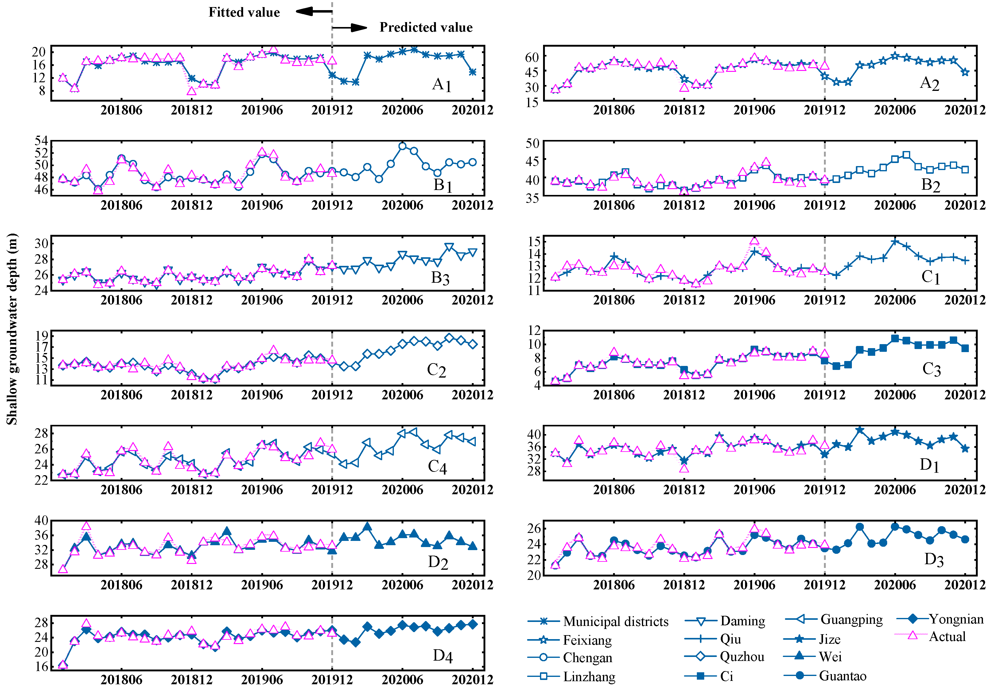
4.1. Prediction of Shallow Groundwater Depth in Handan

This section analyzes the data characteristics of shallow groundwater and discusses the feasibility of the FDGSM(1,1) model. Then, the fitting and prediction of shallow groundwater depth in Handan are completed according to the modelling process of FDGSM(1,1). The specific process is as follows:
Shallow groundwater is easier to monitor than deep groundwater and greatly influenced by social production and life. The depth of shallow groundwater in all counties and districts of Handan is shown in Figure 3. For easy marking and identification, all counties are divided into four groups and are denoted by A, B, C, and D. As shown, the shallow groundwater depth has a seasonal change rule. The shallow groundwater depth is at its lowest level in winter and is affected by the geological conditions in Handan. The depth of groundwater in each county varies greatly. Among them, the shallowest groundwater is Ci County (C3), and the most obvious change is Feixiang district (A2).
Due to the geographical location, the depth of shallow groundwater depth in some areas has similar changes. For example, Municipal districts (A1) is close to Feixiang (A2), and the change rule of shallow groundwater in Municipal is very similar to that in Feixing, as shown in Figure 2. Therefore, intuitive analysis cannot find the difference between the two, it is necessary to carry out quantitative analysis. Particle swarm optimization (PSO) is an optimization algorithm to find the optimal parameter, it is widely used by scholars because of its simple and easy operation. Hence, PSO is employed to solve the optimal order r in the model fitting. According to Equation (10), the estimated parameter values P ^ = α ^ , β ^ v are calculated, and the results of parameter calculation are listed in Table 2. As the experimental data are monthly, the groundwater depth varies completely within the range of the annual cycle. Therefore, the seasonal item is set as s = 12 .
To evaluate the fitting results of the FDGSM(1,1) model, the MAPE values were calculated for each county. The calculation formula of MAPE is shown in Equations (16)–(18). It shown by the MAPE values in Table 3, the FDGSM(1,1) model has a good performance in fitting shallow groundwater in each county. All counties had MAPE values of less than 10%. Among them, the best fitting result is Daming (B3), the MAPE of Daming is 0.58%. The Municipal district (A1) with the worst fitting results, the MAPE of Municipal district is 6.73%.
To further validate the prediction accuracy of the proposed model, the results of MAE and RMSE calculations are also presented. MAE provides an intuitive error metric that reflects the difference between the true and fitted values. The largest MAE value in Table 3 is 1.91 and the rest are less than 1, demonstrating a better fit of the FDGSM(1,1) model. RMSE is mainly used to react with outliers in the model calculation process and is sensitive to the occurrence of outliers.
Based on the above fitting results, the model is continuously employed to predict the depth of shallow groundwater in Handan in the coming year. The prediction results of shallow groundwater depth in Handan are listed in Table 4. In order to better analyze the prediction results, the actual value, fitting value, and predicted value are integrated in Figure 4.
In general, the predicted data series maintains seasonal fluctuations in the original data. It shows that the seasonal fluctuation characteristics of the time series are fully obtained in the fitting process. In terms of predicting sequence growth, the situation varies from region to region. The depth of shallow groundwater in most areas increases slowly or stagnates. However, there are also areas where the depth of shallow groundwater is increasing significantly, such as Daming (B3), Quzhou (C2), Ci (C3), and Guangping (C4).
For ease of reading, the fitted and predicted values of shallow groundwater depth in Handan, are summarized in Table 4. The calculation results are calculated on Matlab 2020b.

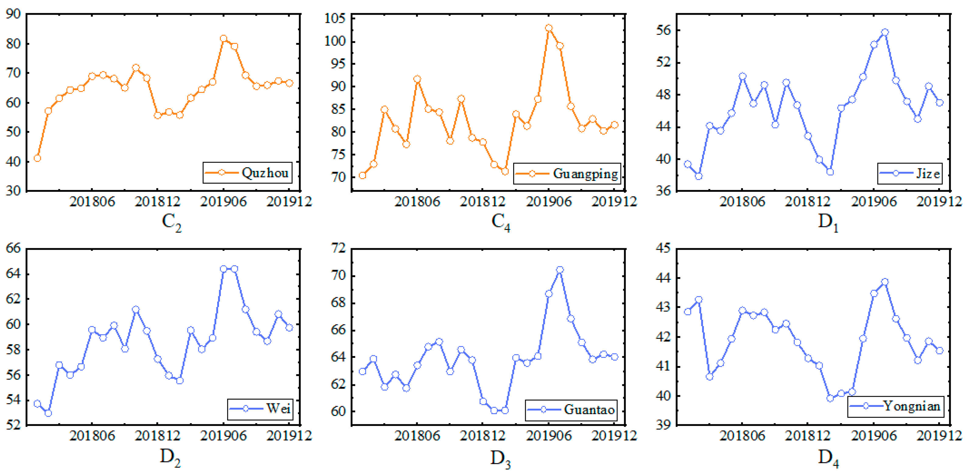
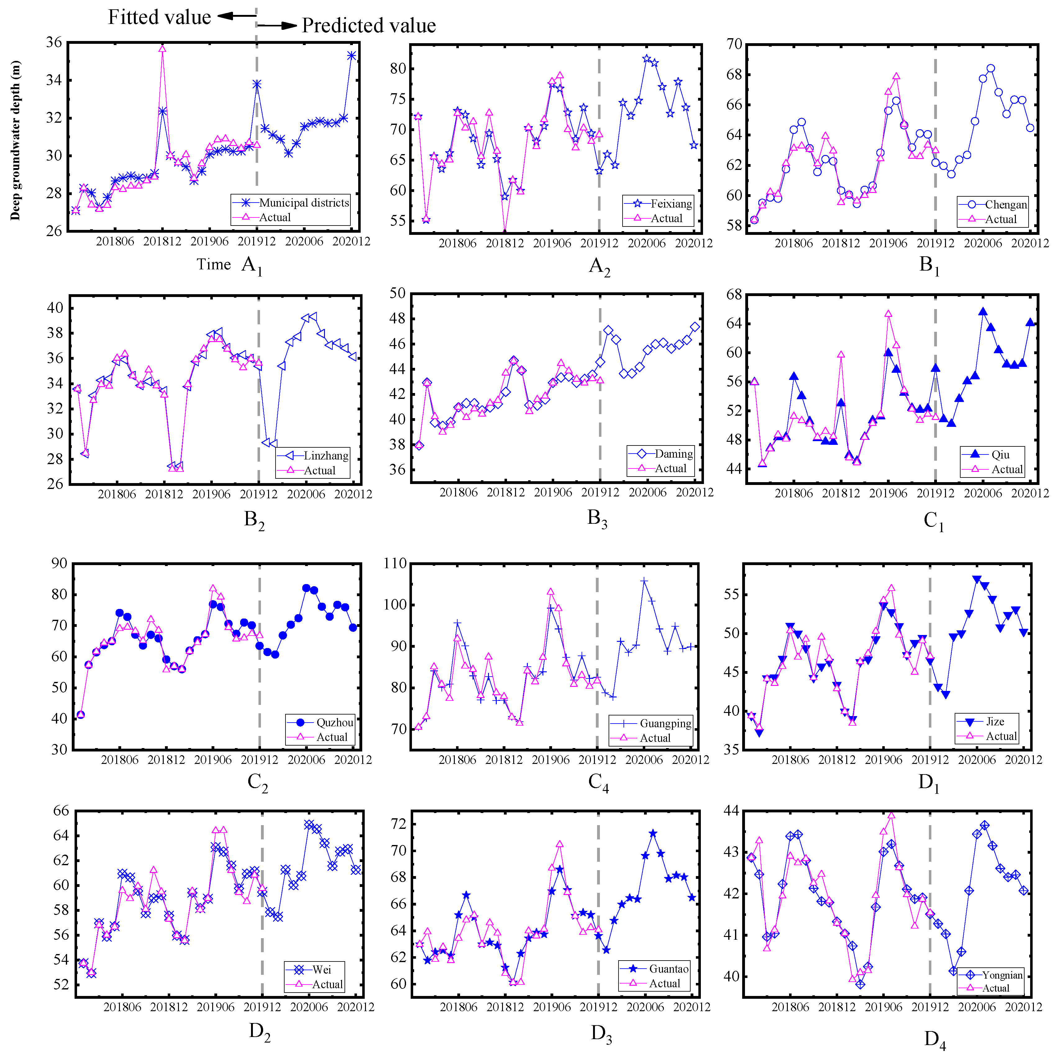
4.2. Prediction of Deep Groundwater in Handan

The acquisition cost of deep groundwater monitoring data is greater than that of shallow groundwater. Deep groundwater is also less of a concern than shallow groundwater. However, due to rapid economic development in China in recent years, people have begun to pay attention to the health of drinking water. Deep groundwater is undoubtedly the least polluted. The data on deep groundwater in Handan in the last two years is shown in Figure 5.
Due to equipment failure, the data on deep groundwater depth in Ci (C3) County is missing. By intuitive comparison with Figure 3, the seasonal fluctuation of deep groundwater is greater. The overall law is that the depth of deep groundwater appears to fall in winter. Municipal districts (A1) and Qiu County (C1) saw rapid growth in the depth of deep groundwater deposits in December 2018.
As shown in Figure 5, the variation rules of deep groundwater in various regions of Handan are not very similar, and each region has its own variation rules of deep groundwater. The modelling process is similar to that of shallow groundwater, the optimal order of the FDGSM(1,1) model in the fitting process is obtained by PSO. The values of the estimated parameters P ^ = α ^ , β ^ v are listed in Table 5. Each set of parameters is substituted into the time response Equation (13), after the restore calculation of Equation (7), the fitting data of deep groundwater depth is obtained.
The fitting and prediction results of deep groundwater depth in Handan are summarized in Table 6. From the deep groundwater depth fitting data in Table 6, Equations (16)–(18) is used to evaluate the fitting effect of the FDGSM(1,1) model. The MAPEs of each region in Handan are listed in Table 7. As shown, the error of deep groundwater is generally lower than that of shallow groundwater. The maximum error for deep groundwater is only 3.05%, but shallow groundwater is 6.73%. The comparison of the fitting error between deep and shallow groundwater depth indicates that the FGSM(1,1) model is more suitable to deal with a time series with large seasonal fluctuation. Obviously, the fluctuation of deep groundwater is more significant.
The fitting error of deep groundwater is within the allowable range. In order to further understand the variation in deep groundwater, the FDGSM(1,1) model was employed to predict the depth of deep groundwater in the next period. The predicted results are shown in Table 7. The visual results of Table 7 are shown in Figure 6. As shown, seasonal fluctuation changes are retained in the predicted results, which are consistent with the prediction characteristics of shallow groundwater. However, in the next period, the depth of deep groundwater is on the rise in all areas of Handan.

4.3. Discussion

Based on the modelling analysis of shallow and deep groundwater in Handan, the following conclusions can be determined. The shallow groundwater depth in Handan will show a small increase or maintain a stable level in the next year. It can be seen that the government’s policy of preventing and controlling overexploitation of groundwater has been effective. The pressure of shallow groundwater has been alleviated, which effectively protects the ecological environment and the water used by residents.
However, the situation in the deep groundwater is not encouraging. Deep groundwater will continue to grow in the coming year, and the growth rate is large. The reasons can be regarded as follows: On the one hand, deep groundwater is more difficult to observe and attracts less public attention than shallow groundwater. Due to the lack of public supervision, the deep groundwater treatment process is slow. On the other hand, the quality of deep groundwater is less polluted than that of shallow groundwater. Therefore, the deep groundwater consumption market is larger. Moreover, deep groundwater is more stealthily exploited, making it easier for factories to evade government regulation.
In order to alleviate groundwater pressure, the following suggestions can be taken as reference. Firstly, the government should maintain the groundwater monitoring equipment in time to ensure that the status of groundwater is understood in real time. Secondly, sewage treatment technology should be introduced to improve the utilization rate of water resources. Thirdly, sponge cities should be built to promote water circulation. Finally, in areas with serious groundwater deficiency, underground wells should be closed, and ecological water replenishment should be carried out.

5. Conclusions

In this study, the FDGSM(1,1) model is proposed to solve the problem of short-term prediction of groundwater depth. The proposed model is validated in the constructed Handan groundwater application scenario. The main findings are summarized as follows:
(1)
The fractional-order accumulation operator is effective in reducing seasonal fluctuations in groundwater data. Data fluctuations are a major source of error in seasonal forecasting. The fractional-order accumulation operator gives relief from data series fluctuations. And the heuristic algorithm searches for the optimal parameters, which improves the data processing capability of the fractional order accumulation operator.
(2)
The introduction of seasonal parameters gives seasonality to the grey prediction model. Seasonal variables are derived from the training set and can reflect the cyclical characteristics of the study population. It is found through the proof of the nature of the FDGSM(1,1) model that the proposed model maintains the basic advantages of the traditional grey forecasting model and the new model is stable and seasonal.
(3)
The predictive performance of the proposed model is validated in the Handan groundwater scenario. In this paper, a fully realistic short-term prediction scenario of groundwater depth is provided, and seasonal prediction of groundwater at different depths is accomplished based on the proposed model. The validation results show that the prediction error of the proposed model is within a reasonable interval and exhibits excellent prediction performance.
In the future, the proposed model can be attempted to be applied to more short-term groundwater predictions. Further accurately capturing the periodic variation characteristics of the data series is a direction for future improvement.

Author Contributions

Conceptualization, C.H.; supervision, K.Y.; validation, W.Y.; writing—original draft, K.Z.; writing—review and editing, L.W. All authors have read and agreed to the published version of the manuscript.

Funding

The relevant research is supported by National Social Science Found General Projects of China (grant no.23BGL031); Natural Science Foundation Youth Program of Shandong, China (grant no. ZR2023QG040); China Postdoctoral Science Foundation General project (grant no.2023M742051); National Social Science Foundation of China (21CJY055); Hebei Natural Science Foundation (E2024402142); the Hebei Graduate Student Innovation Funding Project of China(CXZZBS2025182).

Data Availability Statement

Hebei Provincial Department of Water Resources. 2024. Report on Monitoring of Groundwater Level in Groundwater Overexploitation Area of Hebei Province. Available online: http://slt.hebei.gov.cn/dynamic/search.jsp (accessed on 7 December 2024).

Conflicts of Interest

The authors declare no conflict of interest.

References

  1. Famiglietti, J.S. The global groundwater crisis. Nat. Clim. Change 2014, 4, 945–948. [Google Scholar] [CrossRef]
  2. Rodell, M.; Famiglietti, J.S.; Wiese, D.N.; Reager, J.T.; Beaudoing, H.K.; Landerer, F.W.; Lo, M.H. Emerging trends in global freshwater availability. Nature 2018, 557, 651–659. [Google Scholar] [CrossRef] [PubMed]
  3. Wada, Y. Modeling groundwater depletion at regional and global scales: Present state and future prospects. Surv. Geophys. 2016, 37, 419–451. [Google Scholar] [CrossRef]
  4. Jasechko, S.; Perrone, D.; Befus, K.M.; Cardenas, M.B.; Ferguson, G.; Gleeson, T.; Luijendijk, E.; McDonnell, J.J.; Taylor, R.G.; Wada, Y.; et al. Global aquifers dominated by fossil groundwaters but wells vulnerable to modern contamination. Nat. Geosci. 2017, 10, 425–429. [Google Scholar] [CrossRef]
  5. Gorelick, S.M.; Zheng, C. Global change and the groundwater management challenge. Water Resour. Res. 2015, 51, 3031–3051. [Google Scholar] [CrossRef]
  6. Castellazzi, P.; Martel, R.; Rivera, A.; Huang, J.; Pavlic, G.; Calderhead, A.I.; Chaussard, E.; Garfias, J.; Salas, J. Groundwater depletion in Central Mexico: Use of GRACE and InSAR to support water resources management. Water Resour. Res. 2016, 52, 5985–6003. [Google Scholar] [CrossRef]
  7. Chen, J.; Wu, H.; Qian, H.; Li, X. Challenges and prospects of sustainable groundwater management in an agricultural plain along the Silk Road Economic Belt, north-west China. Int. J. Water Resour. Dev. 2018, 34, 354–368. [Google Scholar] [CrossRef]
  8. Thomas, B.F.; Famiglietti, J.S. Sustainable groundwater management in the arid Southwestern US: Coachella Valley, California. Water Resour. Manag. 2015, 29, 4411–4426. [Google Scholar] [CrossRef]
  9. Davis, K.F.; Rulli, M.C.; Seveso, A.; D’Odorico, P. Increased food production and reduced water use through optimized crop distribution. Nat. Geosci. 2017, 10, 919–924. [Google Scholar] [CrossRef]
  10. Fishman, R.; Devineni, N.; Raman, S. Can improved agricultural water use efficiency save India’s groundwater? Environ. Res. Lett. 2015, 10, 084022. [Google Scholar] [CrossRef]
  11. Anderson, R.G.; Lo, M.; Swenson, S.; Famiglietti, J.S.; Tang, Q.; Skaggs, T.H.; Lin, Y.H.; Wu, R.J. Using satellite-based estimates of evapotranspiration and groundwater changes to determine anthropogenic water fluxes in land surface models. Geosci. Model Dev. 2015, 8, 3021–3031. [Google Scholar] [CrossRef]
  12. Machiwal, D.; Jha, M.K.; Singh, V.P.; Mohan, C. Assessment and mapping of groundwater vulnerability to pollution: Current status and challenges. Earth-Sci. Rev. 2018, 185, 901–927. [Google Scholar] [CrossRef]
  13. Jia, X.; O’Connor, D.; Hou, D.; Jin, Y.; Li, G.; Zheng, C.; Ok, Y.S.; Tsang, D.C.; Luo, J. Groundwater depletion and contamination: Spatial distribution of groundwater resources sustainability in China. Sci. Total Environ. 2019, 672, 551–562. [Google Scholar] [CrossRef] [PubMed]
  14. Hunink, J.E.; Contreras, S.; Soto-García, M.; Martin-Gorriz, B.; Martinez-Álvarez, V.; Baille, A. Estimating groundwater use patterns of perennial and seasonal crops in a Mediterranean irrigation scheme, using remote sensing. Agric. Water Manag. 2015, 162, 47–56. [Google Scholar] [CrossRef]
  15. Russo, T.A.; Lall, U. Depletion and response of deep groundwater to climate-induced pumping variability. Nat. Geosci. 2017, 10, 105–108. [Google Scholar] [CrossRef]
  16. Singh, A.; Krause, P.; Panda, S.N.; Flugel, W. Rising water table: A threat to sustainable agriculture in an irrigated semi-arid region of Haryana, India. Agric. Water Manag. 2010, 97, 1443–1451. [Google Scholar] [CrossRef]
  17. Béjar-Pizarro, M.; Guardiola-Albert, C.; García-Cárdenas, R.P.; Herrera, G.; Barra, A.; López Molina, A.; Tessitore, S.; Staller, A.; Ortega-Becerril, J.A.; García-García, R.P. Interpolation of GPS and geological data using InSAR deformation maps: Method and application to land subsidence in the alto guadalentín aquifer (SE Spain). Remote Sens. 2016, 8, 965. [Google Scholar] [CrossRef]
  18. Moosavi, V.; Vafakhah, M.; Shirmohammadi, B.; Behnia, N. A wavelet-ANFIS hybrid model for groundwater level forecasting for different prediction periods. Water Resour. Manag. 2013, 27, 1301–1321. [Google Scholar] [CrossRef]
  19. Chen, W.; Panahi, M.; Khosravi, K.; Pourghasemi, H.R.; Rezaie, F.; Parvinnezhad, D. Spatial prediction of groundwater potentiality using ANFIS ensembled with teaching-learning-based and biogeography-based optimization. J. Hydrol. 2019, 572, 435–448. [Google Scholar] [CrossRef]
  20. Chang, F.; Chang, L.; Huang, C.; Kao, I. Prediction of monthly regional groundwater levels through hybrid soft-computing techniques. J. Hydrol. 2016, 541, 965–976. [Google Scholar] [CrossRef]
  21. Suryanarayana, C.; Sudheer, C.; Mahammood, V.; Panigrahi, B.K. An integrated wavelet-support vector machine for groundwater level prediction in Visakhapatnam, India. Neurocomputing 2014, 145, 324–335. [Google Scholar] [CrossRef]
  22. Chitsazan, N.; Tsai, F.T.C. A hierarchical Bayesian model averaging framework for groundwater prediction under uncertainty. Groundwater 2015, 53, 305–316. [Google Scholar] [CrossRef] [PubMed]
  23. Deng, J. Introduction to grey system theory. J. Grey Syst. 1989, 1, 1–24. [Google Scholar]
  24. Wu, L.; Liu, S.; Yao, L.; Yan, S.; Liu, D. Grey system model with the fractional order accumulation. Commun. Nonlinear Sci. Numer. Simul. 2013, 18, 1775–1785. [Google Scholar] [CrossRef]
  25. Liu, L.; Liu, S.; Fang, Z.; Jiang, A.; Shang, G. The recursive grey model and its application. Appl. Math. Model. 2023, 119, 447–464. [Google Scholar] [CrossRef]
  26. Bahrami, S.; Hooshmand, R.; Parastegari, M. Short term electric load forecasting by wavelet transform and grey model improved by PSO (particle swarm optimization) algorithm. Energy 2014, 72, 434–442. [Google Scholar] [CrossRef]
  27. Wu, L.; Liu, S.; Liu, D.; Fang, Z.; Xu, H. Modelling and forecasting CO2 emissions in the BRICS (Brazil, Russia, India, China, and South Africa) countries using a novel multi-variable grey model. Energy 2015, 79, 489–495. [Google Scholar] [CrossRef]
  28. Ma, X.; Deng, Y.; Ma, M. A novel kernel ridge grey system model with generalized Morlet wavelet and its application in forecasting natural gas production and consumption. Energy 2024, 287, 129630. [Google Scholar] [CrossRef]
  29. Yang, W.; Hao, M.; Hao, Y. Innovative ensemble system based on mixed frequency modeling for wind speed point and interval forecasting. Inf. Sci. 2023, 622, 560–586. [Google Scholar] [CrossRef]
  30. Hao, Y.; Wang, X.; Wang, J.; Yang, W. A new perspective of wind speed forecasting: Multi-objective and model selection-based ensemble interval-valued wind speed forecasting system. Energy Convers. Manag. 2024, 299, 117868. [Google Scholar] [CrossRef]
  31. Wang, X.; Wang, L.; An, W. Probability density prediction for carbon allowance prices based on TS2Vec and distribution Transformer. Energy Econ. 2024, 140, 107986. [Google Scholar] [CrossRef]
  32. Xie, N.M.; Liu, S.F. Discrete GM (1, 1) and mechanism of grey forecasting model. Syst. Eng.-Theory Pract. 2005, 1, 93–99. [Google Scholar]
  33. Wu, L.; Liu, S.; Yao, L.; Yan, S. The effect of sample size on the grey system model. Appl. Math. Model. 2013, 37, 6577–6583. [Google Scholar] [CrossRef]
  34. Tseng, F.Y.H.; Tzeng, G. Applied hybrid grey model to forecast seasonal time series. Technol. Forecast. Soc. Change 2001, 67, 291–302. [Google Scholar] [CrossRef]
  35. Xia, M.; Wong, W.K. A seasonal discrete grey forecasting model for fashion retailing. Knowl.-Based Syst. 2014, 57, 119–126. [Google Scholar] [CrossRef]
  36. Wang, Z.; Li, Q.; Pei, L. A seasonal GM (1, 1) model for forecasting the electricity consumption of the primary economic sectors. Energy 2018, 154, 522–534. [Google Scholar] [CrossRef]
  37. Wu, L.F.; Li, N.; Zhao, T. Using the seasonal FGM (1, 1) model to predict the air quality indicators in Xingtai and Handan. Environ. Sci. Pollut. Res. 2019, 26, 14683–14688. [Google Scholar] [CrossRef]
  38. Zhou, W.; Ding, S. A novel discrete grey seasonal model and its applications. Commun. Nonlinear Sci. Numer. Simul. 2021, 93, 105493. [Google Scholar] [CrossRef]
  39. Hebei Provincial Department of Water Resources. Report on Monitoring of Groundwater Level in Groundwater Overexploitation Area of Hebei Province. 2024. Available online: http://slt.hebei.gov.cn/dynamic/search.jsp (accessed on 7 December 2024).
  40. Wu, L.; Liu, S.; Fang, Z.; Xu, H. Properties of the GM (1, 1) with fractional order accumulation. Appl. Math. Comput. 2015, 252, 287–293. [Google Scholar] [CrossRef]
  41. Wu, L.; Liu, S.; Cui, W.; Liu, D.; Yao, T. Non-homogenous discrete grey model with fractional-order accumulation. Neural Comput. Appl. 2014, 25, 1215–1221. [Google Scholar] [CrossRef]
  42. Wu, L.; Liu, S.; Yao, L. Discrete grey model based on fractional order accumulate. Syst. Eng.-Theory Pract. 2014, 34, 1822–1827. [Google Scholar]
  43. Salhein, K.; Kobus, C.J.; Zohdy, M. Forecasting Installation Capacity for the Top 10 Countries Utilizing Geothermal Energy by 2030. Thermo 2022, 2, 334–351. [Google Scholar] [CrossRef]
Figure 1. Administrative district map of Handan.
Fractalfract 09 00117 g001
Figure 2. Flowchart of the FDGSM(1,1) model based on particle swarm optimization algorithm.
Fractalfract 09 00117 g002
Figure 3. Shallow groundwater depth in various areas of Handan.
Fractalfract 09 00117 g003
Figure 4. Prediction results of shallow groundwater depth in Handan.
Fractalfract 09 00117 g004
Figure 5. Deep groundwater depth in Handan.
Fractalfract 09 00117 g005aFractalfract 09 00117 g005b
Figure 6. Forecasted results of deep groundwater depth in Handan.
Fractalfract 09 00117 g006
Table 1. Descriptive statistics of the groundwater depth data in Handan.
Statistical IndicatorsShallow GroundwaterDeep Groundwater
Average value26.8653.77
Standard error0.380.65
Median value27.1753.82
Standard deviation1.873.17
Variance3.5110.02
Kurtosis−0.261.14
Skewness−0.540.74
Minimum value23.1648.88
Maximum values29.9561.40
Sum644.721290.36
Number of observations2424
Table 2. The estimated parameters of FDGSM(1,1) model for shallow groundwater.
NumberCounty and DistrictThe Optimal Order Number Parameters   P ^ = α ^ , β ^ v
A1Municipal districts0.99 α ^ = 1.00, β ^ = [8.78, 8.49, 16.77, 15.39, 16.89, 17.55, 18.03, 16.39, 15.84, 15.82, 16.23, 10.65].
A2Feixiang1.05 α ^ = 1.01, β ^ = [33.36, 32.58, 48.77, 49.57, 53.24, 58.35, 56.54, 53.15, 51.19, 52.6, 52.5, 40.11].
B1Chengan1.02 α ^ = 1.00, β ^ = [48.85, 47.98, 49.49, 47.42, 49.76, 52.58, 51.73, 49.07, 47.84, 49.4, 48.96, 49.18].
B2Linzhang1.05 α ^ = 1.01, β ^ = [39.35, 40.08, 41.35, 40.16, 41.49, 43.59, 44.61, 41.18, 39.92, 40.51, 40.51, 38.97].
B3Daming1.05 α ^ = 1.01, β ^ = [27.23, 27.08, 28.02, 26.92, 27.03, 28.33, 27.66, 27.25, 26.93, 28.72, 27.44, 27.74].
C1Qiu1.05 α ^ = 1.01, β ^ = [12.39, 13.03, 13.82, 13.51, 13.54, 14.85, 14.4, 13.54, 12.98, 13.21, 13.13, 12.76].
C2Quzhou1.2 α ^ = 1.02, β ^ = [16.85, 16.35, 18.12, 18.08, 18.47, 19.51, 19.98, 19.78, 18.73, 19.7, 19.03, 17.93].
C3Ci1.06 α ^ = 1.02, β ^ = [5.24, 5.24, 7.24, 6.87, 7.33, 8.59, 8.2, 7.4, 7.24, 7.06, 7.57, 6.23].
C4Guangping1.03 α ^ = 1.01, β ^ = [23.36, 23.36, 25.81, 24.07, 24.51, 26.59, 26.69, 25, 24.21, 25.89, 25.46, 24.79].
D1Jize0.98 α ^ = 1.00, β ^ = [31.46, 30.28, 35.71, 31.88, 33.16, 34.5, 33.32, 31.12, 29.59, 31.45, 32.16, 28.11].
D2Wei0.99 α ^ = 1.00, β ^ = [32.24, 32.12, 34.82, 29.71, 30.61, 32.44, 32.54, 29.84, 29.13, 31.8, 30.08, 28.66].
D3Guantao1.02 α ^ = 1.00, β ^ = [22.52, 23.26, 25.27, 23.07, 23.05, 25.01, 24.6, 23.78, 22.99, 24.17, 23.52, 22.82.
D4Yongnian1.06 α ^ = 1.01, β ^ = [24.83, 23.87, 27.89, 26.02, 26.6, 28.04, 27.42, 27.56, 26.02, 26.68, 27.37, 27.48].
Table 3. Evaluation results of the FDGSM(1,1) model in each county (shallow groundwater).
NumberCounty and DistrictMAPEMAERMSE
A1Municipal districts6.73%0.941.48
A2Feixiang4.63%1.943.24
B1Chengan1.10%0.530.66
B2Linzhang1.50%0.590.78
B3Daming0.58%0.150.18
C1Qiu1.74%0.230.34
C2Quzhou2.40%0.340.48
C3Ci2.70%0.200.33
C4Guangping1.55%0.390.52
D1Jize2.62%0.911.17
D2Wei2.51%0.851.19
D3Guantao1.48%0.350.44
D4Yongnian2.41%0.600.73
Table 4. The fitted and predicted values of shallow groundwater depth in the counties and districts of Handan (unit: m).
DateABCD
Municipal DistrictsFeixiangChenganLinzhangDamingQiuQuzhouCiGuangpingJizeWeiGuantaoYongnian
Fitted value
Jan-201811.9125.8847.7138.9525.3612.0813.704.6133.9221.2725.8816.3726.53
Feb-20188.6631.4847.1738.4325.9812.5213.895.0531.0822.9331.4823.0132.45
Mar-201817.0046.9748.3539.0226.4313.0514.336.9736.9024.7946.9726.2835.42
Apr-201815.8146.7646.0937.4425.0312.5913.366.4933.5022.5046.7623.8430.54
May-201817.4349.9748.3638.6325.0312.5613.306.9535.0322.4949.9724.2331.57
Jun-201818.2154.7151.1140.6026.2613.8314.028.2336.6524.4654.7125.5133.54
Jul-201818.8152.5350.1941.5025.5013.3114.147.8235.7424.0652.5324.7333.78
Aug-201817.3049.0947.5438.0225.1012.4413.707.0833.7623.2749.0924.8331.22
Sep-201816.8447.3046.3736.9324.8311.9312.607.0232.4022.5347.3023.2630.61
Oct-201816.9048.9248.0137.7126.6812.2213.756.9434.3923.7948.9224.0133.38
Nov-201817.4048.9347.6137.8325.3912.1813.017.5635.3023.1748.9324.7231.79
Dec-201811.9236.7147.9036.4425.7911.8512.076.2931.4622.5536.7124.8430.46
Jan-201910.0630.6647.6437.0425.3511.5411.315.4534.9022.3330.6622.2334.12
Feb-20199.7830.5646.8537.9525.3112.2611.195.6133.9223.1430.5621.4634.14
Mar-201918.0847.2248.4539.3726.3713.0713.307.7339.5125.2247.2225.6636.95
Apr-201916.8647.6746.4538.3125.3312.7713.187.3835.9723.0647.6723.7031.99
May-201918.4651.3548.9139.8625.5812.8613.687.9337.3923.1451.3524.4232.96
Jun-201919.2356.4351.8042.1027.0014.2314.809.2838.9325.1856.4325.9334.88
Jul-201919.8254.5250.9943.2226.4013.7815.238.9337.9624.8254.5225.3335.10
Aug-201918.2951.3048.4239.9326.1212.9715.048.2535.9324.0851.3025.5632.51
Sep-201917.8349.7047.3338.9925.9412.5014.168.2434.5323.3949.7024.1231.88
Oct-201917.8951.4849.0339.9027.8812.8315.508.2036.4924.6751.4824.9734.63
Nov-201918.3951.6348.6840.1426.6712.8314.928.8737.3724.0951.6325.7633.02
Dec-201912.9039.5449.0238.8527.1312.5414.137.6433.5023.4839.5425.9631.68
Predicted value
Jan-202011.0433.6148.8039.55 26.7612.2613.51 6.8424.0936.9235.3323.2923.42
Feb-202010.7633.6148.0540.54 26.7713.0013.52 7.0324.2535.9335.3524.1322.72
Mar-202019.0650.3749.6942.05 27.8813.8415.76 9.1926.8541.5138.1526.2226.97
Apr-202017.8350.9147.7241.05 26.8913.5715.75 8.8825.1837.9533.1824.0825.07
May-202019.4354.6750.2142.67 27.1913.6816.36 9.4625.7739.3634.1424.1725.83
Jun-202020.2059.8353.1244.99 28.6515.0617.59 10.8527.9840.8936.0626.2327.38
Jul-202020.7958.0052.3446.17 28.0814.6318.12 10.5428.1639.9136.2725.8926.82
Aug-202019.2754.8549.8042.93 27.8413.8418.04 9.8826.5837.8733.6825.1627.10
Sep-202018.8153.3248.7342.04 27.7013.3917.26 9.9125.9536.4733.0524.4825.69
Oct-202018.8755.1750.4543.01 29.6713.7418.69 9.9127.8038.4335.7925.7826.58
Nov-202019.3755.3850.1243.31 28.4913.7518.22 10.6127.4739.3034.1925.2027.40
Dec-202013.8843.3550.4842.07 28.9813.4717.53 9.4226.9435.4332.8524.6127.64
Table 5. The estimated parameters of FDGSM(1,1) model for deep groundwater.
NumberCounty and DistrictThe Optimal Order Number Parameters   P ^ = α ^ , β ^ v
A1Municipal districts1 α ^ = 1.00, β ^ = [28.64, 28.17, 27.82, 26.96, 27.35, 28.13, 28.18, 28.16, 27.93, 27.82, 27.95, 31.13].
A2Feixiang0.99 α ^ = 1.00, β ^ = [56.26, 54.15, 64.16, 61.52, 63.69, 70.2, 69.01, 64.67, 59.95, 64.86, 60.23, 53.74].
B1Chengan1.02 α ^ = 1.00, β ^ = [61.22, 60.47, 61.23, 61.36, 63.4, 66.06, 66.62, 64.86, 63.21, 63.94, 63.71, 61.66].
B2Linzhang0.16 α ^ = 0.96, β ^ = [−3.22, 1.57, 8.24, 5.33, 3.97, 4.87, 3.69, 2.13, 2.23, 3.17, 2.7, 2.35].
B3Daming1.02 α ^ = 1.01, β ^ = [44.41, 43.47, 40.54, 40.28, 40.55, 41.66, 41.9, 41.78, 41.08, 41.17, 41.28, 42.07].
C1Qiu1.06 α ^ = 1.01, β ^ = [48.83, 47.42, 50.2, 52.17, 52.47, 60.82, 58.57, 55.02, 52.39, 51.51, 51.11, 56.05].
C2Quzhou1.05 α ^ = 1.01, β ^ = [60.59, 59.07, 64.58, 67.72, 69.49, 78.88, 78.08, 72.48, 68.65, 71.73, 70.44, 63.33].
C4Guangping1.05 α ^ = 1.01, β ^ = [77.56, 75.71, 88.39, 85.56, 86.81, 101.78, 96.94, 89.66, 83.43, 88.44, 82.47, 81.99].
D1Jize1.02 α ^ = 1.01, β ^ = [39.13, 37.86, 44.88, 45.09, 47.46, 51.62, 50.54, 48.49, 44.44, 45.66, 46.03, 42.84].
D2Wei0.99 α ^ = 1.00, β ^ = [52.77, 52.29, 55.95, 54.53, 55.12, 59.1, 58.55, 57.25, 55.26, 56.3, 56.34, 54.53].
D3Guantao1.02 α ^ = 1.00, β ^ = [60.8, 62.77, 63.76, 64.04, 63.71, 66.74, 68.23, 66.51, 64.37, 64.34, 63.95, 62.14].
D4Yongnian1.03 α ^ = 1.00, β ^ = [43.97, 43.66, 42.71, 43.1, 44.52, 45.87, 46.09, 45.57, 44.98, 44.7, 44.7, 44.25].
Table 6. The fitted and predicted values of deep groundwater depth in the counties and districts of Handan (unit: m).
DateABCD
Municipal DistrictsFeixiangChenganLinzhangDamingQiuQuzhouGuangpingJizeWeiGuantaoYongnian
Fitted value
Jan-201827.1072.1558.3833.5837.9555.9341.3670.5239.4253.7462.9942.87
Feb-201828.2855.2059.5128.4542.9344.6557.3472.7637.3352.9461.7742.47
Mar-201828.0465.6459.8733.0539.7646.8461.4584.1044.2556.9662.4140.96
Apr-201827.3063.5659.8034.2639.4948.3763.7680.1044.3655.8862.5241.04
May-201827.7966.1661.7534.4139.8048.3965.0280.9646.7756.7262.1442.23
Jun-201828.6873.1164.3535.7840.9856.6574.1295.7051.0160.9465.1943.39
Jul-201828.8472.4464.8735.9041.3054.0272.8390.1950.0060.6566.6843.43
Aug-201828.9468.5463.1234.6441.2950.5567.1482.9448.1159.5765.0142.80
Sep-201828.8264.1961.5533.8640.7248.2363.5977.1444.2957.7862.9842.13
Oct-201828.8369.4162.4034.1740.9647.7567.0582.7245.7858.9863.1341.82
Nov-201829.0765.1862.2733.9441.2447.7265.9276.9646.3859.2162.8941.79
Dec-201832.3759.0060.3333.4442.1953.0259.1177.0543.4157.5861.2541.33
Jan-201930.0161.7660.0627.4744.6945.9056.9773.0939.9855.9760.1141.04
Feb-201929.6659.9659.4527.4643.8945.1155.9971.8639.0255.6262.2840.74
Mar-201929.4370.2560.3733.7741.1448.4161.9985.1346.3259.4163.4439.81
Apr-201928.6968.0560.6435.7741.1250.6965.3382.2746.6858.1963.8840.24
May-201929.1970.5762.8336.3241.6051.2667.2883.9349.2758.9363.7441.68
Jun-201930.0877.4665.6237.8942.9159.9576.8899.2753.6563.0766.9643.01
Jul-201930.2576.7466.2738.1043.3457.6576.0094.2352.7662.7368.6043.20
Aug-201930.3672.8264.6536.8643.4254.4770.6487.3850.9761.6067.0542.68
Sep-201930.2468.4463.1836.0442.9252.4067.3681.9147.2359.7665.1342.11
Oct-201930.2573.6464.1136.3043.2352.1471.0687.7848.8060.9465.3541.87
Nov-201930.5069.4064.0435.9943.5652.3170.1482.2849.4661.1465.1941.91
Dec-201933.8163.2162.1735.3944.5757.7963.5282.5946.5659.4863.6241.51
Predicted value
Jan-202031.4565.9661.9629.3247.1150.8461.5478.8443.1857.8562.5541.28
Feb-202031.1164.1661.4029.2146.3650.1960.7277.8042.2757.4964.7741.03
Mar-202030.8874.4562.3735.4043.6553.6466.8791.2549.6261.2765.9840.14
Apr-202030.1472.2562.6837.3043.6656.0570.3488.5650.0360.0366.4740.60
May-202030.6574.7764.9137.7544.1856.7572.4190.3652.6760.7666.3742.07
Jun-202031.5581.6767.7439.2145.5365.5682.13105.8557.0964.8969.6343.44
Jul-202031.7280.9568.4339.3245.9963.3981.36100.9556.2464.5471.3143.65
Aug-202031.8477.0366.8337.9746.0960.3276.1094.2354.4963.4069.7943.16
Sep-202031.7372.6665.3937.0645.6358.3772.9388.8950.7961.5667.9042.61
Oct-202031.7577.8766.3537.2345.9658.2276.7394.8852.4062.7368.1642.40
Nov-202032.0073.6466.3136.8246.3258.4975.9189.5053.0962.9268.0342.46
Dec-202035.3167.4664.4736.1447.3664.0869.3889.9250.2361.2666.4942.08
Table 7. Evaluation results of the FDGSM(1,1) model in each county (Deep groundwater).
DateABCD
Municipal DistrictsFeixiangChenganLinzhangDamingQiuQuzhouGuangpingJizeWeiGuantaoYongnian
MAPE1.90%2.56%1.06%0.92%1.10%3.05%2.90%2.48%2.17%1.00%1.35%0.73%
MAE0.591.720.730.410.471.742.222.171.060.650.90.39
RMSE1.032.380.870.560.622.672.742.71.540.971.230.55
Disclaimer/Publisher’s Note: The statements, opinions and data contained in all publications are solely those of the individual author(s) and contributor(s) and not of MDPI and/or the editor(s). MDPI and/or the editor(s) disclaim responsibility for any injury to people or property resulting from any ideas, methods, instructions or products referred to in the content.

