Direct Synthesis of Fractional-Order Controllers Using Only Two Design Equations with Robustness to Parametric Uncertainties

Abstract

This paper employs the Direct Synthesis approach to present an analytical methodology for designing fractional-order controllers, aiming to balance simplicity and robustness for practical industrial implementation. Although significant progress has been made in developing fractional-order PID controllers, the advancement of Direct Synthesis controllers has been comparatively slower. This study underscores the importance of further research on these controllers and the need for innovative approaches to enhance parameter adjustment. The proposed methodology is based on the fractional “second-order” transfer function and the solution of two equations derived from four key specifications: overshoot, settling time, and the frequency and magnitude of disturbance rejection. Additionally, the fractional order should be chosen as close as possible to 1, ensuring practical implementation and minimizing the system’s sensitivity to parameter variations. The resulting controller demonstrates strong robustness against plant parameter variations, input noise, and disturbances while achieving shorter settling times and lower overshoot. It outperforms fractional-order PID and ID controllers optimized numerically and surpasses integer-order phase lead-lag compensators designed analytically. The validation process involved Monte Carlo simulations and Kruskal–Wallis statistical analysis on a complex system characterized by closely spaced poles and significant parametric variations. Furthermore, the proposed controller effectively reduces the integral of the control signal (control effort), enhancing energy efficiency.

1. Introduction

Fractional calculus is a mathematical framework that involves derivatives and integrals of non-integer order. One of its main uses is in the accurate modeling and robust design of intricate systems. The use of fractional control in the design of Fractional-Order Controllers (FOCs) is of particular interest. Experimental research indicates that FOCs are less susceptible to variations in plant parameters and provide superior performance in terms of reaction characteristics, including settling time, overshoot, and disturbance rejection, when compared to Integer-Order Controllers (IOCs). However, to the best of the authors’ knowledge, there is currently no formal proof to substantiate this assertion. However, its use is widely acknowledged, resulting in four regularly used types of FOCs in process control: Oustaloup’s CRONE controller [1], Podlubny’s fractional-order Proportional-Integral-Derivative controller (FOPID) [2] (with variants such as the FO Integral-Derivative controller (FOID) [3]), the fractional-order lead-lag compensator [4], and Chen’s fractional-order phase shaper [5]. Subsequently, several authors have proposed various FOCs derived from those previously mentioned. Nevertheless, the problem of improving the parameters of FOCs remains challenging in the field of control engineering. Various suggestions have been examined, including analytical methodology [6], numerical techniques [7], and rule-based methods [8], most of which were initially designed for controllers with integer order. Additional methods that can be employed include adaptive control [9], fractional-order Ziegler–Nichols methods [8], neural networks [10], genetic algorithms [11], metaheuristics [12], Monje’s techniques [13], and performance index minimization [11].

FOPID and FOID controllers offer greater flexibility than their integer-order counterparts by introducing adjustable orders, allowing them to meet multiple specifications, enhance robustness against uncertainties, and optimize the balance between stability, settling time, and disturbance rejection [13]. They provide more precise, smooth, and efficient control, making them ideal for complex systems. The FOPID controller, by including proportional action, improves disturbance rejection and accuracy compared to the FOID controller. Both are typically tuned through optimization by solving nonlinear equations, but the FOID benefits from approximate formulas derived from these processes, simplifying its design [3]. However, tuning parameters and hardware implementation pose significant challenges for the fractional-order PID controller (FOPID), which is widely discussed in the literature as the most extensively studied FOC [7,8,9,10,11,12,13,14,15,16,17,18,19,20,21].

Unfortunately, in comparison to FOPID controllers, there is a noticeable lag in the development of FOCs through the Direct Synthesis (DS) approach [20,21,22,23,24,25]. DS is a method that is frequently employed in IOCs and provides a simple approach: the controller structure is directly aligned with the desired closed-loop transfer function. The primary benefit of DS is that the closed-loop system closely resembles the desired system, which enables control of the system’s dynamics by adjusting the desired characteristics. The DS approach necessitates an explicit process model, which is one of its drawbacks.

Among the few reported works on FOC using the DS technique, the following can be found. An FOC was presented in [22] to regulate systems having one or two poles characterized by fractional orders, in addition to an integer first-order reference. However, there was no reference to stability studies or instructions for modifying the controller parameters. In [24], the authors examined a procedure using a fractional-order pole as the plant with a fractional “second-order” transfer function as the benchmark. The reference parameters were determined using a genetic algorithm to guarantee the desired closed-loop step response, which includes optimization of the Integrated Square Error (ISE). In [25], the desired closed-loop transfer function was selected as Bode’s ideal loop transfer function. However, this technique was limited to achieving a desired response of first-order and relied on empirical calculations that took into account peak overshoot and settling time. In [7], a DS approach was used to control a process with an integer-order plus delay. However, rather than relying on a mathematical model, they adjusted the controller using time-domain inputs to achieve optimal performance.

Another alternative that incorporates DS is the Internal Model Controller (IMC). In an IMC, the controller is designed to continuously compare the output of the real process with the output of the model [23]. If there is a discrepancy between the two, it indicates the presence of disturbances that the controller must rectify. This method often utilizes Bode shaping in the frequency domain and incorporates an internal process model into the controller [18]. This enables the controller to predict the system’s reactions to various control operations. Here, the DS approach commonly involves modifying a single parameter in order to accomplish a trade-off between system performance and its tolerance to variations [26,27]. However, its execution necessitates meticulous calibration. In a similar way, the study described in [20] offered a DS technique using a Smith predictor structure to develop a controller that integrates a cascaded FOPID controller with a fractional-order filter. This approach relies on time-domain specifications and Bode’s ideal transfer function to attain the intended closed-loop response. It considers a first-order plus reference model and provides approximate analytical expressions for overshoot and settling time.

These recent studies highlight the ongoing, yet still nascent, research on the design of FOCs using the DS approach (FO-DS). Excluding IMC-based implementations, which predominantly focus on FOPID controllers, there are relatively few investigations into FO-DS. Thus, we emphasize the need to further explore this method and develop innovative strategies to tune its parameters. To achieve this objective, this work seeks to develop an analytical method for designing FO-DS controllers that balance simplicity and robustness for practical industrial implementation. The proposed approach requires solving only two equations based on four key specifications: overshoot, settling time, and frequency and magnitude of disturbance rejection. Furthermore, the fractional order should be chosen as close as possible to 1, ensuring practical implementation and minimizing the system’s sensitivity to parameter variations. The resulting controllers should be robust to variations in plant parameters and demonstrate effectiveness in lowering the integrated squared error and the integrated control signal, hence promoting energy efficiency.

The block diagram depicted in Figure 1 shows the controlled system intended for evaluating the suggested methodology. The input signal will consist of a unit step function with 10% white noise, and the disturbance will be a unit step applied at t = 2500 s. A Monte Carlo study will be performed to simulate parameter variability. The suggested controller is going to be evaluated against other controllers, such as the FOPID controller, the integer-order phase lead-lag compensator, and the fractional-order Integral Derivative controller. The main focus of the comparison will be on their effectiveness in handling disturbances, noise, and parameter variability.

The findings of this study highlight the advantages of the proposed fractional-order Direct Synthesis (FO-DS) controller, which provides a simple and analytical design approach based on only four specifications, two equations, and guidelines for selecting the fractional order. The FO-DS controller surpasses fractional-order PID, fractional-order ID, and integer-order lead-lag compensators by achieving lower overshoot, shorter settling time, and reduced control effort. One of the key benefits of this approach is its remarkable improvement in energy efficiency, reducing the integrated control signal effort by over 90% compared to the fractional PID controller. Monte Carlo simulations and statistical analysis confirm the robustness and effectiveness of the proposed method, demonstrating its ability to handle parametric uncertainties and disturbances. Furthermore, the simplicity of the FO-DS controller design streamlines its practical implementation without the need for complex numerical optimization methods, positioning it as an efficient and viable solution for industrial applications.

This work is structured as follows: Section 2 covers the theoretical foundation, including the canonical second-order transfer function, fractional calculus, the three-term fractional-order transfer function, the integer-order lead-lag compensator, fractional-order PID and ID controllers, Direct Synthesis control, and performance metrics like the Integrated Square Error (ISE) and Integral Square Control Error Performance Index (ISCE), along with Monte Carlo analysis, the Lilliefors normality test, and Levene’s test. Section 3 introduces the proposed Direct Synthesis method. Section 4 illustrates the method with an example applied to controlling steam pressure in the upper dome of a bagasse boiler. In Section 5, simulation results compare the proposed method with FOPID, integer lead-lag, and fractional-order Integral Derivative controllers. Section 6 discusses the results and Section 7 presents the conclusions.

2. Theoretical Background

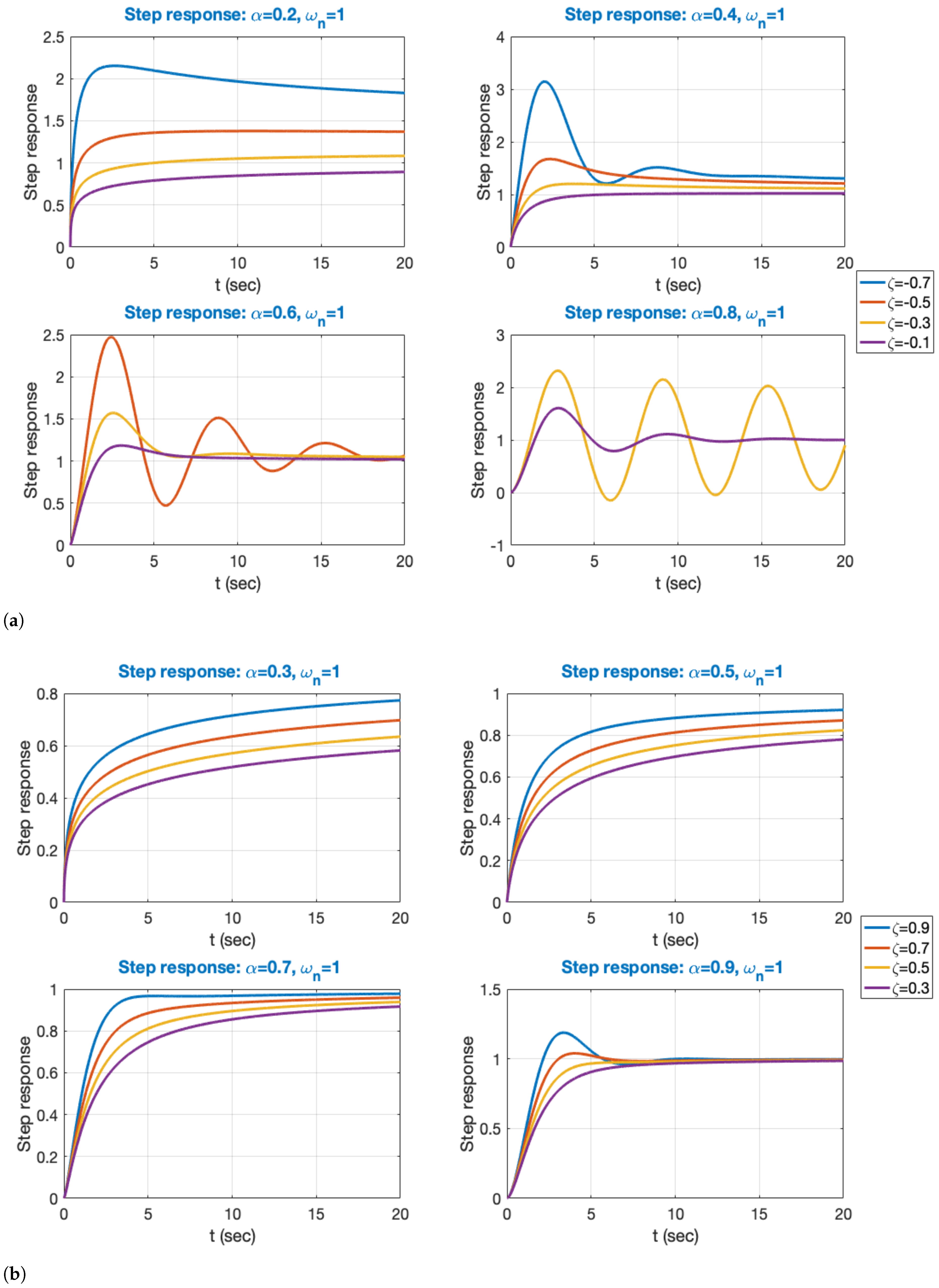
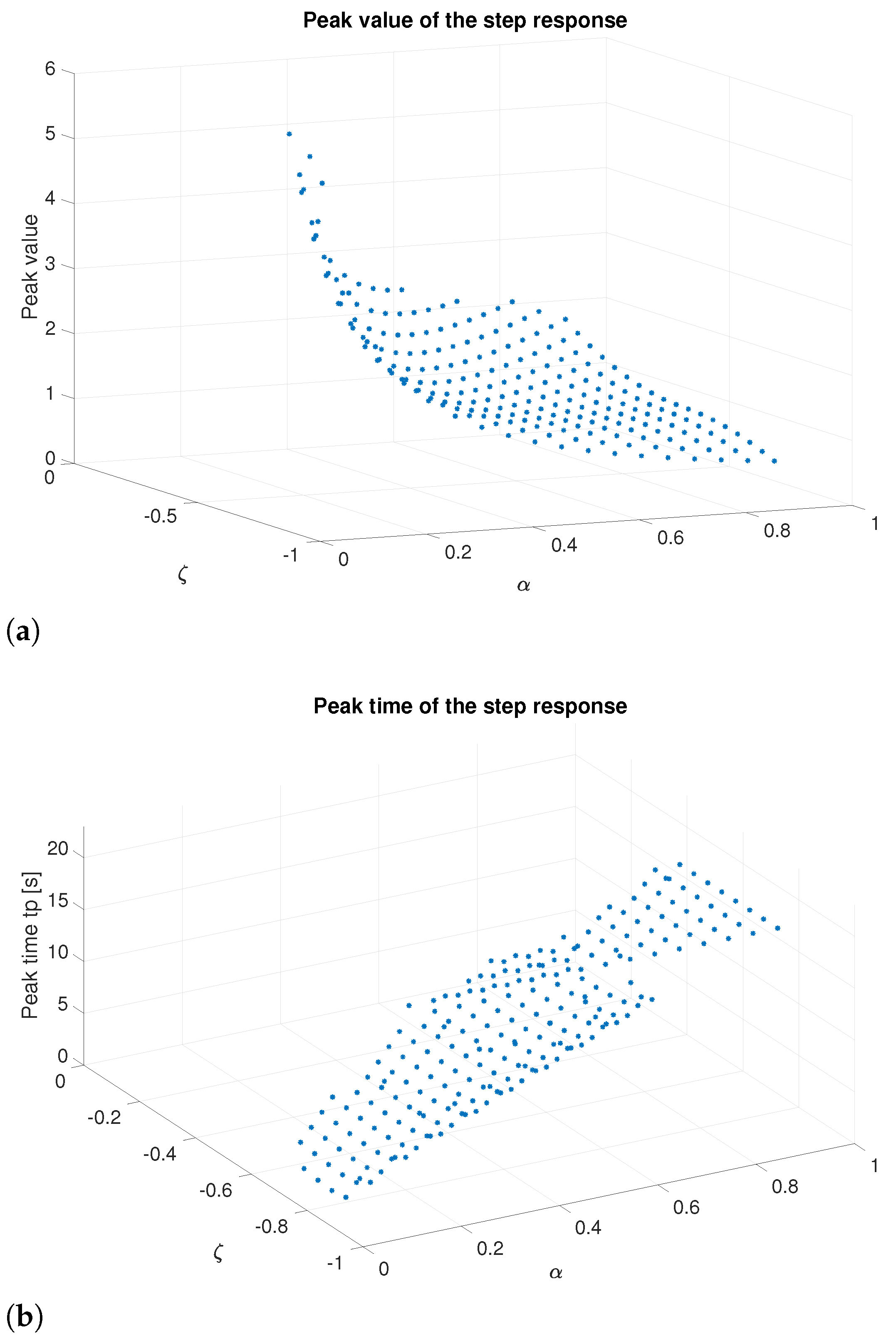
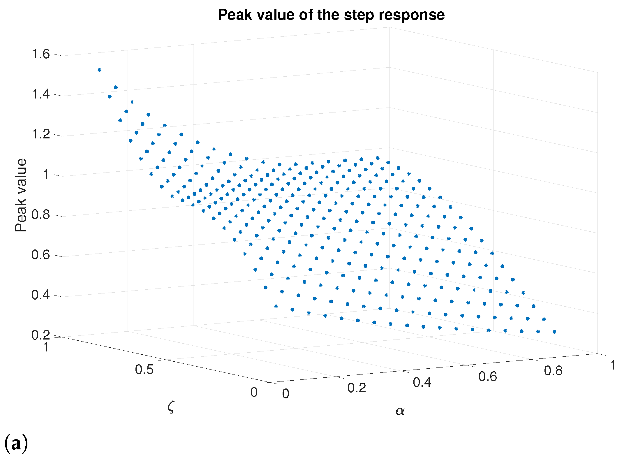
2.1. Second-Order Canonical Transfer Function

The transfer function of a second-order underdamped canonical system can be represented by through:

$$G_{CL}\left(s\right)={\displaystyle \frac{{\omega }_c^2}{s^2+2\xi {\omega }_{c}s+{\omega }_c^2}},0<\xi <1,$$

(1)

where $\xi$ represents the damping factor, while ${\omega }_c$ specifies the undamped natural frequency of the system. The condition $0<\xi <1$ guarantees that the system remains underdamped. An underdamped system exhibits oscillatory behavior with exponential decay, which is essential in many control applications to ensure both stability and responsiveness. We will use the representation ${\omega }_c$ in the integer-order version of (1) and ${\omega }_n$ in its fractional-order version (see (13)), as both parameters will be essential for the calculations involved in the design of controllers through Direct Synthesis. The step response and frequency response characteristics of (1) are interrelated by the following expressions [28]:

$$\xi = \left|-ln\left({\displaystyle \frac{M_p}{100}}\right){\left[{\pi }^2+{ln}^2\left({\displaystyle \frac{M_p}{100}}\right)\right]}^{-0.5}\right|,$$

(2)

$$\begin{array}{ccc}\hfill {\varphi }_m& =& arctan\left(2\xi {\left[-2{\xi }^2+\sqrt{4{\xi }^4+1}\right]}^{-0.5}\right)\hfill \\ & \approx & 100\xi ,\mathrm{if}\xi <0.7,\hfill \end{array}$$

(3)

$$\begin{array}{ccc}\hfill {\omega }_c& =& {\displaystyle \frac{4}{\xi t_s}}\sqrt[]{(1-2{\xi }^2)+\sqrt[]{4{\xi }^4-4{\xi }^2+2}}\hfill \\ & \approx & {\displaystyle \frac{4}{\xi t_s}}\approx {\displaystyle \frac{400}{{\varphi }_m{t}_s}}\mathrm{if}\xi <0.7,\hfill \end{array}$$

(4)

$$\begin{array}{ccc}\hfill e_{ss}& =& {\displaystyle \frac{100\%}{1+{10}^{\frac{M_l}{20}}},}\hfill \end{array}$$

(5)

$$\begin{array}{ccc}\hfill K_n& =& {\displaystyle {10}^{\frac{M_l}{20}}=\frac{100}{e_{ss}}-1,}\hfill \end{array}$$

(6)

where the symbol $M_p$ represents the required overshoot, ${\varphi }_m$ represents the phase margin, $t_s$ denotes the settling time of 2%, and $M_l$ and $K_n$ correspond to the loop gain in decibels and magnitude, respectively. The importance of these parameters, $M_l$ and $K_n$, lies in their function of attaining the appropriate steady-state error, $e_{ss}$, for a ramp input signal.

2.2. Fractional Calculus

Fractional calculus generalizes differentiation and integration, denoted by the operator ${}_a\mathrm{D}_t^{\alpha }$, where a and t represent the operator’s limits. The definition of this operator is as follows, with $\alpha$ showing the order of the operation [29]:

$${}_a\mathrm{D}_t^{\alpha }=\left\{\begin{array}{cc}{\displaystyle \frac{{\mathrm{d}}^{\alpha }}{\mathrm{d}{t}^{\alpha }}}\hfill & \mathrm{if}\Re \left(\alpha \right)>0\hfill \\ 1\hfill & \mathrm{if}\Re \left(\alpha \right)=0\hfill \\ {\int }_a^t{\left(d\tau \right)}^{-\alpha }\hfill & \mathrm{if}\Re \left(\alpha \right)<0\hfill \end{array}\right.$$

(7)

Among the definitions for the operator ${}_a\mathrm{D}_t^{\alpha }$, the Riemann–Liouville definition is notable. As stated in [30]:

$${\displaystyle {\mathrm{D}}_t^{\alpha }f\left(t\right)={\displaystyle \frac{1}{\mathsf{\Gamma }(n-\alpha )}}{\displaystyle \frac{d^n}{d{t}^n}}{\int }_0^t{(t-\tau )}^{n-\alpha -1}f\left(\tau \right)d\tau },$$

(8)

where n is an integer such that $n-1<\alpha <n$, and $\mathsf{\Gamma }\left(x\right)$ is the Euler Gamma function:

$$\mathsf{\Gamma }\left(x\right)={\int }_0^{\infty }{t}^{x-1}{e}^{-t}dt,\mathrm{Re}\left(x\right)>0.$$

(9)

If we denote the Laplace transform of $f\left(t\right)$ as $F\left(s\right)$, then we can express the Laplace transform of (8) with initial conditions set to zero as follows:

$$\mathcal{L}\left\{{}_{a}D_t^{\alpha }f\left(t\right)\right\}=s^{\pm \alpha }F\left(s\right),$$

(10)

with

$$s^{\alpha }={\omega }^{\alpha }cos\left({\displaystyle \frac{\alpha \pi }{2}}\right)+j{\omega }^{\alpha }sin\left({\displaystyle \frac{\alpha \pi }{2}}\right),$$

(11)

which can be approximated over a range of frequencies (${\omega }_l$, ${\omega }_h$) with an nth-order Oustaloup filter [24,31]:

$$\begin{array}{ccc}\hfill s^{\alpha }& \approx & {\omega }_h^{\alpha }\prod _{k=1}^n{\displaystyle \frac{s+{\omega }_k^{\prime }}{s+{\omega }_k}},\hfill \\ \hfill {\omega }_k^{\prime }& =& {\omega }_l{\left({\displaystyle \frac{{\omega }_h}{{\omega }_l}}\right)}^{(2k-1-\alpha )/2n},\hfill \\ \hfill {\omega }_k& =& {\omega }_l{\left({\displaystyle \frac{{\omega }_h}{{\omega }_l}}\right)}^{(2k-1+\alpha )/2n}.\hfill \end{array}$$

(12)

In this work, the Riemann–Liouville definition is used due to its suitability for frequency-domain analysis, as its Laplace transform directly expresses fractional derivatives in terms of the operator $s^{\alpha }$. Additionally, since initial conditions are assumed to be zero, no further reformulation is required. Furthermore, the Riemann–Liouville definition is more commonly used than the Caputo or other definitions in studies focused on frequency-domain methods. However, the Caputo definition could be useful if a clearer physical interpretation is needed or if working with nonzero initial conditions is anticipated [32].

2.3. Three-Term Fractional-Order Canonical Form

The definition of the three-term fractional-order transfer function is as follows: [33]:

$$G_{CLf}\left(s\right)={\displaystyle \frac{{\omega }_n^2}{s^{2\alpha }+2\zeta {\omega }_n{s}^{\alpha }+{\omega }_n^2}}.$$

(13)

In this formulation, $\alpha$∈$(0,2)$ denotes the fractional order, and ${\omega }_n$ $>>$ 0 along with $\zeta$ are real parameters. Matignon’s theorem states that the stability of (13) does not depend on ${\omega }_n$, allowing for negative values of $\zeta$ provided that [24,33]:

$$\zeta >-cos\left({\displaystyle \frac{\alpha \pi }{2}}\right).$$

(14)

Figure 2a illustrates the step responses of (13) with ${\omega }_n = 1$, while varying $\alpha$ and $\zeta$ within the ranges of (0.2, 0.8) and (−0.7, −0.1) in increments of 0.2, when the stability condition (13) is met (Matlab™  simulation with fifth-order Oustaloup approximation). For smaller values of $\alpha$, the responses increase. However, as $\zeta$ becomes more negative, the underdamped responses exhibit a greater overshoot. The number of overshoots rises with $\alpha$, whereas the number of stable cases diminishes. Figure 2b illustrates the step responses of (13) with ${\omega }_n$ = 1, while $\alpha$ and $\zeta$ vary within the ranges of $(0.3, 0.9)$. For $\alpha$ values below 0.5, the responses increase. As $\alpha$ rises, underdamped responses and overshoot increase with $\zeta$. These responses differ from typical second-order systems, as the number of overshoots depends on $\alpha$. An increase in ${\omega }_n$ leads to a reduction in settling time. However, to limit significant overshoots, it is advisable to adjust the value of $\alpha$ to enhance speed [33]. According to Figure 3, for negative $\zeta$ values, the peak value decreases and $t_p$ increases as $\zeta$ becomes more negative. This trend is observed as $\alpha$ increases. For positive $\zeta$ values (Figure 4), the peak value decreases, and $t_p$ increases as $\zeta$ decreases. A similar trend is noticeable as $\alpha$ increases; however, a significant change in $t_p$ behavior is clear only when $\alpha$ exceeds 0.5.

2.4. Controllers

2.4.1. Integer-Order Phase Lead/Lag Compensator

Phase lag compensation reduces steady-state error by increasing the system’s gain and adjusting the phase margin to achieve the desired percentage overshoot. Phase lead compensation reduces overshoot and increases bandwidth, thus speeding up the transient response. In (15), $K_c$ represents the required gain to meet $e_{ss}$, while M (in decibels) and p (in radians, $-\pi /2\le p\le \pi /2$) denote the gain and phase that the compensator should provide at the frequency $\omega$ = ${\omega }_c$ to attain the desired values of $M_p$ and $t_s$. The compensator reported in [34,35] accomplishes these goals using:

$$\begin{array}{ccc}\hfill C_{LL}\left(s\right)& =& K_c\left({\displaystyle \frac{1+\alpha \tau s}{1+\tau s}}\right),\hfill \\ \hfill \alpha & =& {\displaystyle \frac{d(d\sqrt{1+{\delta }^2}-1)}{d-\sqrt{1+{\delta }^2}}}\tau ={\displaystyle \frac{d-\sqrt{1+{\delta }^2}}{d\delta {\omega }_c}},\hfill \\ \hfill d& =& {10}^{M/20},\delta =tan\left(p\right).\hfill \end{array}$$

(15)

2.4.2. Fractional-Order PID Controller

We can extend PID controllers to fractional order, where $K_p$, $K_i$, and $K_d$ denote the proportional, integral, and derivative gains, and $\mu$ and $\lambda$∈$(0,2)$ the order of the differentiator and integrator. The representation of these controllers is [2,36]:

$$C_{PIDf}\left(s\right)=K_p+{\displaystyle \frac{K_i}{s^{\lambda }}}+K_d{s}^{\mu }=K_p\left(1+{\displaystyle \frac{1}{T_i{s}^{\lambda }}}+T_d{s}^{\mu }\right).$$

(16)

The fractional $PID$ controller has enhanced flexibility, which arises from incorporating fractional powers. As a result, this controller structure allows tuning of five parameters ($\lambda$, $\mu$, $K_p$, $K_i$, and $K_d$). The fractional orders can effectively fulfill additional design specifications, including rejecting noise, perturbations, and constraints on the gain margin $M_g$, making them suitable for robust control.

2.4.3. Fractional-Order ID Controller

The $I{D}^{\alpha -1}$ controller is a fractional-order variant of the PID controller that includes an integral term of integer order and a fractional-order differentiator. In the Laplace domain, this controller results in [3]:

$$C_{I{D}^{\alpha -1}}\left(s\right)={\displaystyle \frac{K_i}{s}}+K_d{s}^{\alpha -1}.$$

(17)

The order $\alpha$ is used to maximize robustness against changes in the plant gain. The design procedure involves sweeping $\alpha$ in the range (0, 2) and obtaining different values of $K_i$ and $K_d$ using equations similar to (24) (phase margin), but without explicit knowledge of the loop gain $L\left(j{\omega }_c\right)$. Once each controller has been computed, the phase crossover frequency ${\omega }_s$ and the gain margin $M_g$ are numerically determined. The optimization is concluded by selecting the transfer function with the highest gain margin.

2.4.4. Fractional-Order Direct Synthesis Control

Direct Synthesis (DS) is a common strategy in control theory. If $G_p\left(s\right)$ is the system model and $G_{CLf}\left(s\right)$ is the predetermined fractional-order closed-loop transfer function to achieve the desired response, then the controller results in [7]:

$$C_{DS}\left(s\right)={\displaystyle \frac{1}{G_p\left(s\right)}}\left[{\displaystyle \frac{G_{CLf}\left(s\right)}{1-G_{CLf}\left(s\right)}}\right],$$

(18)

and for $G_{CLf}\left(s\right)$, as defined in (13), (18) yields

$$C_{DS}\left(s\right)={\displaystyle \frac{L\left(s\right)}{G_p\left(s\right)}}={\displaystyle \frac{1}{G_p\left(s\right)}}\left[{\displaystyle \frac{{\omega }_n^2}{s^{\alpha }\left(s^{\alpha }+2\zeta {\omega }_n\right)}}\right],$$

(19)

with the loop gain given by

$$L\left(s\right)={\displaystyle \frac{{\omega }_n^2}{s^{\alpha }\left(s^{\alpha }+2\zeta {\omega }_n\right)}}.$$

(20)

2.5. Performance Metrics and Statistical Analysis

Beyond the usual performance measures, such as settling time, steady-state error, and overshoot, we will incorporate additional indices and analyses into our evaluation.

2.5.1. Integrated Square Error (ISE)

The error signal, $e\left(t\right)=r\left(t\right)-y\left(t\right)$, represents the difference between the reference signal $r\left(t\right)$ (setpoint) and the controlled signal $y\left(t\right)$. When evaluating controller performance, it is a common practice to employ the integrated square error (ISE) as a performance metric. It provides a measure of performing of a control system in minimizing the error between the desired and actual responses. The following formula is used to compute the ISE over a time interval, from an instant $t_i$ to an instant $t_f$ ($T=t_f-t_i$) [37,38]:

$$\begin{array}{c}\hfill {\displaystyle ISE={\int }_{t_i}^{t_f}e{\left(t\right)}^{2}dt.}\end{array}$$

(21)

It is also possible to use a normalized version of (21), given by $IS{E}_n$ = $ISE/(t_f-t_i)$.

2.5.2. Integral Square Control Error Performance Index (ISCE)

This index weighs the minimization of the control action. We define it as as the sum of the integral of the square of the error and the integral of the square of the control action $u\left(t\right)$ [37]:

$$\begin{array}{c}\hfill ISC{E}_n={\displaystyle \frac{{\displaystyle {\int }_{t_i}^{t_f}e{\left(t\right)}^{2}dt+{\int }_{t_i}^{t_f}u{\left(t\right)}^{2}dt}}{t_f-t_i}}.\end{array}$$

(22)

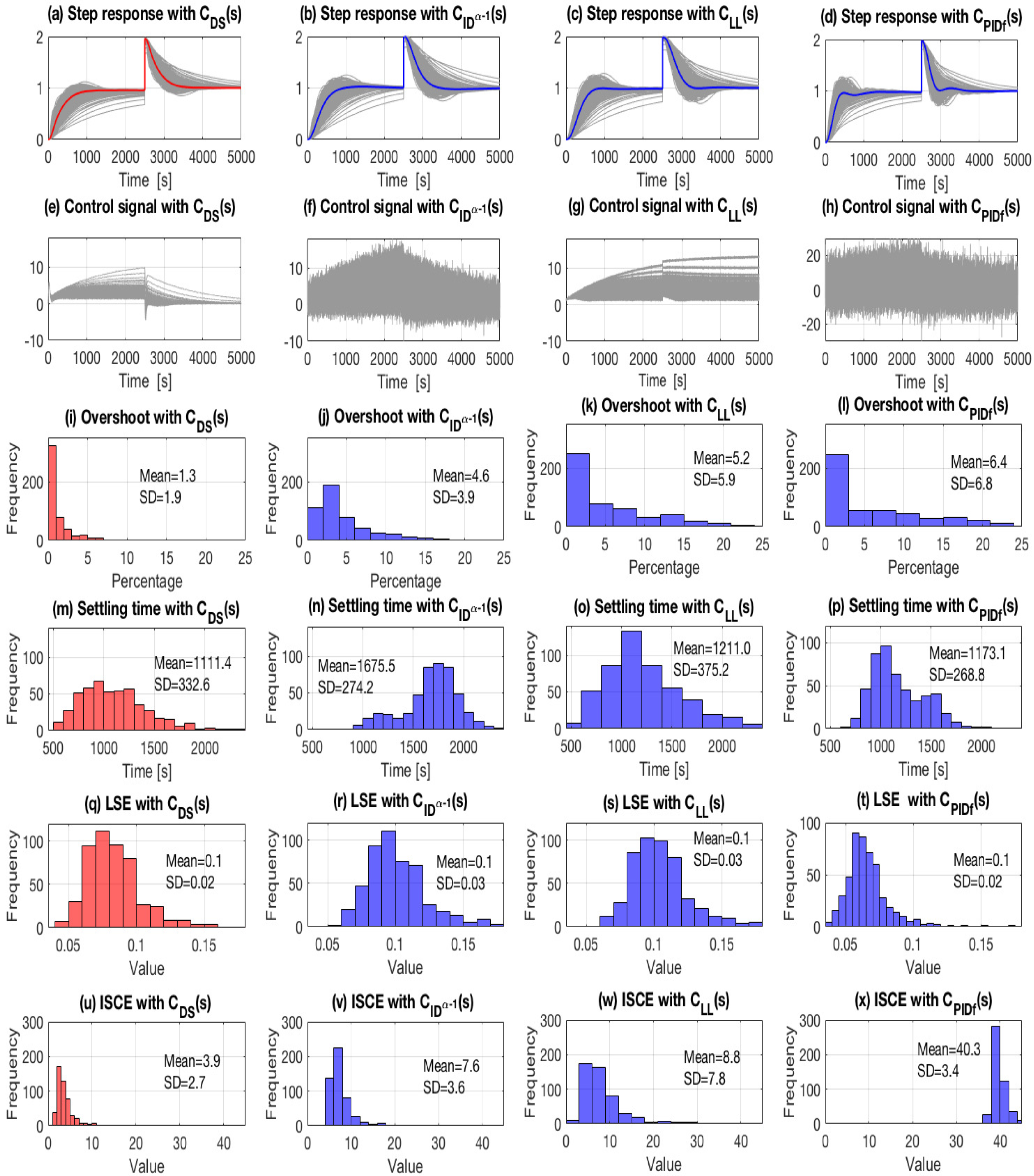
2.5.3. Monte Carlo Analysis

It is a computational method used to assess the impact of uncertainty and variability in a system or model, such as in PID controllers [39]. This method involves simulating many scenarios, derived from the probability distributions of uncertain variables, and subsequent recording of outcomes for each of these scenarios. For instance, to simulate four hundred cases of plant gain variation in Matlab, adopting a normal distribution with a nominal value of $K_p$ = 1 and a standard deviation making up 25%, we employ the following code:

• % MonteCarlo Analysis
• % Parameter variations and normal distribution
• Kp = 1;             % nominal gain
• N = 400;           % number of cases
• des = 0.25;       % 25% std deviation
• % Gain variation
• Kp_mc = normrnd(Kp, des∗Kp).

2.5.4. Lilliefors Normality Test

The test compares the empirical cumulative distribution of data with the expected cumulative distribution of a normal distribution [40]. If the p-value is very low (usually < 0.05), the null hypothesis of normality is rejected. Researchers use this method in statistical analysis to verify assumptions of normality, which are crucial in procedures such as analysis of variance. It involves comparing the empirical cumulative distribution of the data with the expected cumulative distribution of a normal distribution. If the p-value is low (<0.05), we reject the null hypothesis of normality, which suggests that the data do not follow a normal distribution.

2.5.5. Levene’s Test

The homoscedasticity (equal variances) among groups can be evaluated using Levene’s test [41]. It can be used instead of Bartlett’s test of variance and is less affected by changes from normality.

2.5.6. Kruskal–Wallis Test

The Kruskal–Wallis test is a statistical technique that is employed to compare the medians of three or more independent datasets. It is not a parametric test, which means it does not need assumptions of normality or homoscedasticity (equal values), unlike the analysis of variance [42]. If the p-value is lower than a particular significance level (for example, 0.05), this shows that there are significant differences between the levels of the medians. Subsequently, a post hoc multiple comparisons test is employed to determine which groups exhibit significant disparities in their medians and establish confidence ranges.

3. Proposed Method

To develop the proposed method, we will start by considering the system depicted in Figure 1, with $G_{CLf}\left(s\right)$ and $L\left(s\right)$ given by (13) and (20), and with the controllers (15)–(17) and (19). We will derive expressions to calculate the phase margin, gain margin, response to disturbances at the output, and the phase crossover frequency ${\omega }_s$. The design specifications will include ${\varphi }_m$ (or $M_p$), ${\omega }_c$ (or $t_s$), ${\omega }_t$ (disturbances bandwidth) and A (gain at ${\omega }_t$). The objectives will be the optimization of the gain margin through selecting an appropriate value for $\alpha$ and setting suitable values for $\zeta$ and ${\omega }_n$ that fulfill the desired requirements. Let us assume we know the value of $\alpha$, which we will justify in the gain margin analysis. In addition, since ${\omega }_t$ is smaller than ${\omega }_c$, we will consider

$${\omega }_t=0.01\delta {\omega }_c.$$

(23)

where $\delta$ is a positive constant.

3.1. Stability Analysis

The stability analysis of the proposed method is inherently guaranteed by the closed-loop compensated system, which always adopts the form shown in Equation (13) (three-term FO canonical form). According to Matignon’s theorem, such a system is stable if ${\omega }_n$ is positive and the damping factor satisfies (14). These conditions will be explicitly considered during the design process, ensuring the stability of the system without requiring further analysis.

3.2. Phase Margin

The relationship between the phase margin ${\varphi }_m$, the gain crossover frequency ${\omega }_c$ and the loop gain $L\left(s\right)$ given by (20) can be expressed as [3]

$$L\left(j{\omega }_c\right)={\displaystyle \frac{{\omega }_n^2}{{\left(j{\omega }_c\right)}^{\alpha }\left[{\left(j{\omega }_c\right)}^{\alpha }+2\zeta {\omega }_n\right]}}=-cos{\varphi }_m-jsin{\varphi }_m,$$

(24)

By substituting (11) into (24) with $s=j{\omega }_c$, we obtain:

$$-cos{\varphi }_m={\displaystyle \frac{{\omega }_n^2\left[{\omega }_c^{2\alpha }cos\left(\alpha \pi \right)+2\zeta {\omega }_n{\omega }_c^{\alpha }cos(\alpha \pi /2)\right]}{{\omega }_c^{4\alpha }+4{\zeta }^2{\omega }_n^2{\omega }_c^{2\alpha }+4\zeta {\omega }_n{\omega }_c^{3\alpha }cos(\alpha \pi /2)}},$$

(25)

$$-sin{\varphi }_m=-{\displaystyle \frac{{\omega }_n^2\left[{\omega }_c^{2\alpha }sin\left(\alpha \pi \right)+2\zeta {\omega }_n{\omega }_c^{\alpha }sin(\alpha \pi /2)\right]}{{\omega }_c^{4\alpha }+4{\zeta }^2{\omega }_n^2{\omega }_c^{2\alpha }+4\zeta {\omega }_n{\omega }_c^{3\alpha }cos(\alpha \pi /2)}}$$

(26)

Dividing (26) by (25) results in:

$$tan{\varphi }_m=-{\displaystyle \frac{{\omega }_c^{2\alpha }sin\left(\alpha \pi \right)+2\zeta {\omega }_n{\omega }_c^{\alpha }sin(\alpha \pi /2)}{{\omega }_c^{2\alpha }cos\left(\alpha \pi \right)+2\zeta {\omega }_n{\omega }_c^{\alpha }cos(\alpha \pi /2)}}.$$

(27)

From which, we can solve for $2\zeta {\omega }_n$:

$$2\zeta {\omega }_n=-{\omega }_c^{\alpha }\left[{\displaystyle \frac{sin\left(\alpha \pi \right)+cos\left(\alpha \pi \right)tan\left({\varphi }_m\right)}{sin(\alpha \pi /2)+cos(\alpha \pi /2)tan\left({\varphi }_m\right)}}\right]$$

$$=-{\omega }_c^{\alpha }\left[{\displaystyle \frac{\sqrt{1+{tan}^2\left({\varphi }_m\right)}sin(\alpha \pi +{\varphi }_m)}{\sqrt{1+{tan}^2\left({\varphi }_m\right)}sin(\alpha \pi /2+{\varphi }_m)}}\right].$$

(28)

Resulting in the first design equation, given by:

$$2\zeta {\omega }_n=-{\omega }_c^{\alpha }\left[{\displaystyle \frac{sin(\alpha \pi +{\varphi }_m)}{sin(\alpha \pi /2+{\varphi }_m)}}\right]\approx -{\left({\displaystyle \frac{400}{{\varphi }_m{t}_s}}\right)}^{\alpha }\left[{\displaystyle \frac{sin(\alpha \pi +{\varphi }_m)}{sin(\alpha \pi /2+{\varphi }_m)}}\right],\mathrm{if}\xi <0.7.$$

(29)

Assuming that $\alpha$ has a known value in Equation (29) (subject to further analysis), and given that ${\varphi }_m$, $t_s$, and ${\omega }_c$ are design requirements, we can continue with the remaining computations by assuming a constant and known value for $2\zeta {\omega }_n$.

3.3. Disturbance Response

Suppose we have a known value for $2\zeta {\omega }_n=B$. Let us analyze the system’s response to disturbances at the frequency ${\omega }_t$ while limiting it to a gain of A. This situation corresponds to [43]:

$${\displaystyle \frac{1}{|1+L(j{w}_t\left)\right|}}=A.$$

(30)

Using the triangle inequality, we have

$$1+|L\left(j{w}_t\right)| \ge |1+L\left(j{w}_t\right)| = {\displaystyle \frac{1}{A}}.$$

(31)

Or, equivalently,

$$|L\left(j{w}_t\right)| = {\displaystyle \frac{{\omega }_n^2}{|{\left(j{\omega }_t\right)}^{\alpha }\left|\right|{\left(j{\omega }_t\right)}^{\alpha }+B|}}\ge {\displaystyle \frac{1}{A}}-1.$$

(32)

By rigorously solving this inequality for ${\omega }_n$, excluding negative solutions, and employing (23), we deduce the second design equation:

$$\begin{array}{cc}\hfill {\omega }_n& =\sqrt{\left({\displaystyle \frac{1}{A}}-1\right)}\sqrt[4]{{\omega }_t^{4\alpha }+2B{\omega }_t^{3\alpha }cos(\alpha \pi /2)+B^2{\omega }_t^{2\alpha }}\hfill \\ \hfill & \approx \sqrt{\left({\displaystyle \frac{1}{A}}-1\right)}\sqrt[4]{{\left({\displaystyle \frac{4\delta }{{\varphi }_m{t}_s}}\right)}^{4\alpha }+2B{\left({\displaystyle \frac{4\delta }{{\varphi }_m{t}_s}}\right)}^{3\alpha }cos(\alpha \pi /2)+B^2{\left({\displaystyle \frac{4\delta }{{\varphi }_m{t}_s}}\right)}^{2\alpha }}\hfill \\ \hfill & \mathrm{if}\xi <0.7.\hfill \end{array}$$

(33)

As a result, assuming a known value for $\alpha$ (and for B through the use of (29)), and considering ${\omega }_t$ and A as specifications, it becomes feasible to perform a direct computation of ${\omega }_n$.

3.4. Gain Margin

Controlling processes with dominant time delays or closely located poles presents significant challenges for automation engineers, as it can impact both phase and gain margins [43,44]. It might seem unnecessary to discuss the gain margin about expression (20); because the phase of this transfer function never becomes as negative as $-{180}^{\circ }$, it is equal to $-180\alpha$, with $\alpha$∈$(0,1)$. However, the analysis will enable us to determine the choice of $\alpha$ to reduce the system’s sensitivity to variations in its parameters.

Let ${\omega }_s$ be the frequency at which $L\left(j{\omega }_s\right)$ approaches a phase of “nearly” ${180}^{\circ }$ (i.e., ${\varphi }_m$ = 0). This “occurs” when the imaginary part of $L\left(j{\omega }_s\right)$ is equal to zero. Thus, by substituting ${\varphi }_m=0$ and replacing ${\omega }_c$ with ${\omega }_s$ in (26), we obtain:

$$-{\displaystyle \frac{{\omega }_n^2\left[{\omega }_s^{2\alpha }sin\left(\alpha \pi \right)+2\zeta {\omega }_n{\omega }_s^{\alpha }sin(\alpha \pi /2)\right]}{{\omega }^{4\alpha }+4{\zeta }^2{\omega }_n^2{\omega }_s^{2\alpha }+4\zeta {\omega }_n{\omega }_s^{3\alpha }cos(\alpha \pi /2)}}=0.$$

(34)

From which, we can solve for ${\omega }_s^{\alpha }$ to obtain

$$w_s^{\alpha }=-2\zeta {\omega }_n\left({\displaystyle \frac{sin(\alpha \pi /2)}{sin\left(\alpha \pi \right)}}\right).$$

(35)

Calculating the gain margin involves:

$$M_g={\displaystyle \frac{1}{\left|L\right(j{\omega }_s\left)\right|}}={\displaystyle \frac{|{\left(j{\omega }_s\right)}^{\alpha }\left|\right|{\left(j{\omega }_s\right)}^{\alpha }+2\zeta {\omega }_n|}{{\omega }_n^2}}$$

$$={\displaystyle \frac{|{\omega }_s^{\alpha }|}{{\omega }_n^2}}\sqrt{{\omega }_s^{2\alpha }+2\zeta {\omega }_n{\omega }_s^{\alpha }cos(\alpha \pi /2)+4{\zeta }^2{\omega }_n^2}.$$

(36)

By substituting (35) into (36), we obtain

$$\begin{array}{cc}\hfill M_g& =4{\zeta }^{2}F\left(\alpha \right)\hfill \\ \hfill =& 4{\zeta }^2\left({\displaystyle \frac{sin(\alpha \pi /2)}{sin\left(\alpha \pi \right)}}\right)\sqrt{{\left({\displaystyle \frac{sin(\alpha \pi /2)}{sin\left(\alpha \pi \right)}}\right)}^2+1.5}.\hfill \end{array}$$

(37)

As observed in Figure 5, the function $F\left(\alpha \right)$ from (37) displays an increasing behavior. Therefore, to minimize the impact of variations on the plant parameters, it is advisable to choose the highest possible value for $\alpha$ that can be implemented. But, the choice of the $\alpha$ value in the interval $(0,1)$ is constrained by the difficulties associated with implementing the $s^{\alpha }$ terms in hardware, as defined by (12). As the value of $\alpha$ approaches 1, and as n increases, the separation between the poles and zeros in (12) increases, complicating the implementation due to the appearance of poles and/or zeros at very low and very high frequencies.

3.5. Implementation Steps

• Select the largest possible values of n and $\alpha$ within the range $(0,1)$ such that hardware implementation remains practical. Typical values are often found between 3 and 6 for n, and between 0.8 and 0.95 for $\alpha$.
• Define specifications for ${\varphi }_m$ (or for $M_p$ and use (2) and (3)), ${\omega }_c$ (or for $t_s$ and use (4)), ${\omega }_t$, and A.
• Determine ${\omega }_n$ using (33).
• With this value of ${\omega }_n$, calculate $\zeta$ using (29).

4. Example

Bagasse boilers play a crucial role in the sugar cane processing industry. They convert bagasse, a byproduct of the industry, into an economical source of energy, enhancing the industry’s sustainability and cost-effectiveness. These boilers display intricate dynamic behavior, including a dominant time delay and closely located poles that present challenges in simplifying their mathematical model using conventional methods, as reported in [45]. Their dynamic parameters vary over time within wide parameter variability and are susceptible to disturbances. These boilers encompass multiple interconnected processes that must be controlled independently. In [3], a fractional-order robust control was reported to manage the steam pressure in the upper dome of a bagasse boiler, which was represented via the following mathematical model:

$$\begin{array}{cc}\hfill G_p\left(s\right)& ={\displaystyle \frac{Kexp\{-Ls\}}{(T_{1}s+1)(T_{2}s+1)}}\hfill \\ \hfill & \approx {\displaystyle \frac{K}{(T_{1}s+1)(T_{2}s+1)(Ls+1)}}\hfill \\ \hfill & ={\displaystyle \frac{0.395}{(103s+1)(93.4s+1)(120s+1)}}.\hfill \end{array}$$

(38)

Let us use the same nominal parameters as reported in [3]: $K=0.395$, $T_1=103.05$, $T_2=93.44$, and $L=120$, and design the controller based on specifications similar to those presented in [3] (see

Table 1. Design specifications.

	${\mathit{C}}_{\mathbf{DS}}\left(\mathit{s}\right)$	${\mathit{C}}_{{\mathbf{ID}}^{\mathit{\alpha }-1}}\left(\mathit{s}\right)$	${\mathit{C}}_{\mathbf{LL}}\left(\mathit{s}\right)$	${\mathit{C}}_{\mathbf{PIDf}}\left(\mathit{s}\right)$
${\varphi }_m$	64.63∘	64.63∘	64.63∘	60∘
$M_p$	5%	5%	5%	8.7%
${\omega }_c$	0.0693	0.01	0.003	0.01
$t_s$	1000 s	586 s	2000 s	586 s
A	−40 dB	-	-	−40 dB

), allowing for a comparative evaluation.

4.1. Utilization of the Method

• “Select the largest possible value of $\alpha$ within the range $(0, 1)$”: we will use $\alpha =0.9$.
• “Define specifications for ${\varphi }_m$, ${\omega }_c$, ${\omega }_t$, and A”: We will opt for specifications similar to those presented in [3]: ${\varphi }_m=61.{45}^{\circ }$, ${\omega }_c=0.0045$ rad/s, ${\omega }_t=0.000045$ rad/s and $A=-$40 dB = 0.01. Using (2)–(4) and (23) it corresponds to $M_p=5\%$, $t_s=1000$ s, and $\delta =1$.
• “Determine ${\omega }_n$ using (33)”: The resulting value of ${\omega }_n$ is 0.0143.
• “With this value of ${\omega }_n$, calculate $\zeta$ using (29)”: The value of $\zeta$ is 0.4235.

4.2. Direct Synthesis

With the calculated values of ${\omega }_n$ and $\zeta$, we obtain

$$L\left(s\right)={\displaystyle \frac{0.{0143}^2}{s^{0.9}\left[s^{0.9}+2\left(0.4235\right)\left(0.0143\right)\right]}}.$$

(39)

And with (19), (38), and (39), the controller $C_{DS}\left(s\right)$ results in:

$$C_{DS}\left(s\right)={\displaystyle \frac{(T_{1}s+1)(T_{2}s+1)(Ls+1)}{K{s}^{\alpha }}}\left({\displaystyle \frac{{\omega }_n^2}{\left[s^{\alpha }+2\xi {\omega }_n\right]}}\right)$$

(40)

$C_{DS}\left(s\right)$ is an improper fraction, which makes it non-implementable in practical systems without modifications. The most commonly adopted solution involves cascading each term of the form $\mathsf{\Theta }$s + 1 in the numerator with a first-order low-pass filter. This technique is frequently employed as a preprocessing step in data acquisition, resulting in improved system stability and noise reduction [46]. In this way, it is used as follows:

$$\mathsf{\Theta }s+1\approx {\displaystyle \frac{(1+m)\mathsf{\Theta }s+1}{m\mathsf{\Theta }s+1}},$$

(41)

where m varies between 0.1 and 1. Thus, with $m=0.1$, (40) results in

$$\begin{array}{cc}\hfill C_{DS}\left(s\right)& ={\displaystyle \frac{1}{K}}\left[{\displaystyle \frac{(1+m)T_{1}s+1}{m{T}_{1}s+1}}\right]\left[{\displaystyle \frac{(1+m)T_{2}s+1}{m{T}_{2}s+1}}\right]\left[{\displaystyle \frac{(1+m)Ls+1}{mLs+1}}\right]\left({\displaystyle \frac{{\omega }_n^2}{s^{\alpha }\left[s^{\alpha }+2\xi {\omega }_n\right]}}\right)\hfill \\ \hfill & =2.53\left({\displaystyle \frac{102.8s+1}{9.344s+1}}\right)\left({\displaystyle \frac{113.4s+1}{10.3s+1}}\right)\left({\displaystyle \frac{132s+1}{12s+1}}\right)\left({\displaystyle \frac{0.{0143}^2}{s^{0.9}\left[s^{0.9}+0.0121\right]}}\right).\hfill \end{array}$$

(42)

5. Evaluation of the Proposed Method Based on Simulations Results

Let us now compare the performance of the system depicted in Figure 1 when $G_p\left(s\right)$ follows the definition in (38) and when using the controller (42) against two other fractional-order robust controllers: the $I{D}^{\alpha -1}$ controller as computed in [3], and the $P{I}^{\alpha }{D}^{\mu }$ controller detailed in [2,36] with tuning performed using the FOMCON toolbox [47,48]. Table 1 shows the design specifications for each controller. Besides these robust control methods, we have included an integer-order control in the comparison, the phase lead-lag compensator (15) with the design specifications of Table 1. The resulting controllers are

$$\begin{array}{ccc}\hfill C_{I{D}^{\alpha -1}}\left(s\right)& =& {\displaystyle \frac{0.008525+4.9605s^{1.25}}{s}}\hfill \end{array}$$

(43)

$$\begin{array}{ccc}\hfill C_{LL}\left(s\right)& =& 251\left({\displaystyle \frac{1+\left(0.0051\right)\left(32304\right)s}{1+32304s}}\right)\hfill \end{array}$$

(44)

$$\begin{array}{ccc}\hfill C_{PIDf}\left(s\right)& =& 1.109+{\displaystyle \frac{0.024}{s^{0.9}}}+10s^{0.34}\hfill \end{array}$$

(45)

For fractional-order controllers, (12) was used to compute a fifth-order Oustaloup approximation for $s^{\pm \alpha }$ within the frequency range (${\omega }_l=0.0001$ rad/s, ${\omega }_h=100$ rad/s). We executed a Monte Carlo simulation in Matlab™, which involved 400 cases ($N=400$), to evaluate the robustness of the controllers. We defined the variations for standard deviations in the plant parameters as 25%. The reference signal included 10% white noise, and a 100% disturbance affected the output at $t=2500$ s. Figure 6 displays the simulation results. The red graphs represent the system response to the proposed control. The broader curves in Figure 6a–d depict the averaged response from the 400 analyses. Figure 6a–h show the step responses along with their corresponding control signals. Figure 6i–x showcase histograms for $M_p$, $t_s$, $IS{E}_n$, and $ISC{E}_n$.

5.1. Scenario Without Parameter Variations

Table 2. Performance metrics using the nominal parameters of $G_p\left(s\right)$. Here, $t_{per}$ and $M_{per}$ denote the time and maximum magnitude of the control signal necessary to correct the perturbation.

	${\mathit{C}}_{\mathbf{DS}}\left(\mathit{s}\right)$	${\mathit{C}}_{{\mathbf{ID}}^{\mathit{\alpha }-1}}\left(\mathit{s}\right)$	${\mathit{C}}_{\mathbf{LL}}\left(\mathit{s}\right)$	${\mathit{C}}_{\mathbf{PIDf}}\left(\mathit{s}\right)$
$M_p$	0.6%	3.7%	4%	5.5%
$t_s$	858 s	1838 s	1104 s	997 s
$IS{E}_n$	0.1	0.1	0.1	0.1
$ISC{E}_n$	3.2	4.5	6.8	12.4
$t_{per}$	857 s	832 s	650 s	640 s
$M_{per}$	5.94	18	1.78	31.17

summarizes the results in the nominal scenario (without parameter variations). All controllers meet the specifications for $M_p$ and even exceed them with respect to $t_s$, and all controllers show the ability to reject the disturbance occurring at $t=2500$ s. The $C_{DS}$ controller achieves 6.17 times lower overshoot than $C_{I{D}^{\alpha -1}}$, 6.67 times lower than $C_{LL}$, and 9.17 times lower than $C_{PIDf}$. Its settling time is 53.3% shorter than $C_{I{D}^{\alpha -1}}$, 22.3% shorter than $C_{LL}$, and 13.9% shorter than $C_{PIDf}$. In terms of $ISC{E}_n$, $C_{DS}$ performs 28.9% better than $C_{I{D}^{\alpha -1}}$, 52.9% better than $C_{LL}$, and 74.2% better than $C_{PIDf}$. However, $t_{per}$ (settling time related to the system’s response to perturbation) for $C_{DS}$ is 2.9% longer than $C_{I{D}^{\alpha -1}}$, 31.8% longer than $C_{LL}$, and 33.8% longer than $C_{PIDf}$. For $M_{per}$ (overshoot related to the system’s response to the perturbation), $C_{DS}$ achieves 33% of $C_{I{D}^{\alpha -1}}$, but is 70% higher than $C_{LL}$, and 19% of $C_{PIDf}$.

Figure 7 shows the relative values of $M_p$, $t_s$, and $ISC{E}_n$ regarding the parameter associated with the worst-performing controller, which is assigned a value of 100%. We observe significant improvements achieved by the proposed controller $C_{DS}$ under nominal conditions: up to 89.1% reduction in $M_p$ compared to the $C_{PIDf}$ control, a 53.3% decrease in $t_s$ compared to the $I{D}^{\alpha -1}$ control, and a substantial 74.2% reduction in $ISC{E}_n$ compared to the $C_{PIDf}$ control.

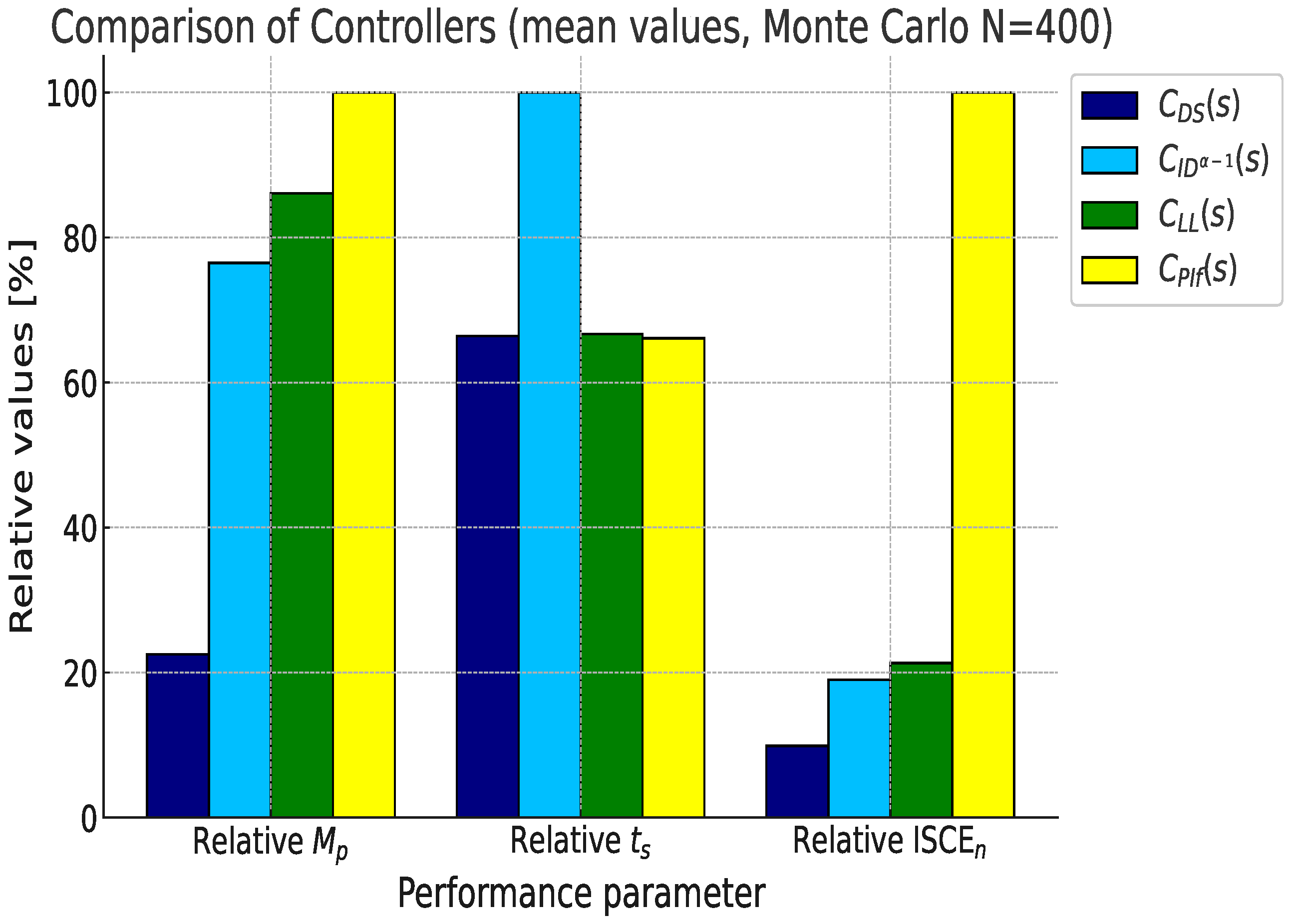
5.2. Scenario with Parameter Variations: Monte Carlo Analysis

Table 3. Performance metrics obtained considering parameter variations in $G_p\left(s\right)$ (M: mean value. SD: standard deviation).

Param	${\mathit{C}}_{\mathbf{DS}}\left(\mathit{s}\right)$	${\mathit{C}}_{{\mathbf{ID}}^{\mathit{\alpha }-1}}\left(\mathit{s}\right)$
$M_p$	M = 1.4%, SD = 1.9%	M = 4.8%, SD = 3.8%
$t_s$	M = 1116.4 s, SD = 330.2 s	M = 1660.9 s, SD = 299.2 s
$IS{E}_n$	M = 0.1, SD = 0.02	M = 0.1, SD = 0.03
$ISC{E}_n$	M = 3.9, SD = 2.2	M = 7.6, SD = 2.8
Param	${\mathbf{C}}_{\mathbf{LL}}\left(\mathbf{s}\right)$	${\mathbf{C}}_{\mathbf{PIDf}}\left(\mathbf{s}\right)$
$M_p$	M = 5.4%, SD = 5.7%	M = 6.3%, SD = 6.5%
$t_s$	M = 1224 s, SD = 361.9 s	M = 1113.4 s, SD = 244.7 s
$IS{E}_n$	M = 0.1, SD = 0.02	M = 0.1, SD = 0.02
$ISC{E}_n$	M = 8.6, SD = 5.9	M = 40.8, SD = 2.6

summarizes the results considering the parameter variations and the Monte Carlo analysis. Once again, the proposed controller outperforms the others in terms of mean values of overshoot, settling time, and control effort. Figure 8 presents the relative values of the average performance metrics, highlighting that the $C_{DS}$ controller improves overshoot by 77.8% compared to the $C_{PIDf}$ control, reduces settling time by 32.8% compared to the $I{D}^{\alpha -1}$ controller, and decreases $ISC{E}_n$ by 90.5%, 48.7%, and 54.6% compared to the $C_{PIDf}$, $I{D}^{\alpha -1}$, and $C_{LL}$ controllers. According to this, the $C_{DS}$ controller is a better choice for energy-efficient applications.

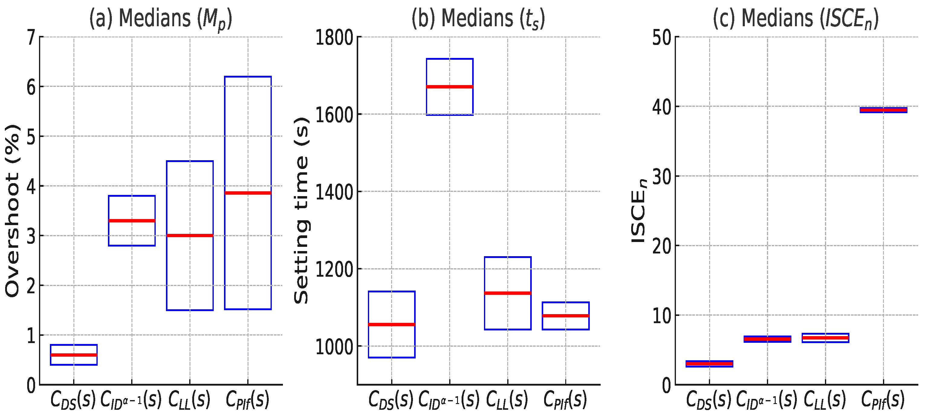
5.3. Inferential Statistical Analysis

We conducted Lilliefors and Levene tests in Matlab on the histogram data of $M_p$, $t_s$, and $ISC{E}_n$ shown in Figure 6 for each controller. The analyses revealed that none of the distributions exhibited normal behavior or homogeneous standard deviations, failing to meet the homoscedasticity conditions necessary for variance analysis. Therefore, we decided to use the Kruskal–Wallis test to determine if there were any differences in the medians of $M_p$, $t_s$, and $ISC{E}_n$ among each controller. Figure 9 shows the post-Kruskal–Wallis multiple comparison analysis. It reveals that the $C_{DS}$ controller demonstrates superior performance compared to the other controllers ($C_{I{D}^{\alpha -1}}$, $C_{LL}$, and $C_{PIDf}$) in the three examined parameters with a statistically significant distinction. With the exception of $t_s$, the medians of the parameters of the other controllers are closely grouped together, indicating that there are no significant variations in their performance in terms of overshoot and control effort. Using the post hoc test for multiple comparisons, we determined the confidence intervals for the means of each controller, detailed in

Table 4. Performance comparison of $M_p$, $t_s$, and $ISCE$ for $C_{DS}$, $C_{I{D}^{\alpha -1}}$, $C_{LL}$, and $C_{PIDf}$.

Parameter	${\mathit{C}}_{\mathbf{DS}}\left(\mathit{s}\right)$	${\mathit{C}}_{{\mathbf{ID}}^{\mathit{\alpha }-1}}\left(\mathit{s}\right)$	${\mathit{C}}_{\mathbf{LL}}\left(\mathit{s}\right)$	${\mathit{C}}_{\mathbf{PIDf}}\left(\mathit{s}\right)$
Median $M_p$	0.49	3.18	2.80	3.02
C. Interval	(0.41, 0.68)	(2.67, 3.55)	(0.79, 4.11)	(1.05, 4.74)
Median $t_s$ (s)	1043.8	1684.8	1134.5	1066.2
C. Interval (s)	(971.2, 1116.4)	(1546.9, 1761.2)	(1071.0, 1204.6)	(1014.7, 1083.7)
Median $ISCE$	3.21	4.61	6.91	39.28
C. Interval	(3.01, 3.36)	(4.39, 4.83)	(6.27, 7.41)	(39.06, 39.56)

and Figure 10. The $C_{DS}$ controller surpasses the other controllers ($C_{ID}$, $C_{LL}$, and $C_{PIDf}$) in relation to the three assessed parameters: $M_p$, $t_s$, and $ISCE$. The median value of 0.49 for $M_p$ with the $C_{DS}$ controller is considerably lower compared to the values of 3.18 for $C_{ID}$, 2.79 for $C_{LL}$, and 3.0236 for $C_{PIDf}$, indicating improvements of 84.6%, 82.4%, and 83.7%, correspondingly. When it comes to settling time $t_s$, $C_{DS}$ reaches a time of 1043.8 s. This is 38.0% less than $C_{ID}$’s time of 1684.8 s, 8.0% less than $C_{LL}$’s time of 1134.5 s, and 2.1% less than $C_{PIDf}$’s time of 1066.2 s. Regarding $ISC{E}_n$, $C_{DS}$ demonstrates a significant advantage with a value of 3.21, which is 30.2% lower than $C_{ID}$ (4.6), 53.5% lower than $C_{LL}$ (6.91), and 74.7% lower than $C_{PIDf}$ (12.7). The results demonstrate the effectiveness of the $C_{DS}$ controller in minimizing overshoot, attaining quicker settling times, and assuring adecuate control, demonstrating its superiority in terms of performance and energy savings.

6. Discussion

The results in Table 2 and Figure 7 reveal that, although the design specifications for all controllers are similar, the $C_{DS}$ controller outperforms the others in the nominal design and stands out by achieving reduced overshoot $M_p$ and shorter settling time $t_s$. In addition, although all controllers have a comparable integrated squared error $IS{E}_n$, $C_{DS}$ reduces the control effort $ISC{E}_n$, hence improving energy efficiency. The system’s capacity to effectively manage disturbances with lower values of $M_{per}$ and $t_{per}$ highlights its ability to maintain stability and optimize resources. This makes it a preferable option for energy-efficient and precision-critical applications. $C_{DS}$ achieves a disturbance rejection speed comparable to that of the $I{D}^{\alpha -1}$ controller and slower than that of the $C_{LL}\left(s\right)$ and $C_{PIDf}\left(s\right)$ controllers, but the $C_{DS}\left(s\right)$ controller accomplishes this performance with a lower magnitude of the control signal compared to the $I{D}^{\alpha -1}\left(s\right)$ and $C_{PIDf}\left(s\right)$ controllers. The same trend holds for white noise rejection.

In the Monte Carlo analysis, the superior performance of the $C_{DS}$ controller is confirmed compared to the other controllers. Regarding the overshoot $M_p$, this advantage is similar to that reported in the nominal case. For the settling time $t_s$, the superiority of the CDS controller is less evident, showing performance comparable to the $C_{LL}$ and PIDf controllers. Nevertheless, the $C_{DS}$ controller exhibits an even larger advantage than in the nominal case in terms of control signal effort and energy efficiency, as it enhances the $ISC{E}_n$ by over 90% in comparison to the $PI{D}_f$. Despite the fact that the Kruskal–Wallis analysis demonstrates a less pronounced improvement, it still achieves a substantial 74.7%.

Table 5. Comparison of controllers.

	${\mathit{C}}_{\mathit{D}\mathit{S}}\left(\mathit{s}\right)$	${\mathit{C}}_{{\mathit{I}\mathit{D}}^{\mathit{\alpha }-1}}\left(\mathit{s}\right)$	${\mathit{C}}_{\mathit{L}\mathit{L}}\left(\mathit{s}\right)$	${\mathit{C}}_{{\mathit{P}\mathit{I}\mathit{D}}_{\mathit{f}}}\left(\mathit{s}\right)$
Method	Analytical	Analytical	Analytical	Numerical
	(2 equations)	-Numerical	(4 equations	(FOMCON)
			Bode plots)
No. of parameters	4	3	3	5
Parameters	$M_p$, $t_s$, A, ${\omega }_t$	$M_p$, $t_s$, $M_g$	$M_p$, $t_s$, $e_{ss}$	$M_p$, $t_s$, A, ${\omega }_t$, $M_g$
Difficulty	Easy	Medium	Medium	Medium
Position in
the comparison
$M_p$	1st	4th	2nd	3rd
$t_s$	1st	4th	3rd	2nd
Energy efficiency	1st	2nd	3rd	4th
No. of parameters	2nd	3rd	3rd	1st
adjusted

contrasts controllers and optimization methods according to a variety of parameters. The Direct Synthesis controller ($C_{DS}$) is the most effective in terms of energy efficiency, overshoot ($M_p$), and settling time ($t_s$), rating first in all of these metrics. Although the fractional controller ($C_{I{D}^{\alpha -1}}$) rates second in energy efficiency, it exhibits a less favorable performance, ranking fourth in $M_p$ and $t_s$. The lead-lag compensator ($C_{LL}$) is ranked second in overshoot and third in both $t_s$ and energy efficiency, suggesting its intermediate performance. Conversely, the fractional proportional-integral-derivative controller ($C_{PI{D}_f}$) is more challenging to modify due to its increased number of parameters. It is ranked third in $M_p$ and second in $t_s$, but fourth in energy efficiency, rendering it the least efficient in terms of control effort.

7. Conclusions

Using four specifications and two equations to solve, a simple and analytical approach to developing FOCs through Direct Synthesis has been described. When compared to other controllers like fractional-order PID and ID, or integer-order lead-lag phase compensators, this technique has distinct advantages in terms of settling time, overshoot, and control signal effort. As a result, it is a desirable choice for applications where energy efficiency is crucial. Although Direct Synthesis controllers have not been as well received in the literature as fractional-order PID controllers, their primary benefit is the possibility of developing analytical design expressions, making controller parameter adjustment simpler. Although it might be assumed that system robustness would be compromised by avoiding computational optimization methods, our results from Monte Carlo analysis and other statistical tests suggest otherwise.

With the proposed method, Direct Synthesis control offers a viable alternative for controlling systems with disturbances and uncertain parameters, resulting in reduced control effort and, consequently, greater energy efficiency. This work was not approached from the perspective of robust control, where robustness is understood as the ability to meet desired operational specifications even in the presence of external disturbances and parametric uncertainties, ensuring both stable performance and reliable behavior. However, as a future research direction, it would be interesting to compare and/or complement the proposed method with robust control techniques such as QFT, $H_{\infty }$, loop shaping, and adaptive control. Future lines of work also include the exploration of strategies for the hardware implementation of controllers designed through Direct Synthesis, such as those reported in [49], the development of an analytical expression for selecting the parameter $\alpha$, and the derivation of analytical expressions for closed-loop responses different from that described in (13). Finally, to the best of the authors’ knowledge, no formal analysis has been undertaken to show that fractional systems are more robust to disturbances than integer-order systems. Nonetheless, the examination presented in Section 3.3 could be a useful place to start, especially when it comes to Direct Synthesis design.

References

1. Oustaloup, A.; Melchior, P. The great principles of the Crone control. In Proceedings of the IEEE Systems Man and Cybernetics Conference—SMC, Le Touquet, France, 17–20 October 1993; Volume 2, pp. 118–129. [Google Scholar] [CrossRef]
2. Podlubny, I. Fractional-Order Systems and Fractional-Order Controllers; Institute of Experimental Physics, Slovak Academy of Sciences: Kosice, Slovakia, 1994; Volume 12, pp. 1–18. Available online: https://igor.podlubny.website.tuke.sk/pspdf/uef0394.pdf (accessed on 1 November 2024).
3. Pérez, R.R.; García, F.C.; Moriano, J.S.; Batlle, V.F. Control robusto de orden fraccionario de la presión del vapor en el domo superior de una caldera bagacera. Rev. Iberoam. Autom. Inform. Ind. 2014, 11, 20–31. [Google Scholar] [CrossRef]
4. Memlikai, E.; Kapoulea, S.; Psychalinos, C.; Baranowski, J.; Bauer, W.; Tutaj, A.; Piatek, P. Design of fractional-order lead compensator for a car suspension system based on curve-fitting approximation. Fractal Fract. 2021, 5, 46. [Google Scholar] [CrossRef]
5. Chen, Y.Q.; Moore, K.L.; Vinagre, B.M.; Podlubny, I. Robust PID controller autotuning with an isodamping property through a phase shaper. In Fractional Differentiation and Its Applications; Ubooks Verlag: Mossautal, Germany, 2005; pp. 687–706. [Google Scholar]
6. Monje, C.A.; Vinagre, B.M.; Feliu, V.; Chen, Y. Tuning and auto-tuning of fractional order controllers for industry applications. Control. Eng. Pract. 2008, 16, 798–812. [Google Scholar] [CrossRef]
7. Fergani, N. Direct synthesis-based fractional-order PID controller design: Application to AVR system. Int. J. Dyn. Control 2022, 10, 2124–2138. [Google Scholar] [CrossRef]
8. Muresan, C.I.; Keyser, R.D. Revisiting Ziegler–Nichols: A fractional order approach. ISA Trans. 2022, 129, 287–296. [Google Scholar] [CrossRef] [PubMed]
9. Saleem, O.; Ali, S.; Iqbal, J. Robust MPPT control of stand-alone photovoltaic systems via adaptive self-adjusting fractional-order PID controller. Energies 2023, 16, 5039. [Google Scholar] [CrossRef]
10. Ghamari, S.M.; Jouybari, T.Y.; Mollaee, H.; Khavari, F.; Hajihosseini, M. Design of a novel robust adaptive cascade controller for DC-DC buck-boost converter optimized with neural network and fractional-order PID strategies. J. Eng. 2023, 2023, 12244. [Google Scholar] [CrossRef]
11. Trivedi, R.; Verma, B.; Padhy, P. Indirect optimal tuning rules for fractional-order proportional integral derivative controller. Int. J. Numer. Model. Electron. Netw. 2020, 34, e2838. [Google Scholar] [CrossRef]
12. Nassef, A.M.; Abdelkareem, M.A.; Maghrabie, H.M.; Baroutaji, A. Metaheuristic-based algorithms for optimizing fractional-order controllers—A recent, systematic, and comprehensive review. Fractal Fract. 2023, 7, 553. [Google Scholar] [CrossRef]
13. Monje, C.A.; Chen, Y.Q.; Vinagre, B.M.; Xue, D.; Feliu, V. Fractional-Order Systems and Controls: Fundamentals and Applications; Advances in Industrial Control; Springer: London, UK, 2010. [Google Scholar]
14. Chen, Y.; Petras, I.; Xue, D. Fractional order control - a tutorial. In Proceedings of the 2009 American Control Conference, St. Louis, MO, USA, 10–12 June 2009; pp. 1397–1411. [Google Scholar] [CrossRef]
15. Das, S.; Saha, S.; Das, S.; Gupta, A. On the selection of tuning methodology of FOPID controllers for the control of higher order processes. ISA Trans. 2011, 50, 376–388. [Google Scholar] [CrossRef]
16. Shah, P.; Agashe, S. Review of fractional PID controller. Mechatronics 2016, 38, 29–41. [Google Scholar] [CrossRef]
17. Muñiz-Montero, C.; García-Jiménez, L.V.; Sánchez-Gaspariano, L.A.; Sánchez-López, C.; González-Díaz, V.R.; Tlelo-Cuautle, E. New alternatives for analog implementation of fractional-order integrators, differentiators and PID controllers based on integer-order integrators. Nonlinear Dyn. 2017, 90, 241–256. [Google Scholar] [CrossRef]
18. Nie, Z.; Zheng, Y.; Wang, Q.G.; Liu, R.; Xiang, L.J. Fractional-order PID controller design for time-delay systems based on modified Bode’s ideal transfer function. IEEE Access 2020, 8, 103500–103510. [Google Scholar] [CrossRef]
19. Soukkou, A.; Belhour, M.C.; Leulmi, S. Review, design, optimization and stability analysis of fractional-order PID controller. Int. J. Intell. Syst. Appl. 2016, 8, 73. [Google Scholar] [CrossRef]
20. Laifa, S.; Boudjehem, B.; Gasmi, H. Direct synthesis approach to design fractional PID controller for SISO and MIMO systems based on Smith predictor structure applied for time-delay non-integer-order models. Int. J. Dyn. Control 2022, 10, 760–770. [Google Scholar] [CrossRef]
21. Kumar, A.; Pan, S. Design of fractional-order PID controller for load frequency control system with communication delay. ISA Trans. 2022, 129, 138–149. [Google Scholar] [CrossRef]
22. Ahmed, S. Fractional-order controller design using the direct synthesis method. In Proceedings of the 2022 IEEE International Symposium on Advanced Control of Industrial Processes (AdCONIP), Vancouver, BC, Canada, 7–9 August 2022; pp. 337–342. [Google Scholar] [CrossRef]
23. Arya, P.P.; Chakrabarty, S. A robust internal model-based fractional-order controller for fractional-order plus time delay processes. IEEE Control Syst. Lett. 2020, 4, 862–867. [Google Scholar] [CrossRef]
24. Yumuk, E.; Güzelkaya, M.; Eksin, I. Optimal fractional-order controller design using direct synthesis method. IET Control Theory Appl. 2020, 14, 2960–2967. [Google Scholar] [CrossRef]
25. Vavilala, S.K.; Thirumavalavan, V. Analytical design of the fractional order controller and robustness verification. IAES Int. J. Robot. Autom. (IJRA) 2021, 10, 10–23. [Google Scholar] [CrossRef]
26. Icmez, Y.; Can, M.S. Smith predictor controller design using the direct synthesis method for unstable second-order and time-delay systems. Processes 2023, 11, 941. [Google Scholar] [CrossRef]
27. Ajmeri, M.; Ali, A. Analytical design of modified Smith predictor for unstable second-order processes with time delay. Int. J. Syst. Sci. 2017, 48, 1671–1681. [Google Scholar] [CrossRef]
28. Nise, N.S. Control Systems Engineering, 6th ed.; Wiley: Hoboken, NJ, USA, 2011. [Google Scholar]
29. Thammarat, C.; Puangdownreong, D. CS-based optimal PIλDμ controller design for induction motor speed control system. Int. J. Electr. Eng. Inform. 2019, 11, 638–661. [Google Scholar] [CrossRef]
30. Colin-Cervantes, J.D.; Sanchez-Lopez, C.; Ochoa-Montiel, R.; Torres-Muñoz, D.; Hernandez-Mejia, C.M.; Sanchez-Gaspariano, L.A.; Gonzalez-Hernandez, H.G. Rational approximations of arbitrary order: A survey. Fractal Fract. 2021, 5, 267. [Google Scholar] [CrossRef]
31. Reddy, A.S.; Reddy, G.N. Novel applications of Oustaloup recursive approximation and modified Oustaloup recursive approximation methods in linear fractional order control design. Int. J. Dyn. Control 2024, 12, 2236–2246. [Google Scholar] [CrossRef]
32. Yuan, I.; Xiu, G.; Shi, B. Equivalence of the Initialized Riemann-Liouville Derivatives and the Initialized Caputo Derivatives. arXiv 2018, arXiv:1811.11537. [Google Scholar]
33. Merrikh-Bayat, F.; Karimi-Ghartemani, M. Some properties of three-term fractional order system. Fract. Calc. Appl. Anal. (FCAA) 2008, 11, 3. Available online: http://www.diogenes.bg/fcaa/volume11/fcaa113/FMBayat_MK%20Ghartemani_fcaa113.pdf (accessed on 1 November 2024).
34. Wang, F.Y. The exact and unique solution for phase-lead and phase-lag compensation. IEEE Trans. Educ. 2003, 46, 258–262. [Google Scholar] [CrossRef]
35. Muñiz-Montero, C.; Sánchez-Gaspariano, L.A.; Sánchez-López, C.; González-Díaz, V.R.; Tlelo-Cuautle, E. On the electronic realizations of fractional-order phase-lead-lag compensators with opamps and FPAAs. In Fractional Order Control and Synchronization of Chaotic Systems; Azar, A., Vaidyanathan, S., Ouannas, A., Eds.; Studies in Computational Intelligence; Springer: Cham, Switzerland, 2017; Volume 688, pp. 95–118. [Google Scholar] [CrossRef]
36. Kumarasamy, V.; Thottam, K.; Ramasamy, V.; Chrasekaran, G.; Chinnaraj, G.; Sivalingam, P.; Kumar, N.S. A review of integer order PID and fractional order PID controllers using optimization techniques for speed control of brushless DC motor drive. Int. J. Syst. Assur. Eng. Manag. 2023, 14, 1139–1150. [Google Scholar] [CrossRef]
37. Da Silva, C.S.; Da Silva, N.J.; Júnior, F.A.; Medeiros, R.L.; Silva, L.E.; Lucena, V.F. Experimental implementation of hydraulic turbine dynamics and a fractional order speed governor controller on a small-scale power system. IEEE Access 2024, 12, 40480–40495. [Google Scholar] [CrossRef]
38. Rahimian, M.A.; Tavazoei, M.S. Improving integral square error performance with implementable fractional-order PI controllers. Optim. Control. Appl. Methods 2014, 35, 303–323. [Google Scholar] [CrossRef]
39. Roongmuanpha, N.; Satansup, J.; Pukkalanun, T.; Tangsrirat, W. Design of mixed-mode analog PID controller with CFOAs. Sensors 2024, 24, 3125. [Google Scholar] [CrossRef]
40. Adhikari, A.; Schaffer, J. Modified Lilliefors test. J. Mod. Appl. Stat. Methods 2015, 14, 53–69. [Google Scholar] [CrossRef]
41. Schultz, B.B. Levene’s test for relative variation. Syst. Biol. 1985, 34, 449–456. [Google Scholar] [CrossRef]
42. Kruskal, W.H.; Wallis, W.A. Use of ranks in one-criterion variance analysis. J. Am. Stat. Assoc. 1952, 47, 583–621. [Google Scholar] [CrossRef]
43. Angel, L.; Viola, J. Design and statistical robustness analysis of FOPID, IOPID and SIMC PID controllers applied to a motor-generator system. IEEE Lat. Am. Trans. 2015, 13, 3724–3734. [Google Scholar] [CrossRef]
44. Makhbouche, A.; Boudjehem, B.; Birs, I.; Muresan, C.I. Fractional-order PID controller based on immune feedback mechanism for time-delay systems. Fractal Fract. 2023, 7, 53. [Google Scholar] [CrossRef]
45. Skogestad, S. Simple analytic rules for model reduction and PID controller tuning. J. Process. Control 2003, 13, 291–309. [Google Scholar] [CrossRef]
46. Li, Y.; Ang, K.H.; Chong, G.C.Y. PID control system analysis and design. IEEE Control Syst. Mag. 2006, 26, 32–41. [Google Scholar] [CrossRef]
47. Tepljakov, A.; Petlenkov, E.; Belikov, J. FOMCON: A MATLAB toolbox for fractional-order system identification and control. Int. J. Microelectron. Comput. Sci. 2011, 2, 51–62. [Google Scholar]
48. Duddeti, B.B.; Naskar, A.K.; Meena, V.; Bahadur, J.; Meena, P.K.; Hameed, I.A. FOMCON toolbox-based direct approximation of fractional order systems using gaze cues learning-based grey wolf optimizer. Fractal Fract. 2024, 8, 477. [Google Scholar] [CrossRef]
49. Muñiz-Montero, C.; Munoz-Pacheco, J.M.; Arizaga-Silva, J.A.; Martínez, W.O. Exploring Four Direct Synthesis Scenarios for Fractional-Order Controllers. Authorea 2024. [Google Scholar] [CrossRef]
Figure 1. Block diagram of the controlled system. The input signal comprises a unit step with 10% white noise, while the disturbance is a unit step at time t = 2500 s. A Monte Carlo analysis ( N = 400 ) is performed, considering 25% standard deviations in the plant parameters. The evaluation includes the following controllers: the introduced fractional-order direct synthesis control, fractional-order integral-derivative control, phase lead-lag compensator, and fractional-order proportional-integral-derivative control.
Fractalfract 09 00101 g001
Figure 2. Transient responses to a unit step input of the system (13) with ω n = 1 rad/s. (a) Responses for 0.2 ≤ α ≤ 0.8 and −0.7 ≤ ζ ≤ −0.1. (b) Responses for 0.3 ≤ α ≤ 0.9 and 0.3 ≤ ζ ≤ 0.9.
Fractalfract 09 00101 g002
Figure 3. Transient responses to a unit step input of the system (13) for negative damping values. (a) Peak value for 0.05 α 0.9 and −0.9 ≤ ζ ≤−0.05. (b) Peak time t p for 0.05 α 0.9 and −0.9 ≤ ζ ≤ −0.05.
Fractalfract 09 00101 g003
Figure 4. Responses of the system (13) for positive damping values. (a) Peak value for 0.5 α 0.9 and 0.05 ζ 0.9 . (b) Peak time t p for 0.05 α 0.9 and 0.05 ζ 0.9 .
Fractalfract 09 00101 g004aFractalfract 09 00101 g004b
Figure 5. F ( α ) from (37) with α in the interval (0.01, 0.95). The increasing behavior suggests selecting the highest possible value of α to minimize the impact of variations on the plant parameters.
Fractalfract 09 00101 g005
Figure 6. Monte Carlo simulations, with N = 400 and 25% variations in the plant parameters, conducted for the system shown in Figure 1 with G p ( s ) defined by (38) and the controllers (42)–(45). The red graphs show the system’s response with the proposed control. The broader curves represent the averaged response. Figures (ah) show the step responses and control signals. Figures (ix) display histograms for overshoot ( M p ), settling time ( t s ), normalized integrated squared error ( I S E n ), and normalized integrated square control effort ( I S C E n ).
Fractalfract 09 00101 g006
Figure 7. Relative performance metrics of the system depicted in Figure 1 using nominal parameters.
Fractalfract 09 00101 g007
Figure 8. Relative performance metrics (mean values) of the system illustrated in Figure 1 under 25% parameter variations, obtained through a Monte Carlo analysis with N = 400 .
Fractalfract 09 00101 g008
Figure 9. Post-Kruskal–Wallis multiple comparison analysis.
Fractalfract 09 00101 g009
Figure 10. Confidence intervals for the medians of each controller: (a) Medians of M p ; (b) Medians of t s ; (c) Medians of I S C E n .
Fractalfract 09 00101 g010