Article

Hybrid Fourier Series and Weighted Residual Function Method for Caputo-Type Fractional PDEs with Variable Coefficients

by
Samad Kheybari
1,*,
Farzaneh Alizadeh
2,3,
Mohammad Taghi Darvishi
4 and
Kamyar Hosseini
2,3,5
1
Faculty of Art and Science, University of Kyrenia, TRNC, Mersin 10, Kyrenia 99320, Turkey
2
Department of Mathematics, Near East University, TRNC, Mersin 10, Nicosia 99138, Turkey
3
Research Center of Applied Mathematics, Khazar University, Baku AZ1096, Azerbaijan
4
Department of Mathematics, Faculty of Science, Razi University, Kermanshah 67149, Iran
5
Faculty of Engineering and Natural Sciences, Istanbul Okan University, Istanbul 34959, Turkey
*
Author to whom correspondence should be addressed.
Fractal Fract. 2025, 9(12), 765; https://doi.org/10.3390/fractalfract9120765
Submission received: 23 October 2025 / Revised: 14 November 2025 / Accepted: 19 November 2025 / Published: 24 November 2025
(This article belongs to the Section Numerical and Computational Methods)

Abstract

This study presents a novel computational framework for approximating solutions to time-fractional partial differential equations (TFPDEs) with variable coefficients, employing the Caputo definition of fractional derivatives. TFPDEs, distinguished by their fractional-order time derivatives, inherently capture the non-local and memory-dependent dynamics observed in a wide range of physical and engineering systems. The proposed method reformulates the TFPDE into a set of decoupled fractional-order ordinary differential equations (FODEs) via Fourier expansion strategy. This decomposition facilitates analytical tractability while preserving the essential features of the original system. The initial conditions of each resulting FODE are systematically obtained from the governing equation’s initial data. Auxiliary initial value problems are formulated for each FODE to facilitate the construction of explicit particular solutions. These solutions are then synthesized through a carefully designed linear superposition, optimized to minimize the residual error across the domain of interest. This residual minimization ensures that the composite solution closely approximates the behavior of the original TFPDE, offering both accuracy and computational efficiency. Theoretical analysis demonstrates that the method is convergent. A FLOP-based analysis confirms that the proposed method is computationally efficient. The validity and effectiveness of the proposed scheme are demonstrated through a set of benchmark problems. Empirical convergence rates are compared with those from existing numerical methods in each case. The findings confirm that the proposed approach consistently achieves superior accuracy and demonstrates robust performance under a wide range of scenarios. These findings highlight the method’s potential as a powerful and versatile tool for solving complex TFPDEs in mathematical modeling and applied sciences.

1. Introduction

Fractional calculus has gained significant traction in recent decades, emerging as a robust mathematical framework for modeling complex systems with memory and hereditary properties. Operators involving fractional-order derivatives and integrals are increasingly utilized to enhance the fidelity of simulations across diverse scientific and engineering domains. Notable applications span control theory, porous media transport, chemical and biological processes, electrochemical systems, viscoelastic materials, electromagnetic wave propagation, electric railway dynamics, telecommunication systems, and kinetic reaction modeling, and even extend to economics and financial mathematics [1,2,3,4]. Fractional operators have emerged as powerful tools for constructing models that surpass classical formulations in accuracy and descriptive capability. These operators are broadly classified into local and non-local types. As shown in [5], the conformable fractional derivative represents a specific case within the general framework of local fractional derivatives. In contrast, non-local fractional operators are particularly well-suited for mathematical modeling, as they inherently account for the system’s memory by incorporating historical data—thereby yielding more faithful and robust representations of temporal dynamics.
Non-local fractional derivatives are formulated through several distinct, non-equivalent definitions, and their geometric interpretations remain an open question. Nevertheless, these operators offer a substantial advantage over classical integer-order derivatives by enabling the development of more nuanced mathematical models that more accurately reflect complex real-world dynamics. Comprehensive discussions of these operators can be found in Refs. [1,2,3]. Among the various formulations, the Riemann–Liouville and Caputo derivatives have received particular attention due to their broad applicability in modeling systems with memory and hereditary effects. The Riemann–Liouville and Caputo fractional derivatives are closely related; under suitable regularity conditions on the underlying function, one can be transformed into the other [1,2,3]. In problems involving the Riemann–Liouville derivative, the initial conditions typically require specifying fractional-order derivatives at t = 0, which may lack direct physical interpretation. In contrast, the Caputo derivative permits initial conditions to be specified using classical integer-order derivatives evaluated at t = 0 , thereby enhancing compatibility with traditional formulations of initial value problems [3,6].
This study investigates a generalized class of time-fractional partial differential equations (TFPDEs) capable of modeling a wide range of phenomena, including—but not limited to—sub-diffusive processes, modified anomalous diffusion, wave–diffusion interactions, and fractional-order telegraph-type systems [7,8,9,10,11,12,13,14,15,16,17,18,19,20,21,22,23,24,25].
D t λ 0 C v ( x , t ) + j = 1 n 1 f j ( t ) D t λ j 0 C v ( x , t ) + j = n 1 + 1 n 2 f j ( t ) D t λ j 0 C 2 v ( x , t ) x 2 + s ( x , t ) = 0 , ( x , t ) [ 0 , 1 ] × [ 0 , T ] .
In this formulation, D t λ 0 C represents the Caputo-type fractional derivative of order λ , taken with respect to time. The primary derivative order is defined by λ ( 0 , 2 ] , while each subsidiary order λ j ( 0 , λ ) , for j = 1 , , n 2 , represents an additional time-fractional component embedded within the model. The functions g j ( x , t ) and s ( x , t ) are assumed to be sufficiently smooth and specified a priori. To ensure the well-posedness of the problem, the governing Equation (1) is supplemented with appropriately defined initial conditions and boundary constraints, as outlined below.
v ( x , 0 ) = g 0 ( x ) , x [ 0 , 1 ] , for λ ( 0 , 2 ] v ( x , 0 ) t = g 1 ( x ) , x [ 0 , 1 ] , for λ ( 1 , 2 ] , v ( 0 , t ) = h 0 ( t ) , v ( 1 , t ) = h 1 ( t ) , t [ 0 , T ] .
The general formulation presented in (1) demonstrates considerable flexibility, enabling the derivation of numerous specific cases as special instances. Below are several notable examples that illustrate its breadth and applicability:
  • Time-fractional sub-diffusion models, as explored in [7,8,9,10,11], constitute a prominent subclass of fractional PDEs that describe anomalous transport phenomena in which the mean squared displacement grows sub-linearly with time. These models typically involve Caputo derivatives of order λ ( 0 , 1 ) , which capture memory effects and non-local temporal behavior. They are particularly effective in modeling processes such as contaminant diffusion in porous media, charge transport in disordered systems, and biological diffusion involving trapping mechanisms.
    D t λ 0 C v ( x , t ) κ 2 v ( x , t ) x 2 + s ( x , t ) = 0 , λ ( 0 , 1 ) , κ R + .
  • Time-fractional telegraph equations, as discussed in [12,13], extend classical telegraph models by incorporating fractional-order time derivatives, typically of the Caputo type. These equations are particularly effective in capturing the wave–diffusion duality in media exhibiting memory effects, such as viscoelastic materials or biological tissues. The fractional order λ ( 1 , 2 ] enables the modeling of damped wave propagation with non-local temporal behavior, providing a more accurate representation of signal transmission, relaxation phenomena, and anomalous transport processes.
    D t λ 0 C v ( x , t ) + κ 1 D t λ 1 0 C v ( x , t ) + κ 2 v ( x , t ) 2 v ( x , t ) x 2 + s ( x , t ) = 0 , λ ( 1 , 2 ] .
  • Multi-term time-fractional diffusion and diffusion-wave models, as introduced in [14,15,16,17], extend classical formulations by incorporating multiple fractional derivatives of distinct orders. These models are particularly effective in capturing complex memory effects and layered temporal dynamics, which are often observed in heterogeneous media and viscoelastic systems. By accommodating a combination of sub-diffusive and wave-like behaviors, multi-term formulations provide enhanced flexibility for simulating anomalous transport, relaxation phenomena, and hybrid diffusion–wave processes.
    D t λ 0 C v ( x , t ) + j = 1 n κ j D t λ j 0 C v ( x , t ) κ n + 1 2 v ( x , t ) x 2 + s ( x , t ) = 0 , 0 < λ j < λ < 2 , κ j R + .
  • Anomalous sub-diffusion equations involving fractional-time operators, as presented in [18,19,20,21,22,23,24,25], are formulated to model transport processes in which particle motion deviates from classical Brownian behavior. These equations typically involve Caputo derivatives of order λ ( 0 , 1 ) , effectively capturing long-range temporal correlations and memory effects. Such models are especially relevant in heterogeneous or disordered media, where trapping, crowding, or structural complexity gives rise to sub-linear scaling of the mean squared displacement. Owing to their flexibility and accuracy, these models serve as valuable tools in fields from geophysics and biology to materials science and finance.
    v ( x , t ) x κ 1 D t λ 1 0 C 2 v ( x , t ) x 2 + κ 2 D t λ 2 0 C 2 v ( x , t ) x 2 + s ( x , t ) = 0 , 0 < λ 1 , λ 2 < 1 , κ 1 , κ 2 R + .
Extensive investigations into the aforementioned subclasses, as documented in [26,27,28,29,30], have yielded rigorous proofs establishing well-posedness with respect to both existence and uniqueness of solutions. A substantial body of research has also focused on solving fractional-order partial differential equations (FPDEs) using the Lie symmetry method. This approach facilitates the reduction of complex FPDEs to simpler forms—either fractional PDEs or fractional ordinary differential equations (FODEs)—thereby providing a powerful analytical framework. However, despite its strengths, a persistent challenge lies in solving the resulting reduced equations, which are often analytically intractable. For readers interested in a deeper exploration of this technique and its applications, further insights can be found in [31,32].
This study aims to achieve a dual objective: first, to employ a reduction strategy for simplifying fractional partial differential equations (FPDEs); and second, to introduce a semi-analytical approach capable of producing accurate approximate solutions to the resulting reduced forms. Given the inherent complexity and analytical intractability of most FPDEs encountered in real-world applications, substantial research efforts have been devoted to developing robust computational techniques for their approximation. A comprehensive overview of the numerical methods proposed for solving FPDEs is presented below.
Numerous computational schemes have proven effective for approximating solutions to fractional partial differential equations (FPDEs). Lin et al. [7] introduced a high-accuracy numerical method where temporal integration was performed using finite difference techniques, while spatial discretization was achieved via a Legendre-based spectral collocation approach. This scheme was specifically designed for time-fractional diffusion equations. Building on this foundation, Cui [8] proposed a high-order method tailored to fractional diffusion models, combining a compact finite difference formulation for spatial derivatives with the Grünwald–Letnikov approximation for the temporal fractional operator. Khader [9] developed a hybrid computational strategy that integrates the Chebyshev collocation method with finite difference procedures, enhancing both accuracy and efficiency. In a related study, Kurt Bahşi et al. [11] developed a numerical framework for solving one-dimensional spatial fractional diffusion equations based on Fibonacci polynomials. These polynomials were transformed from their standard algebraic form into matrix-based representations, enabling efficient computation and improved stability. Several advanced computational techniques have been introduced to approximate solutions of fractional partial differential equations (FPDEs), especially in complex time–space domains. Mollahasani et al. [12] solved the time-fractional telegraph equations using an operator-based approach with hybrid Legendre–block pulse expansions. Zheng et al. [16] developed a high-order space–time spectral method for multi-term time-fractional diffusion systems, demonstrating enhanced accuracy and efficiency compared with traditional finite difference schemes.
In a complementary study, Dehghan et al. [21] developed a discretization framework combining temporal finite differences with a Legendre spectral element approach for spatial approximation, tailored to time-fractional modified anomalous sub-diffusion equations. Cao et al. [22] proposed a stable and convergent numerical scheme based on the implicit midpoint method and Grünwald–Letnikov discretization to solve non-linear variants of anomalous sub-diffusion equations. Abbaszadeh et al. [23] extended these ideas to multi-dimensional domains, by introducing a spectral element-based computational strategy for generalized sub-diffusion models. Reutskiy et al. [33] developed a numerical scheme that integrates time discretization with a collocation approach, while Reutskiy [34] further advanced this framework by constructing semi-analytical collocation schemes for multi-term FPDEs with time-dependent coefficients. Bayrak et al. [35] introduced the residual power series technique—a semi-analytical method—for deriving approximate closed-form solutions to space–time-fractional differential models. Their approach involves transforming the original equations into either spatial or temporal fractional forms, which is followed by expansion into fractional power series. In [36], a robust computational method was proposed for time–space FPDEs with variable coefficients, utilizing shifted Chebyshev polynomials and operational matrices to convert the original equation into a system of fractional ordinary differential equations (FODEs), from which optimal approximations were derived. Building on this, Kheybari et al. [37] extended a methodology to address variable-order time–space FPDEs, offering semi-analytical solutions with enhanced flexibility and accuracy.
Recent advances have introduced a variety of alternative computational frameworks proposed for addressing fractional partial differential equations (FPDEs) that incorporate both temporal and spatial components. These methods, as demonstrated in [17,25,38,39], provide enhanced flexibility and accuracy in handling complex fractional models. They employ a range of strategies—including spectral collocation, operational matrix techniques, and semi-analytical formulations—each specifically designed to address the complexities introduced by variable coefficients, multi-term fractional operators, and high-dimensional domains.
This study introduces a refined semi-analytical technique for approximating a solution to the time-fractional partial differential equation (TFPDE) defined in (1). The proposed method assumes that the solution can be expressed as a Fourier series expansion in the spatial variable, with time-dependent coefficients. Substituting this representation into the governing Equation (1) yields a system of decoupled time-fractional ordinary differential equations (FODEs), each subject to its own initial condition.
The core of the algorithm lies in solving this system of independent FODEs, since their solutions govern the temporal evolution of the Fourier coefficients. This framework builds upon the semi-analytical methods developed by Kheybari et al. [40,41], originally designed for solving λ -order ordinary differential equations with λ R + . In this work, we extend those techniques to accommodate fractional-order dynamics under prescribed initial conditions.
To compute the time-dependent coefficients, auxiliary differential equations are constructed and solved explicitly. An optimal linear combination of these particular solutions is then selected to ensure that the residual error vanishes in an average sense over the spatial domain. This guarantees that the resulting approximate solution satisfies the boundary conditions specified in (2).
The structure of this paper is as follows: Section 1 outlines the governing time-fractional partial differential Equation (1) and provides a concise review of existing numerical techniques employed in the solution of FPDEs. In Section 2, we present foundational definitions and properties of fractional operators, which establish the theoretical framework for the subsequent analysis. Section 3 details the proposed algorithm for solving TFPDEs, which is structured into four sub-sections. In the first sub-section, a Fourier expansion of the spatial variable is employed to transform the original problem into a system of decoupled time-fractional ordinary differential equations (FODEs). The second sub-section introduces an enhanced semi-analytical method for approximating the solutions of these FODEs. The third sub-section presents the convergence analysis. The fourth sub-section outlines the complete implementation procedure of the proposed scheme. Section 4 demonstrates the effectiveness of the method through a series of benchmark test problems, highlighting its accuracy and computational efficiency. Finally, Section 5 concludes the paper by summarizing and providing a critical analysis of the results.

2. Basic Definitions and Notations

This section introduces foundational concepts of fractional operators, which underpin the analytical framework developed in the subsequent sections. For a more in-depth exploration of the broader properties and theoretical developments in fractional calculus, the reader is referred to [1,3].
Definition 1 
([3]). Let f : R + R be a given function. The fractional integral of order r 0 of f is given by
J 0 r f ( x ) = 1 Γ ( r ) 0 x ( x s ) r 1 f ( s ) d s , r > 0 , x 0 , f ( x ) , r = 0 .
Since the integrand on the right-hand side is pointwise well-defined over the interval ( 0 , + ) , it is measurable and thus suitable for integration within the prescribed domain.
Definition 2 
([3]). Let f : R + R be a sufficiently smooth function. The following expression characterizes the Caputo fractional derivative of order r > 0 for the function f:
D x r 0 C f ( x ) = J 0 m r d m f ( x ) d x m = 1 Γ ( m r ) 0 x ( x s ) m r 1 d m f ( s ) d s m d s , m N , m 1 < r m , x 0 .
Remark 1. 
According to Definition 2, it follows directly that the Caputo fractional derivative of a constant function vanishes, i.e., D t λ 0 C c = 0 ,   for any constant c and λ ( 0 , 1 ) .   This property aids in formulating initial conditions by aligning with classical interpretations and simplifying homogeneous terms. Also,
D x r 0 C x α = Γ ( α + 1 ) Γ ( α r + 1 ) x α r , ( α N 0 α r ) ( α N α > [ r ] ) , 0 , α N 0 α [ r ] ,
where N 0 = N { 0 } .

3. Solution Framework and Implementation

In this section, we present a complete solution strategy to approximate the time-fractional partial differential equation (TFPDE) introduced earlier. The framework integrates analytical decomposition alongside semi-analytical approximations to effectively handle the temporal and spatial intricacies of fractional models. The method begins by expressing the solution as a Fourier series expansion in the spatial variable, thereby transforming the original TFPDE into a system of decoupled time-fractional ordinary differential equations (FODEs). These FODEs are then solved using an enhanced semi-analytical approach, which constructs exact solutions to auxiliary equations and selects an optimal linear combination that minimizes the residual error across the domain. The implementation procedure is detailed in three sub-sections, covering the transformation, approximation, and algorithmic execution of the proposed method. This section consists of four distinct parts. Each part contributes to the development and implementation of the proposed solution framework. First, the Fourier expansion technique is applied to convert the original time-fractional partial differential Equation (1) to a system of decoupled time-fractional ordinary differential equations (FODEs), each governed by its corresponding initial condition(s).
After that, a robust semi-analytical method is introduced for solving the resulting FODEs. This approach involves the construction of auxiliary equations and corresponding residual functions, which are systematically minimized using the collocation method to ensure accuracy and consistency. Next, an analytical discussion is presented, which shows that our method is convergent. Finally, a detailed algorithm is presented to implement the proposed solution strategy. This algorithm integrates the transformation, approximation, and optimization steps into a coherent computational procedure, enabling efficient and accurate approximation of the solution to the original problem.

3.1. Decomposition of the Main Equation

This section decomposes the governing Equation (1) into decoupled initial value problems of time-dependent fractional ordinary differential equations (FODEs). To facilitate this process, the boundary conditions are first transformed to homogeneous form, which simplifies the analytical treatment of the time-fractional partial differential equation (TFPDE). In order to do this, the following transformation is employed:
v ( x , t ) = ( 1 x ) h 0 ( t ) + x h 1 ( t ) + u ( x , t ) ,
where h 0 ( t ) and h 1 ( t ) are prescribed boundary functions, and u(x,t) is the unknown function satisfying homogeneous boundary conditions. Substituting the transformation (3) into the original Equation (1), and applying the linearity of the fractional derivative and spatial operators, we obtain a modified equation for u ( x , t ) that satisfies j = 1 m D t λ j 0 C u ( x , t ) + A [ u ( x , t ) ] + B [ u ( x , t ) ] + s ˜ ( x , t ) = 0 , where s ˜ ( x , t ) is the transformed source term incorporating contributions from the boundary data h 0 ( t ) and h 1 ( t ) . This formulation enables the decomposition of the problem into a series of time-fractional ordinary differential equations by expanding u ( x , t ) in terms of orthogonal spatial basis functions, as detailed in the next subsection.
D t λ 0 C u ( x , t ) + j = 1 n 1 f j ( t ) D t λ j 0 C u ( x , t ) + j = n 1 + 1 n 2 f j ( t ) D t λ j 0 C 2 u ( x , t ) x 2 + s ( x , t ) = 0 , u ( x , 0 ) g 0 ( x ) g 0 ( x ) x h 1 ( 0 ) + ( x 1 ) h 0 ( 0 ) , ( 0 x 1 ) ( 0 < λ 2 ) , u ( x , 0 ) t g 1 ( x ) g 1 ( x ) x d h 1 ( t ) d t | t = 0 + ( x 1 ) d h 0 ( t ) d t | t = 0 , ( 0 x 1 ) ( 1 < λ 2 ) , u ( 0 , t ) = u ( 1 , t ) 0 , t [ 0 , T ] ,
where the function s ( x , t ) is given by
s ( x , t ) = s ( x , t ) + ( 1 x ) D t λ 0 C h 0 ( t ) + x D t λ 0 C h 1 ( t ) + j = 1 n 1 f j ( t ) x D t λ j 0 C h 1 ( t ) + ( 1 x ) D t λ j 0 C h 0 ( t ) .
Furthermore, the Dirichlet boundary conditions are assumed to be satisfied by s ( x , t ) , g 0 ( x ) , and g 1 ( x ) . The solution of problem (4) is sought in terms of the following Fourier expansion:
u ( x , t ) = a 0 ( t ) 2 + n = 1 a n ( t ) cos 2 n π x + b n ( t ) sin 2 n π x .
For the purposes of this analysis, we assume that s ( x , t ) is represented as
s ( x , t ) = A 0 ( t ) 2 + n = 1 A n ( t ) cos ( 2 n π x ) + B n ( t ) sin ( 2 n π x ) ,
where
A 0 ( t ) = 2 0 1 s ( x , t ) d x , A n ( t ) = 2 0 1 s ( x , t ) cos ( 2 n π x ) d x , n = 1 , 2 , , B n ( t ) = 2 0 1 s ( x , t ) sin ( 2 n π x ) d x , n = 1 , 2 , .
The incorporation of (5) and (6) into (4) yields the following expression:
D t λ 0 C a 0 ( t ) 2 + n = 1 + a n ( t ) cos ( 2 n π x ) + b n ( t ) sin ( 2 n π x ) + j = 1 n 1 f j ( t ) D t λ j 0 C a 0 ( t ) 2 + n = 1 + a n ( t ) cos ( 2 n π x ) + b n ( t ) sin ( 2 n π x ) 4 π 2 j = n 1 + 1 n 2 f j ( t ) D t λ j 0 C n = 1 + n 2 a n ( t ) cos ( 2 n π x ) + b n ( t ) sin ( 2 n π x ) + A 0 ( t ) 2 + n = 1 A n ( t ) cos ( 2 n π x ) + B n ( t ) sin ( 2 n π x ) = 0 .
Accordingly, the equation can be reformulated as follows:
1 2 D t λ 0 C a 0 ( t ) + j = 1 n 1 f j ( t ) D t λ j 0 C a 0 ( t ) + A 0 ( t ) + n = 1 + D t λ 0 C a n ( t ) + j = 1 n 1 f j ( t ) D t λ j 0 C a n ( t ) 4 π 2 n 2 j = n 1 + 1 n 2 f j ( t ) D t λ j 0 C a n ( t ) + A n ( t ) cos ( 2 n π x ) + n = 1 + D t λ 0 C b n ( t ) + j = 1 n 1 f j ( t ) D t λ j 0 C b n ( t ) 4 π 2 n 2 j = n 1 + 1 n 2 f j ( t ) D t λ j 0 C b n ( t ) + B n ( t ) sin ( 2 n π x ) = 0 .
Let us denote the following assumption:
g 0 ( x ) = u ( x , 0 ) = a 0 ( t ) 2 + n = 1 + a n ( 0 ) cos ( 2 n π x ) + b n ( 0 ) sin ( 2 n π x ) , where a 0 ( 0 ) = 2 0 1 g 0 ( x ) d x = a 0 , 0 , a n ( 0 ) = 2 0 1 g 0 ( x ) cos ( 2 n π x ) d x = a n , 0 , n = 1 , 2 , , b n ( 0 ) = 2 0 1 g 0 ( x ) sin ( 2 n π x ) d x = b n , 0 , n = 1 , 2 , .
In the case where λ ( 1 , 2 ] , we assume that
g 1 ( x ) = u ( x , 0 ) t = d a 0 ( t ) d t 2 + n = 1 + d a n ( 0 ) d t cos ( 2 n π x ) + d b n ( 0 ) d t sin ( 2 n π x ) , where d a 0 ( 0 ) d t = 2 0 1 g 1 ( x ) d x = a ˙ 0 , 0 , d a n ( 0 ) d t = 2 0 1 g 1 ( x ) cos ( 2 n π x ) d x = a ˙ n , 0 , n = 1 , 2 , , d b n ( 0 ) d t = 2 0 1 g 1 ( x ) sin ( 2 n π x ) d x = b ˙ n , 0 , n = 1 , 2 , .
Utilizing (7), (8), and (9), the system reduces to the following fully decoupled initial value problem:
D t λ 0 C a 0 ( t ) + j = 1 n 1 f j ( t ) D t λ j 0 C a 0 ( t ) + A 0 ( t ) = 0 , a 0 ( 0 ) = a 0 , 0 , if   λ ( 0 , 2 ] , d a 0 ( 0 ) d t = a ˙ 0 , 0 , if   λ ( 1 , 2 ] , D t λ 0 C a n ( t ) + j = 1 n 1 f j ( t ) D t λ j 0 C a n ( t ) 4 π 2 n 2 j = n 1 + 1 n 2 f j ( t ) D t λ j 0 C a n ( t ) + A n ( t ) = 0 , n = 1 , 2 , , a n ( 0 ) = a n , 0 , if   λ ( 0 , 2 ] , d a n ( 0 ) d t = a ˙ n , 0 , if   λ ( 1 , 2 ] , D t λ 0 C b n ( t ) + j = 1 n 1 f j ( t ) D t λ j 0 C b n ( t ) 4 π 2 n 2 j = n 1 + 1 n 2 f j ( t ) D t λ j 0 C b n ( t ) + B n ( t ) = 0 , n = 1 , 2 , , b n ( 0 ) = b n , 0 , if   λ ( 0 , 2 ] , d b n ( 0 ) d t = b ˙ n , 0 , if   λ ( 1 , 2 ] .

3.2. Solution of the Obtained Independent Time-Fractional ODEs (10)

The initial value problems specified by (10) are addressed by constructing an approximate solution via a validated semi-analytical technique that balances analytical tractability with computational efficiency. The approach begins by formulating a set of auxiliary initial value problems derived from (10), each possessing known exact solutions. For each mode n, the solution to (10) is then approximated as a linear combination of these auxiliary solutions, carefully chosen to satisfy the prescribed initial conditions. The coefficients c a 0 , m , c a n , m , and c b n , m appearing in the linear combinations are initially undetermined and must be computed. Their optimal values are obtained by minimizing the residual associated with the original equation, ensuring that the constructed approximation adheres closely to the dynamics governed by (10).
To determine the associated coefficients, the approximate solutions are substituted into the governing Equation (10), yielding a set of residual functions that quantify the deviation from exact satisfaction of the equation. By enforcing the condition that these residuals vanish throughout the domain—typically at a set of strategically chosen collocation points—an algebraic system is constructed. Solving this system provides explicit values for the unknown coefficients c a 0 , m , c a n , m , and c b n , m , thereby completing the approximation. A notable strength of this technique lies in its ability to generate accurate approximate solutions without relying on mesh-based discretization or any form of linearization. This mesh-free, semi-analytical framework offers both computational efficiency and analytical transparency, making it particularly well-suited for fractional-order models with complex temporal dynamics. To approximate the solution of each IVP in (10), we assume that their solutions can be represented by the following functions:
a 0 ( t ) α a 0 ( t ) + m = 0 M c a 0 , m β a 0 , m ( t ) = a ˜ 0 M ( t ) , a n ( t ) α a n ( t ) + m = 0 M c a n , m β a n , m ( t ) = a ˜ n M ( t ) , n = 1 , 2 , 3 , , b n ( t ) α b n ( t ) + m = 0 M c b n , m β b n , m ( t ) = b ˜ n M ( t ) , n = 1 , 2 , 3 , ,
For n = 1 , 2 , 3 , , and m = 0 , 1 , 2 , , M , where M N denotes an arbitrary positive integer, the coefficients c a 0 , m , c a n , m , and c b n , m are initially undetermined and will be computed subsequently. Furthermore, the functions α a 0 ( t ) , β a 0 , m ( t ) , α a n ( t ) , β a n , m ( t ) , α b n ( t ) , and β b n , m ( t ) are chosen suitably to ensure that a ˜ 0 M ( t ) , a ˜ n M ( t ) , and b ˜ n M ( t ) satisfy the initial conditions prescribed in (10), namely
for 0 < λ 2 : a ˜ 0 M ( 0 ) = α a 0 ( 0 ) + m = 0 M c a 0 , m β a 0 , m ( 0 ) = a 0 , 0 , a ˜ n M ( 0 ) = α a n ( 0 ) + m = 0 M c a n , m β a n , m ( 0 ) = a n , 0 , n = 1 , 2 , 3 , , b ˜ n M ( 0 ) = α b n ( 0 ) + m = 0 M c b n , m β b n , m ( 0 ) = b n , 0 , n = 1 , 2 , 3 , , for 1 < λ 2 : d a ˜ 0 M ( 0 ) d t = d α a 0 ( 0 ) d t + m = 0 M c a 0 , m d β a 0 , m ( 0 ) d t = a ˙ 0 , 0 , d a ˜ n M ( 0 ) d t = d α a n ( 0 ) d t + m = 0 M c a n , m d β a n , m ( 0 ) d t = a ˙ n , 0 , n = 1 , 2 , 3 , , d b ˜ n M ( 0 ) d t = d α b n ( 0 ) d t + m = 0 M c b n , m d β b n , m ( 0 ) d t = b ˙ n , 0 , n = 1 , 2 , 3 , .
The functions a ˜ 0 M ( t ) , a ˜ n M ( t ) , and b ˜ n M ( t ) are consistent with the initial condition (10), provided the subsequent conditions are met:
for 0 < λ 2 : α a 0 ( 0 ) = a 0 , 0 , β a 0 , m ( 0 ) = 0 , α a n ( 0 ) = a n , 0 , β a n , m ( 0 ) = 0 , α b n ( 0 ) = b n , 0 , β b n , m ( 0 ) = 0 , for 1 < λ 2 : d α a 0 ( 0 ) d t = a ˙ 0 , 0 , d β a 0 , m ( 0 ) d t = 0 , d α a n ( 0 ) d t = a ˙ n , 0 , d β a n , m ( 0 ) d t = 0 , d α b n ( 0 ) d t = b ˙ n , 0 , d β b n , m ( 0 ) d t = 0 .
Thus, the goal is to appropriately define the functions α a 0 ( t ) , β a 0 , m ( t ) , α a n ( t ) , β a n , m ( t ) , α b n ( t ) , and β b n , m ( t ) , for m = 0 , 1 , 2 , , M , and n = 1 , 2 , 3 , , so that the following independent auxiliary initial value problems are satisfied:
D t λ 0 C α a 0 ( t ) = A 0 ( t ) , α a 0 ( 0 ) = a 0 , 0 , d α a 0 ( 0 ) d t = a ˙ 0 , 0 ( if 1 < λ 2 ) , D t λ 0 C β a 0 , m ( t ) = t m · δ , β a 0 , m ( 0 ) = 0 , d β a 0 , m ( 0 ) d t = 0 ( if 1 < λ 2 ) , D t λ 0 C α a n ( t ) = A n ( t ) , α a n ( 0 ) = a n , 0 , d α a n ( 0 ) d t = a ˙ n , 0 ( if 1 < λ 2 ) , D t λ 0 C β a n , m ( t ) = t m · δ , β a n , m ( 0 ) = 0 , d β a n , m ( 0 ) d t = 0 ( if 1 < λ 2 ) , D t λ 0 C α b n ( t ) = B n ( t ) , α b n ( 0 ) = b n , 0 , d α b n ( 0 ) d t = b ˙ n , 0 ( if 1 < λ 2 ) , D t λ 0 C β b n , m ( t ) = t m · δ , β b n , m ( 0 ) = 0 , d β b n , m ( 0 ) d t = 0 ( if 1 < λ 2 ) .
The term t m · δ represents a Müntz-type polynomial defined over the interval [ 0 , 1 ] , where m = 0 , 1 , , M , and δ ( 0 , 1 ] . Notably, the accuracy of the proposed method exhibits minimal sensitivity to variations in the parameter δ . For a more detailed exposition, the reader is referred to [42,43]. By performing a fractional integration of order λ on both sides of time-fractional ordinary differential Equation (13), we obtain
α a 0 ( t ) = 0 t ( t s ) λ 1 Γ ( λ ) A 0 ( s ) d s + a 0 , 0 , 0 < λ 1 , 0 t ( t s ) λ 1 Γ ( λ ) A 0 ( s ) d s + a 0 , 0 + a ˙ 0 , 0 t , 1 < λ 2 , β a 0 ( t ) = Γ ( m · δ + 1 ) Γ ( λ + m · δ + 1 ) t m · δ + λ , 0 < λ 2 , α a n ( t ) = 0 t ( t s ) λ 1 Γ ( λ ) A n ( s ) d s + a n , 0 , 0 < λ 1 , 0 t ( t s ) λ 1 Γ ( λ ) A n ( s ) d s + a n , 0 + a ˙ n , 0 t , 1 < λ 2 , β a n ( t ) = Γ ( m · δ + 1 ) Γ ( λ + m · δ + 1 ) t m · δ + λ , 0 < λ 2 , α b n ( t ) = 0 t ( t s ) λ 1 Γ ( λ ) B n ( s ) d s + b n , 0 , 0 < λ 1 , 0 t ( t s ) λ 1 Γ ( λ ) B n ( s ) d s + b n , 0 + b ˙ n , 0 t , 1 < λ 2 , β b n ( t ) = Γ ( m · δ + 1 ) Γ ( λ + m · δ + 1 ) t m · δ + λ , 0 < λ 2 .
Furthermore, the relations (11) and (14) yield
a ˜ 0 M ( t ) = 0 t ( t s ) λ 1 Γ ( λ ) A 0 ( s ) d s + m = 0 M c a 0 , m Γ ( m · δ + 1 ) Γ ( λ + m · δ + 1 ) t m · δ + λ + a 0 , 0 , 0 < λ 1 , 0 t ( t s ) λ 1 Γ ( λ ) A 0 ( s ) d s + m = 0 M c a 0 , m Γ ( m · δ + 1 ) Γ ( λ + m · δ + 1 ) t m · δ + λ + a 0 , 0 + a ˙ 0 , 0 t , 1 < λ 2 , a ˜ n M ( t ) = 0 t ( t s ) λ 1 Γ ( λ ) A n ( s ) d s + m = 0 M c a n , m Γ ( m · δ + 1 ) Γ ( λ + m · δ + 1 ) t m · δ + λ + a n , 0 , 0 < λ 1 , 0 t ( t s ) λ 1 Γ ( λ ) A n ( s ) d s + m = 0 M c a n , m Γ ( m · δ + 1 ) Γ ( λ + m · δ + 1 ) t m · δ + λ + a n , 0 + a ˙ n , 0 t , 1 < λ 2 , b ˜ n M ( t ) = 0 t ( t s ) λ 1 Γ ( λ ) B n ( s ) d s + m = 0 M c b n , m Γ ( m · δ + 1 ) Γ ( λ + m · δ + 1 ) t m · δ + λ + b n , 0 , 0 < λ 1 , 0 t ( t s ) λ 1 Γ ( λ ) B n ( s ) d s + m = 0 M c b n , m Γ ( m · δ + 1 ) Γ ( λ + m · δ + 1 ) t m · δ + λ + b n , 0 + b ˙ n , 0 t , 1 < λ 2 .
To determine the unknown parameters c a 0 , m , c a n , m , and c b n , m , we construct the residual functions by substituting the approximated expressions a ˜ 0 M ( t ) , a ˜ n M ( t ) , and b ˜ n M ( t ) into (10), namely
R a ˜ 0 M ( t ; c a 0 ) = D t λ 0 C a ˜ 0 M ( t ) + j = 1 n 1 f j ( t ) D t λ j 0 C a ˜ 0 M ( t ) + A 0 ( t ) , R a ˜ n M ( t ; c a n ) = D t λ 0 C a ˜ n M ( t ) + j = 1 n 1 f j ( t ) D t λ j 0 C a ˜ n M ( t ) 4 π 2 n 2 j = n 1 + 1 n 2 f j ( t ) D t λ j 0 C a ˜ n M ( t ) + A n ( t ) , R b ˜ n M ( t ; c b n ) = D t λ 0 C b ˜ n M ( t ) + j = 1 n 1 f j ( t ) D t λ j 0 C b ˜ n M ( t ) 4 π 2 n 2 j = n 1 + 1 n 2 f j ( t ) D t λ j 0 C b ˜ n M ( t ) + B n ( t ) ,
where the coefficient vectors c a 0 = c a 0 , 0 , , c a 0 , M , c a n = c a n , 0 , , c a n , M , and c b n = c b n , 0 , , c b n , M are determined by minimizing the residual functions in (16) or by setting them to zero over the interval [ 0 , T ] . This is achieved by enforcing R a ˜ 0 M ( t ; c a 0 ) , R a ˜ n M ( t ; c a 0 ) , and R b ˜ n M ( t ; c a 0 ) to vanish at M + 1 collocation points given by
t k = T 2 1 + cos k π M , k = 0 , 1 , , M .
After determining the coefficient vectors c a 0 ,   c a n , and c b n , the associated functions a ˜ 0 M ( t ) , a ˜ n M ( t ) , and b ˜ n M ( t ) are reconstructed via Equation (15). These functions are subsequently employed to formulate the N-term truncated approximate solution
u ˜ N , M ( x , t ) = a ˜ 0 M ( t ) 2 + n = 1 N a ˜ n M ( t ) cos ( 2 n π x ) + b ˜ n M ( t ) sin ( 2 n π x ) .
Applying the transformation specified in (3), the approximate solution to the original Equation (1) achieves the following form:
v ˜ N , M ( x , t ) = a ˜ 0 M ( t ) 2 + n = 1 N a ˜ n M ( t ) cos ( 2 n π x ) + b ˜ n M ( t ) sin ( 2 n π x ) + x h 1 ( t ) + ( 1 x ) h 0 ( t ) .

3.3. Convergence Analysis

Applying the Caputo derivative of order λ with respect to time yields the following equations:
D t λ 0 C a ˜ 0 M ( t ) = A 0 ( t ) + m = 0 M c a 0 , m t m δ , D t λ 0 C a ˜ n M ( t ) = A n ( t ) + m = 0 M c a n , m t m δ , D t λ 0 C b ˜ n M ( t ) = B n ( t ) + m = 0 M c b n , m t m δ .
From Equations (16) and (18), the residual functions can be written as
R a ˜ 0 M ( t ; c a 0 ) = m = 0 M c a 0 , m t m δ + j = 1 n 1 f j ( t ) D t λ j 0 C a ˜ 0 M ( t ) , R a ˜ n M ( t ; c a n ) = m = 0 M c a n , m t m δ + j = 1 n 1 f j ( t ) D t λ j 0 C a ˜ n M ( t ) 4 π 2 n 2 j = n 1 + 1 n 2 f j ( t ) D t λ j 0 C a ˜ n M ( t ) , R b ˜ n M ( t ; c b n ) = m = 0 M c b n , m t m δ + j = 1 n 1 f j ( t ) D t λ j 0 C b ˜ n M ( t ) 4 π 2 n 2 j = n 1 + 1 n 2 f j ( t ) D t λ j 0 C b ˜ n M ( t ) .
The following theorem ensures that the coefficients c a 0 can be chosen such that | R a ˜ 0 M ( t ; c a 0 ) | becomes arbitrarily small:
Theorem 1. 
Assume that { f j ( t ) } j = 1 n 1 have convergent Fourier series over domain [ 0 , 1 ] . Then, for any ε > 0 , there exists an integer M 0 N such that
M M 0 , t [ 0 , 1 ] : | R a ˜ 0 M ( t ; c a 0 ) | < ε .
Proof. 
Under the above assumptions, R a ˜ 0 M ( t ; c a 0 ) has a convergent Fourier series on [ 0 , 1 ] . Therefore, it admits a Fourier series expansion of the form
R a ˜ 0 M ( t ; c a 0 ) = a ^ 0 + m = 1 a ^ m cos ( m π t ) + b ^ m sin ( m π t ) ,
where the Fourier coefficients are given by
a ^ m = 2 0 1 R a ˜ 0 M ( t ; c a 0 ) cos ( m π t ) d t , b ^ m = 2 0 1 R a ˜ 0 M ( t ; c a 0 ) sin ( m π t ) d t ,
for m = 1 , 2 , , and a ^ 0 = 0 1 R a ˜ 0 M ( t ; c a 0 ) d t . By setting
a ^ m = 0 0 m M , b ^ m = 0 , 1 m M ,
we obtain a linear system that determines the coefficients c a 0 for m = 0 , 1 , , M . Then, the residual can be expressed as the tail of the Fourier series:
R a ˜ 0 M ( t ; c a 0 ) = m = M + 1 a ^ m cos ( m π t ) + b ^ m sin ( m π t ) .
As | cos ( m π t ) | 1 , and | sin ( m π t ) | 1 , we have
| R a ˜ 0 M ( t ; c a 0 ) | m = M + 1 ( | a ^ m | + | b ^ m | ) .
Since R a ˜ 0 M is continuous, its Fourier series converges uniformly on [ 0 , 1 ] . Hence, for every ε > 0 , there exists M 0 N such that
m = M + 1 ( | a ^ m | + | b ^ m | ) < ε , M M 0 .
This completes the proof.
Remark 2. 
Following the same argument as in Theorem 1, assume that { f j ( t ) } j = 1 n 2 are continuous on [ 0 , 1 ] . Then, for any ε > 0 , there exists M 0 N such that
M M 0 , t [ 0 , 1 ] : | R a ˜ n M ( t ; c a n ) | < ε , | R b ˜ n M ( t ; c b n ) | < ε .
Remark 3. 
It should be noted that function F admits a convergent Fourier series, comprising both sine and cosine terms, provided that it satisfies the Dirichlet conditions [44]. In particular, these conditions are
  • The integral | F ( t ) | d t exists and is finite;
  • F ( t ) possesses a finite number of local extrema over its domain;
  • F ( t ) contains a finite number of finite discontinuities.
Overall, these conditions are relatively mild and are satisfied by many common functions.

3.4. Computational Procedure Corresponding to the Introduced Method

This section delineates the step-by-step procedure underlying the proposed scheme. The overall sequence of operations employed to solve Equation (1) is formally summarized in Algorithm 1, which provides an efficient and systematic implementation of the method.
Algorithm 1: Hybrid Fourier Series and Weighted Residual Function Method for Solving FPDE (1)
Input:  N , M N , δ ( 0 , 1 ] .
s ( x , t ) = s ( x , t ) + x D t λ 0 C h 1 ( t ) + ( 1 x ) D t λ 0 C h 0 ( t ) + j = 1 n 1 f j ( t ) x D t λ j 0 C h 1 ( t ) + ( 1 x ) D t λ j 0 C h 0 ( t ) ;
g 0 ( x ) g 0 ( x ) x h 1 ( 0 ) + ( x 1 ) h 0 ( 0 ) ;
if  1 < λ 2   then
    g 1 ( x ) g 1 ( x ) x d h 1 ( 0 ) d t + ( x 1 ) d h 0 ( 0 ) d t ;
end if
for   k = 0 : M   do
    t k = T 2 1 + cos k π M ;
end for
A 0 ( t ) = 2 0 1 s ( x , t ) d x ;
a 0 , 0 = 2 0 1 g 0 ( x ) d x ;
if   1 < λ 2   then
    a ˙ 0 , 0 = 2 0 1 g 1 ( x ) d x ;
end if
if   0 < λ 1   then
    a ˜ 0 M ( t ) = 0 t ( t s ) λ 1 Γ ( λ ) A 0 ( s ) d s + m = 0 M c a 0 , m Γ ( m · δ + 1 ) Γ ( λ + m · δ + 1 ) t m · δ + λ + a 0 , 0 ;
else if   1 < λ 2   then
    a ˜ 0 M ( t ) = 0 t ( t s ) λ 1 Γ ( λ ) A 0 ( s ) d s + m = 0 M c a 0 , m Γ ( m · δ + 1 ) Γ ( λ + m · δ + 1 ) t m · δ + λ + a 0 , 0 + a ˙ 0 , 0 t ;
   for  n = 1 : N  do
      a ˙ n , 0 = 2 0 1 g 1 ( x ) cos ( 2 n π x ) d x ;
      b ˙ n , 0 = 2 0 1 g 1 ( x ) sin ( 2 n π x ) d x ;
   end for
end if
R a ˜ 0 M ( t ; c a 0 ) = D t λ 0 C a ˜ 0 M ( t ) + j = 1 n 1 f j ( t ) D t λ j 0 C a ˜ 0 M ( t ) + A 0 ( t ) ;
Solve R a ˜ 0 M ( t 0 ; c a 0 ) = 0 , R a ˜ 0 M ( t 1 ; c a 0 ) = 0 , , R a ˜ 0 M ( t M ; c a 0 ) = 0 , c a 0 , 0 , c a 0 , 1 , , c a 0 , M ;
Construct:  a ˜ 0 M ( t ) ;
for   n = 1 : N   do
    A n ( t ) = 2 0 1 s ( x , t ) cos ( 2 n π x ) d x ;
    B n ( t ) = 2 0 1 s ( x , t ) sin ( 2 n π x ) d x ;
    a n , 0 = 2 0 1 g 0 ( x ) cos ( 2 n π x ) d x ;
    b n , 0 = 2 0 1 g 0 ( x ) sin ( 2 n π x ) d x ;
   if  0 < λ 1  then
      a ˜ n M ( t ) = 0 t ( t s ) λ 1 Γ ( λ ) A n ( s ) d s + m = 0 M c a n , m Γ ( m · δ + 1 ) Γ ( λ + m · δ + 1 ) t m · δ + λ + a n , 0 ;
      b ˜ n M ( t ) = 0 t ( t s ) λ 1 Γ ( λ ) B n ( s ) d s + m = 0 M c b n , m Γ ( m · δ + 1 ) Γ ( λ + m · δ + 1 ) t m · δ + λ + b n , 0 ;
else if   1 < λ 2   then
      a ˜ n M ( t ) = 0 t ( t s ) λ 1 Γ ( λ ) A n ( s ) d s + m = 0 M c a n , m Γ ( m · δ + 1 ) Γ ( λ + m · δ + 1 ) t m · δ + λ + a n , 0 + a ˙ n , 0 t ;
      b ˜ n M ( t ) = 0 t ( t s ) λ 1 Γ ( λ ) B n ( s ) d s + m = 0 M c b n , m Γ ( m · δ + 1 ) Γ ( λ + m · δ + 1 ) t m · δ + λ + b n , 0 + b ˙ n , 0 t ;
   end if
    R a ˜ n M ( t ; c a n ) = D t λ 0 C a ˜ n M ( t ) + j = 1 n 1 f j ( t ) D t λ j 0 C a ˜ n M ( t ) 4 π 2 n 2 j = n 1 + 1 n 2 f j ( t ) D t λ j 0 C a ˜ n M ( t ) + A n ( t ) ;
    Solve R a ˜ n M ( t 0 ; c a n ) = 0 , R a ˜ n M ( t 1 ; c a n ) = 0 , , R a ˜ n M ( t M ; c a n ) = 0 , c a n , 0 , c a n , 1 , , c a n , M ;
   Construct:  a ˜ n M ( t ) ;
    R b ˜ n M ( t ; c b n ) = D t λ 0 C b ˜ n M ( t ) + j = 1 n 1 f j ( t ) D t λ j 0 C b ˜ n M ( t ) 4 π 2 n 2 j = n 1 + 1 n 2 f j ( t ) D t λ j 0 C b ˜ n M ( t ) + B n ( t ) ;
    Solve R b ˜ n M ( t 0 ; c b n ) = 0 , R b ˜ n M ( t 1 ; c b n ) = 0 , , R b ˜ n M ( t M ; c b n ) = 0 , c b n , 0 , c b n , 1 , , c b n , M ;
   Construct:  b ˜ n M ( t ) ;
end for
v ˜ N , M ( x , t ) = a ˜ 0 M ( t ) 2 + n = 1 N a ˜ n M ( t ) cos ( 2 n π x ) + b ˜ n M ( t ) sin ( 2 n π x ) + x h 1 ( t ) + ( 1 x ) h 0 ( t ) .

4. Illustrative Examples

Benchmark problems are used to assess the proposed method’s performance. Each example is carefully selected to highlight different aspects of the scheme’s applicability and precision. For each case,
  • The exact solution is used as a reference;
  • The numerical solution is computed using the developed method;
  • Error metrics, including absolute error, relative error, and root mean square error (RMSE), are evaluated to quantify accuracy;
  • Computational efficiency is discussed, including convergence behavior and sensitivity to parameters such as λ , M, and N.
The results are presented in tabular and graphical formats to facilitate comparisons. These visualizations clearly demonstrate that the proposed scheme achieves the following:
  • Has high accuracy across a range of test cases.
  • Exhibits robustness with respect to variations in fractional order λ and discretization parameters.
  • Maintains stability and convergence even for stiff or singular problems.
Simulations were performed in MATLAB R2024 on a high-performance computing platform featuring an Intel Core i9-13900HX CPU and 16 GB of system memory.
The following convergence criteria are used to evaluate error dynamics and algorithm efficacy:
  • Max absolute error (M.A.E.):
    E max ( N , M ) = max 0 x 1 0 t T v ˜ N , M ( x , t ) v ( x , t ) .
  • Relative error (R.E.):
    E Rel ( N , M ) = j = 1 J k = 1 K v ˜ N , M x j , t k v x j , t k 2 j = 1 J k = 1 K v x j , t K 2 .
  • Root mean square of errors (R.M.S.E.):
    E RMS ( N , M ) = 1 J K j = 1 J k = 1 K v ˜ N , M ( x j , t k ) v ( x j , t k ) 2 .
In this section, the convergence analysis is performed using a discretized domain, where the spatial and temporal mesh resolutions are defined as J = K = 200 . The computational grid is constructed with mesh points given by
x j , t k = j J , k T K , j = 1 , 2 , , J , k = 1 , 2 , , K .
Furthermore, let E present one of the aforementioned error criteria. The observed convergence rate is then expressed as
C n , m E ( N , M ) = log E ( N , M ) E ( N + n , M + m ) .
Practically, the relation C n , m E ( N , M ) = establishes that augmenting the truncation level of the Fourier expansion in (17) from N to N + n , together with extending the components β a 0 ( t ) , β a n ( t ) , and β b n ( t ) in (12) from M + 1 to M + m + 1 , reduces the maximum error E by a factor of 10 .
Problem 1. 
The following form of the TFPDE is analyzed:
D t λ 0 C v ( x , t ) + D t λ 1 0 C v ( x , t ) 2 v ( x , t ) x 2 + s ( x , t ) = 0 , λ 1 < λ ( 1 , 2 ] , ( x , t ) [ 0 , 1 ] 2 , v ( x , 0 ) = 0 , v ( x , 0 ) t = 0 , 0 x 1 , v ( 0 , t ) = 0 , v ( 1 , t ) = 0 , 0 t 1 .
The source term is defined as
s ( x , t ) = sin ( π x ) π 2 t 3 + 6 t 3 λ 1 Γ ( 4 λ 1 ) + 6 t 3 λ Γ ( 4 λ ) ,
which has the exact solution v ( x , t ) = t 3 sin ( π x ) . The problem formulated in (20) was previously investigated by Dehghan et al. [14], where a compact finite difference scheme was employed to obtain its numerical solution. In the present study, we perform a detailed comparison between the results generated by our proposed algorithm and those reported in [14]. Table 1 summarizes this comparison across different values of λ and λ 1 , highlighting the accuracy and consistency of the developed method. The results clearly demonstrate the superior accuracy of the present method, with errors decreasing rapidly as N increases. For example, for ( λ , λ 1 ) = ( 1.9 , 1.3 ) , E max reduces from 1.126 × 10 2 at N = 10 to 4.556 × 10 16 at N = 160 . This trend is consistent across all tested cases, indicating both high convergence rates and robustness of the proposed scheme compared to the reference method. Furthermore, Table 2 reports the maximum absolute error ( E max ) , relative error ( E Rel ) , and root mean square error ( E RMS ) , along with corresponding experimental convergence rates, obtained for different parameter combinations of λ, λ 1 , and δ = 0.5 , with M = 10 and varying N. Several key observations can be drawn from Table 2. First, the proposed method demonstrates high accuracy, as the maximum absolute error decreases rapidly with increasing N, reaching extremely small values on the order of 10 16 for N = 160 , even with a relatively small number of basis functions ( M = 10 ). Second, the experimental convergence rates C 20 , 0 E max , C 20 , 0 E Rel , and C 20 , 0 E RMS remain consistent, confirming the reliability and stability of the method. Third, the errors are slightly larger for higher fractional orders (e.g., λ = 1.9 , and λ 1 = 1.3 ) at lower N, but they rapidly diminish as N increases, indicating that the method efficiently handles different fractional dynamics. Finally, although CPU time increases with N due to larger system sizes, the rapid error decay justifies the computational cost in view of the high accuracy achieved.
Overall, Table 2 confirms that the proposed method is highly accurate, rapidly convergent, and robust for a range of fractional orders.
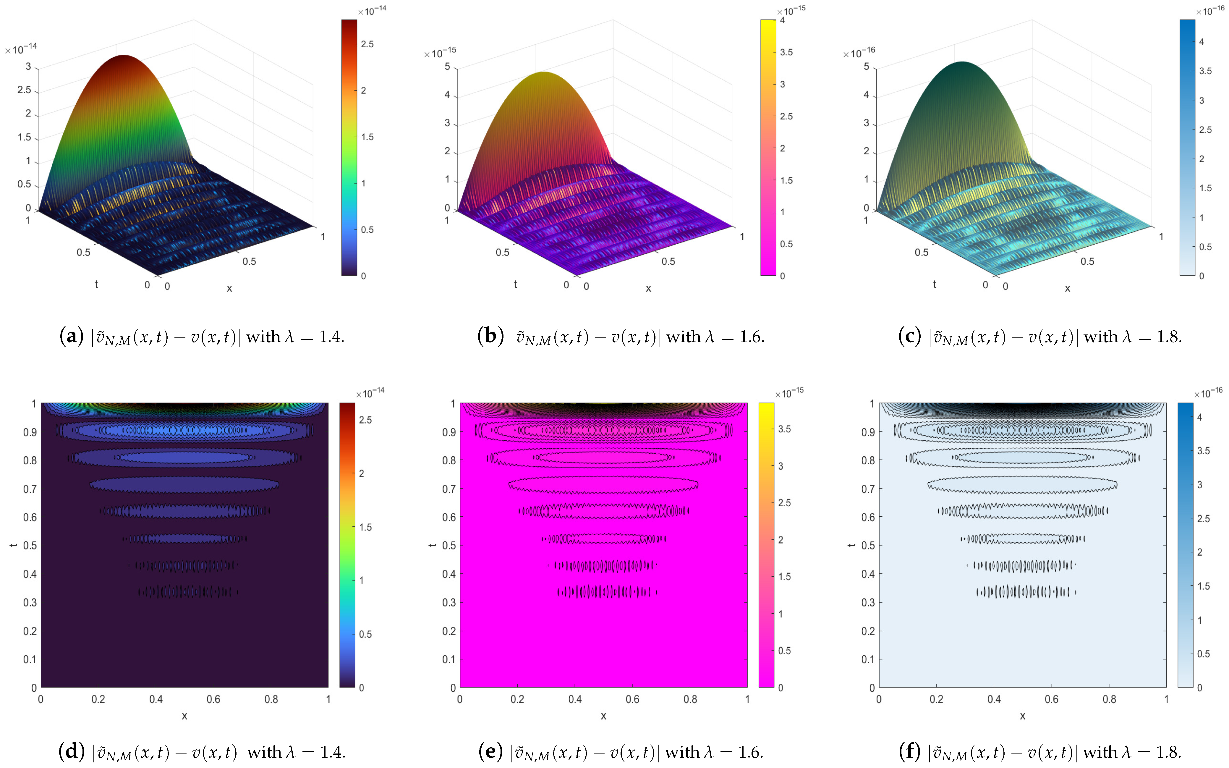
Figure 1 visualizes the absolute error function for Problem 1 using 3D surface and 2D contour plots, with parameters δ = 0.5 , M = 10 , and N = 160 , for different values of the fractional orders λ and λ 1 . The results demonstrate that the absolute error remains extremely small across the domain, reaching values on the order of 10 16 for large N, which confirms the high accuracy and rapid convergence of the proposed method. The close agreement between the numerical and exact solutions is evident from both the surface and contour plots, indicating uniformly small error indicators across all tested cases.
Problem 2. 
We examine the following time-fractional wave equation with damping:
D t λ 0 C v ( x , t ) + v ( x , t ) t 2 v ( x , t ) x 2 2 t 2 2 x ( 1 x ) t 2 λ Γ ( 3 λ ) + t = 0 , λ ( 1 , 2 ] , ( x , t ) [ 0 , 1 ] 2 , v ( x , 0 ) = 0 , v ( x , 0 ) t = 0 , 0 x 1 , v ( 0 , t ) = 0 , v ( 1 , t ) = 0 , 0 t 1 .
This problem has the exact solution v ( x , t ) = x ( 1 x ) t 2 . The problem described in (21) was examined by Bhrawy et al. [15], who employed a spectral tau scheme based on the Jacobi operational matrix to obtain numerical approximations. In the current study, we conduct a detailed comparison between the maximum absolute errors produced by our proposed algorithm and those reported in [15]. Table 3 summarizes this comparison for different values of the fractional order λ.
The results show that our approach yields much smaller errors in all cases. For example, when λ = 1.4 , and N = 100 , the present method attains an error of order 10 10 , while the corresponding value in [15] is about 10 7 . As N increases, the error decreases rapidly, confirming the spectral accuracy of the scheme. Overall, the table indicates that the proposed algorithm is highly accurate, and performs consistently well for different values of λ.
Furthermore, Table 4 reports M.A.E. ( E max ) , R.E. ( E Rel ) , and R.M.S.E. ( E RMS ) , together with their respective experimental convergence rates and CPU times, for various values of λ. These quantities are computed for different values of λ and δ = 0.2 , using M = 10 , and different values of N. For each fixed λ, all error measures decay monotonically as N increases, confirming the high-order accuracy of the proposed algorithm. The E max values decrease from about 10 4 at N = 20 to the order between 10 14 and 10 16 at N = 160 , while the empirical convergence rates of E max lie roughly between 1.1 and 1.9 , and those of E Rel between 2.1 and 3.9 . This trend indicates rapid initial convergence followed by saturation near machine precision. CPU time grows steadily with N (from about 0.7 s at N = 20 to nearly 190 s at N = 160 ), showing that computational cost is primarily governed by the spatial resolution rather than λ. Overall, the results demonstrate that the present method achieves spectral-type convergence with excellent numerical accuracy across all tested fractional orders.
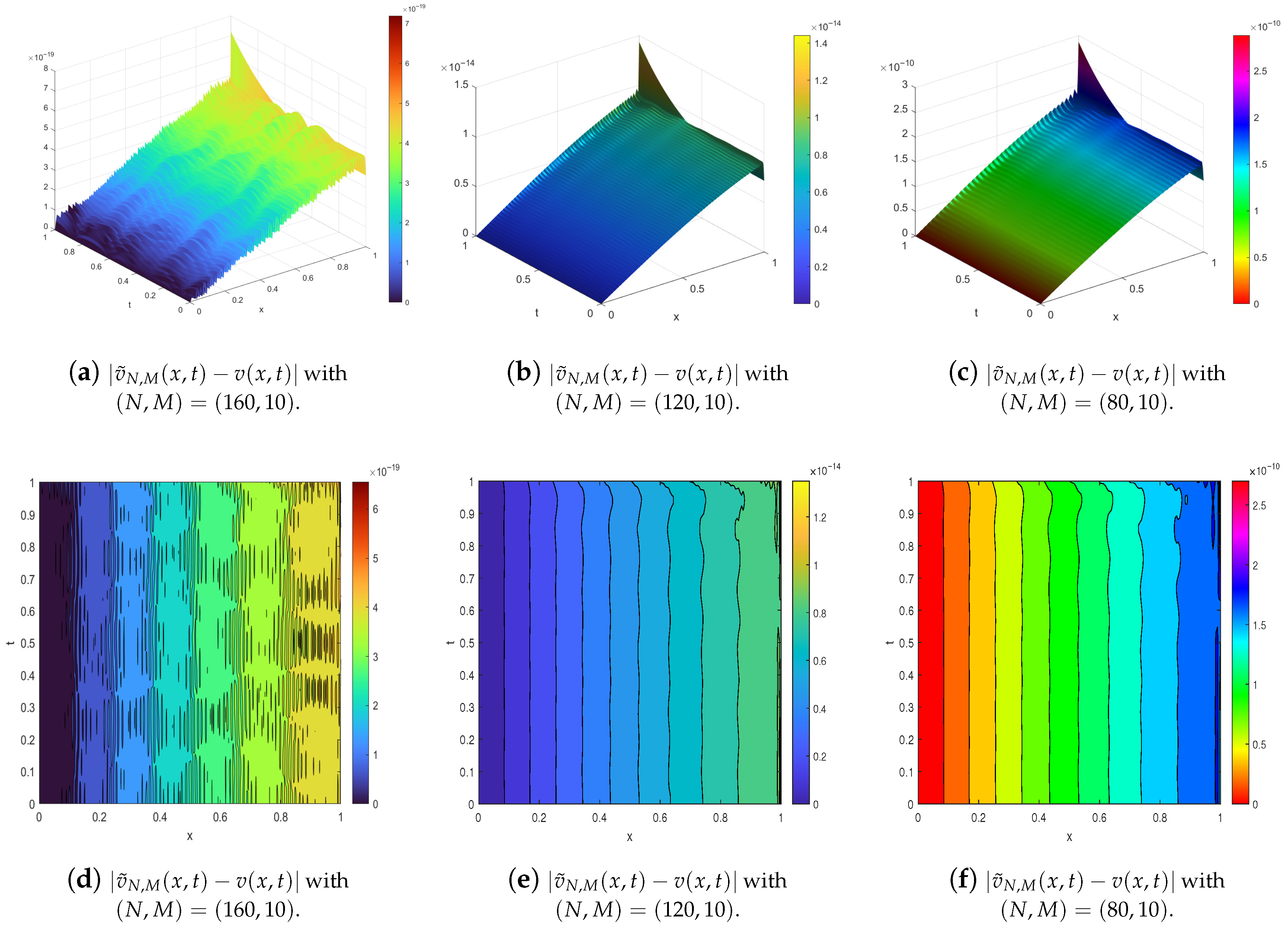
Finally, Figure 2 presents the absolute error distribution for Problem 2 using 3D surface and 2D contour plots. The results correspond to δ = 0.2 , M = 10 , and N = 160 , for various fractional orders λ. The plots show that the absolute error remains uniformly small across the entire computational domain, reaching magnitudes on the order between 10 14 and 10 16 , which clearly demonstrates the high accuracy, convergence, and robustness of the proposed numerical method.
Problem 3. 
Let us consider the following FPDE:
v ( x , t ) t D t λ 0 C 2 v ( x , t ) x 2 2 t + 8 π 2 t 2 λ Γ ( 3 λ ) sin ( 2 π x ) = 0 , λ ( 0 , 1 ] , ( x , t ) [ 0 , 1 ] 2 , v ( x , 0 ) = 0 , 0 x 1 , v ( 0 , t ) = 0 , v ( 1 , t ) = 0 , 0 t 1 .
The analytical solution for this problem can be expressed as v ( x , t ) = t 2 sin ( 2 π x ) . The problem in (22) was previously treated by Wang et al. [20], who utilized a compact finite difference scheme to compute numerical approximations. In the current study, we conduct a detailed comparison between the numerical results which are obtained by our proposed algorithm and those reported in [20]. Table 5 compares the maximum absolute errors E max at T = 1 for Problem 3 between the proposed method and the compact finite difference scheme of [20]. For all considered values of λ, our method achieves significantly smaller errors, often by several orders of magnitude, highlighting its superior accuracy and efficiency across different fractional orders and grid resolutions.
Furthermore, Table 6 reports M.A.E. ( E max ) , R.E. ( E Rel ) , and R.M.S.E. ( E RMS ) , together with their respective experimental convergence rates. These quantities are computed for different values of λ and δ = 0.2 , with different values of N and M. For each fixed fractional order λ, all error metrics decrease monotonically with increasing Fourier expansion terms N and basis functions M. The empirical convergence rates for E max range roughly from 1.3 to 2.1, and for E Rel from 2.5 to 4.5, confirming the high accuracy and effective convergence of the proposed scheme. CPU time increases with both N and M, reflecting the added computational burden of higher-resolution approximations.
Finally, Figure 3 displays the distribution of the absolute error for Problem 3, generated using 3D surface and 2D contour plots. The plots correspond to δ = 0.2 , M = 80 , and N = 80 , across different choices of the fractional order λ.
Problem 4. 
In this problem, we examine the following fractional sub-diffusion equation characterized by time-dependent coefficients:
D t λ 0 C v ( x , t ) + sin ( t ) D t λ 1 0 C v ( x , t ) sinh ( t ) D t λ 2 0 C + cosh ( t ) D t λ 3 0 C 2 v ( x , t ) x 2 + s ( x , t ) = 0 , v ( x , 0 ) = sin ( x ) , 0 x 1 , v ( 0 , t ) = 0 , v ( 1 , t ) = ( 1 + t 3 ) sin ( 1 ) , 0 t 1 .
The source term is considered as
s ( x , t ) = 6 t 3 λ Γ ( 4 λ ) + t 3 λ 1 Γ ( 4 λ 1 ) sin ( t ) + t 3 λ 2 Γ ( 4 λ 2 ) sinh ( t ) + t 3 λ 3 Γ ( 4 λ 3 ) cosh ( t ) .
The analytical solution for this problem can be expressed as v ( x , t ) = ( 1 + t 3 ) sin ( x ) . This problem was previously addressed in [36], where a shifted Chebyshev polynomial-based spectral approach was utilized to compute numerical results. This study revisits the same problem, providing a comparative analysis between our numerical approach and the results in [36]. Table 7 summarizes this comparison for λ = 0.7 , λ 1 = 0.1 , λ 2 = 0.15 , λ 3 = 0.35 , and δ = 0.3 . As observed in Table 7, the proposed method demonstrates excellent numerical accuracy and rapid convergence compared to the shifted Chebyshev spectral method reported in [36]. The maximum absolute error E max obtained by the present approach decreases exponentially as N increases, reaching values as small as 7.19 × 10 19 for N = 160 . In contrast, the reference method yields significantly larger errors for comparable discretization levels. This clear improvement highlights the superior stability and precision of the current technique, confirming its capability to efficiently capture the solution behavior even for fractional models with time-dependent coefficients.
Furthermore, Table 8 exhibits M.A.E. ( E max ) , R.E. ( E Rel ) , and R.M.S.E. ( E RMS ) , together with their respective experimental convergence rates. These quantities are computed for λ = 0.7 , λ 1 = 0.1 , λ 2 = 0.15 , λ 3 = 0.35 , and δ = 0.3 , for some values of N and M. As shown in Table 8, all error indices decrease steadily with increasing spatial collocation points N, confirming the convergence of the proposed method. The empirical convergence orders remain around 4.2 4.3 for C 20 , 0 E Rel ( N , M ) and about 2.15 for C 20 , 0 E max ( N , M ) and C 20 , 0 E RMS ( N , M ) , demonstrating spectral-like accuracy. Moreover, the CPU time exhibits only a slight increase with larger N, indicating that the method maintains high efficiency and an excellent accuracy–cost balance.
Finally, Figure 4 illustrates the absolute error function for Problem 4 using both 3D surface plots and 2D contour plots. These plots correspond to the parameters δ = 0.3 and M = 10 , and multiple values of N. As depicted in Figure 4, both the 3D surface and 2D contour plots clearly illustrate the spatial–temporal behavior of the absolute error for different values of N. It can be seen that the error magnitude decreases rapidly as N increases, demonstrating the strong convergence of the proposed scheme. Specifically, the maximum absolute error drops from the order of 10 10 for N = 80 to about 10 19 for N = 160 . The error distribution exhibits a smooth and symmetric pattern with slightly higher concentrations near the domain boundaries, which is typical for fractional diffusion-type problems. These observations confirm the numerical stability and spectral-like accuracy of the presented method.
Problem 5. 
The following time-fractional telegraph equation is investigated in this example:
D t λ 0 C v ( x , t ) + D t λ 1 0 C v ( x , t ) + v ( x , t ) 2 v ( x , t ) x 2 + s ( x , t ) = 0 , ( x , t ) [ 0 , 1 ] 2 , v ( x , 0 ) = 0 , v ( x , 0 ) t = exp ( x ) , 0 x 1 , v ( 0 , t ) = t λ + 3 + t , v ( 1 , t ) = t λ + 3 + t exp ( 1 ) , 0 t 1 .
The source term is given by
s ( x , t ) = exp ( x ) Γ ( λ + 4 ) 6 t 3 + Γ ( λ + 4 ) 24 t 4 + 1 Γ ( 3 λ ) t 2 λ .
The analytical solution for this problem can be expressed as v ( x , t ) = exp ( x ) t + t λ + 3 . This problem was previously addressed by Xu et al. [13], who applied a Legendre wavelet method to obtain numerical results. This study revisits the problem, offering a comparative analysis of our numerical approach and the results reported in [13]. Table 9 presents M.A.E. ( E max ) for various values of λ. Table 9 shows that the proposed method achieves very high accuracy for all tested values of λ. The maximum absolute error E max decreases rapidly as ( N , M ) increase, outperforming the Legendre wavelet approach in [13] by several orders of magnitude.
Furthermore, Table 10 exhibits M.A.E. ( E max ) , R.E. ( E Rel ) , and R.M.S.E. ( E RMS ) , together with their respective experimental convergence rates. These quantities are computed for δ = 0.1 and different values of λ, M and N. Table 10 demonstrates that all error measures decrease rapidly as ( N , M ) increase, confirming the high accuracy of the proposed method. The experimental convergence rates remain consistently within the ranges 1.94 2.18 for E max and E RMS , and 3.88 4.36 for E Rel , indicating a spectral-like convergence behavior. Although the CPU time grows with increasing ( N , M ) , it does so moderately, reflecting the efficiency of the algorithm even for dense discretizations. Overall, the results confirm a good balance between accuracy and computational cost.
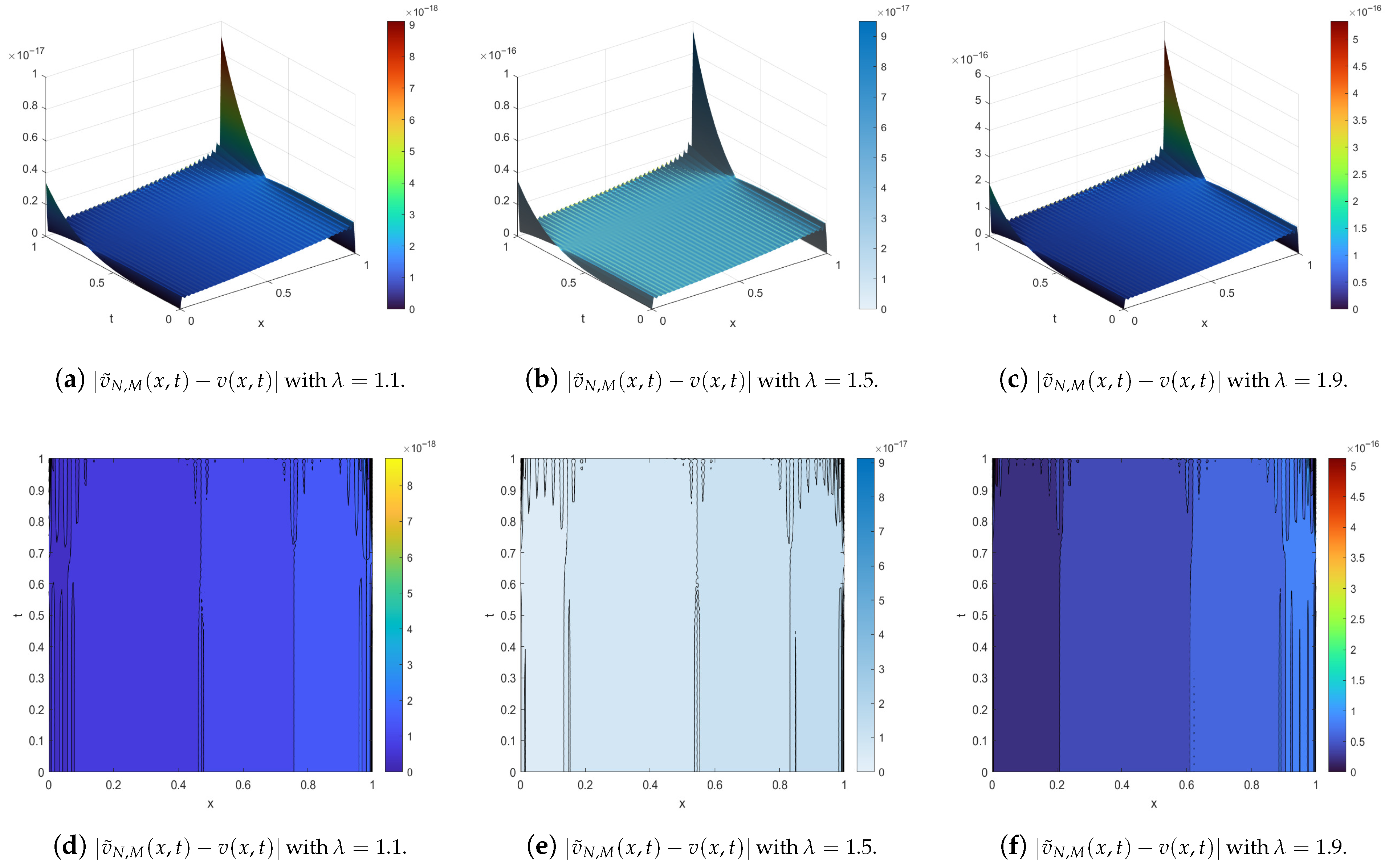
Figure 5 presents the absolute error distribution for Problem 5, using 3D surface and 2D contour plots with M = N = 80 and various values of λ ( λ = 1.1 , 1.5 , 1.9 ). As shown, the maximum absolute error increases slightly from approximately 10 18 for λ = 1.1 to 10 16 for λ = 1.9 . This increase is indicative of the growing stiffness of the problem as λ rises, which makes the numerical solution more challenging. Nevertheless, the error remains extremely small for all considered values of λ, confirming the high accuracy of the proposed numerical scheme. The results demonstrate that the method maintains robustness and reliability even for stiffer instances of the time-fractional telegraph equation.
Problem 6. 
Consider the time-fractional telegraph equations
D t λ 0 C v ( x , t ) + D t λ 1 0 C v ( x , t ) + 2 v ( x , t ) 2 v ( x , t ) x 2 + s ( x , t ) = 0 , ( x , t ) [ 0 , 1 ] 2 , v ( x , 0 ) = exp x 2 , v ( x , 0 ) t = exp x 2 , 0 x 1 , v ( 0 , t ) = exp ( t ) , v ( 1 , t ) = exp ( 1 + t ) , 0 t 1 .
The source term is considered as
s ( x , t ) = exp x 2 + t 4 x 2 1 Γ 3 2 0 x exp s 2 d s .
The closed-form solution of this problem is v ( x , t ) = exp x 2 + t . Xu et al. [13] previously addressed this equation using Legendre wavelets for numerical approximation. In the present study, we perform a comparative analysis between the absolute errors obtained by our method and those reported in [13] for Problem 6. Table 11 provides a summary of this comparison for the parameters λ = 1.5 , λ 1 = 0.5 , and δ = 0.5 . It is evident that our method achieves significantly smaller errors at all considered points ( x , t ) . In particular, for ( N , M ) = ( 80 , 80 ) , the maximum absolute error is of order O ( 10 13 ) , whereas the corresponding errors in [13] range from O ( 10 9 ) to O ( 10 11 ) . This clearly demonstrates the high accuracy and spectral-like convergence of the proposed numerical scheme. Furthermore, as ( N , M ) increase from ( 40 , 40 ) to ( 80 , 80 ) , the absolute error decreases steadily, confirming the efficiency of the method across the domain.
Furthermore, Table 12 exhibits M.A.E. ( E max ) , R.E. ( E Rel ) , and R.M.S.E. ( E RMS ) , together with their respective experimental convergence rates. These quantities are obtained for λ = 1.5 , λ 1 = 0.5 , and δ = 0.5 , with different values of N and M. The results demonstrate a rapid decrease in all error measures as ( N , M ) increase from ( 10 , 10 ) to ( 80 , 80 ) , with E max dropping from O ( 10 2 ) to O ( 10 12 ) , confirming the high accuracy of the proposed method. The experimental convergence rates are high for smaller ( N , M ) and gradually decrease for larger ( N , M ) , consistent with spectral-like convergence. CPU time increases with ( N , M ) , ranging from 0.297 s to 671.1 s, reflecting the higher computational cost of better approximation.
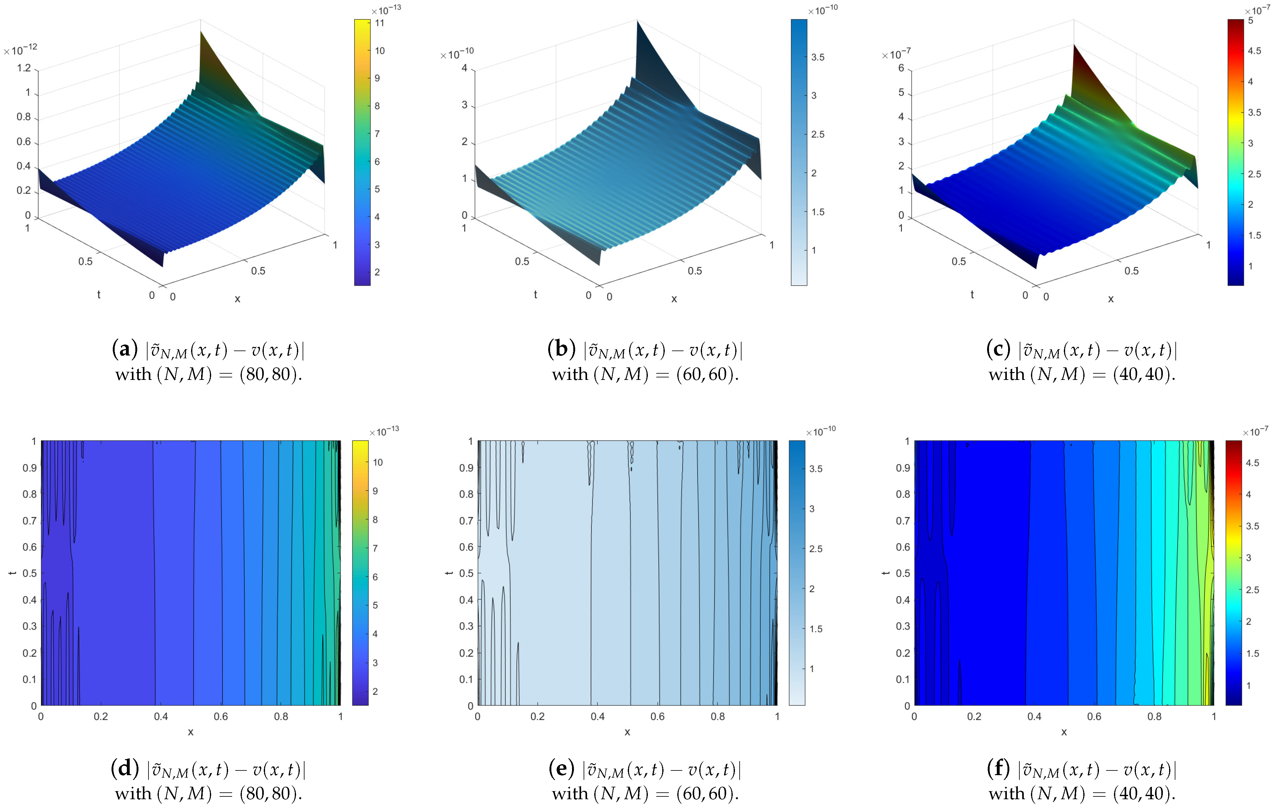
Figure 6 displays the absolute error for Problem 6. As ( M , N ) increase from ( 40 , 40 ) to ( 80 , 80 ) , the maximum absolute error decreases sharply from O ( 10 7 ) to O ( 10 13 ) , confirming the high accuracy and rapid convergence of the proposed method. The 3D surface and 2D contour plots clearly depict the error distribution across the domain.
Problem 7. 
The last benchmark is the following time-fractional telegraph equation:
D t λ 0 C v ( x , t ) + D t λ 1 0 C v ( x , t ) + v ( x , t ) 2 v ( x , t ) x 2 + s ( x , t ) = 0 , ( x , t ) [ 0 , 1 ] 2 , v ( x , 0 ) = 0 , v ( x , 0 ) t = 0 , 0 x 1 , v ( 0 , t ) = t 2 λ , v ( 1 , t ) = t 2 λ cos ( 7 ) , 0 t 1 .
Its source term is
s ( x , t ) = Γ ( 2 λ + 1 ) Γ ( λ + 1 ) t λ + Γ ( 2 λ + 1 ) Γ ( λ + 2 ) t λ + 1 + 50 t 2 λ cos ( 7 x ) .
Furthermore, its exact solution is
v ( x , t ) = t 2 λ cos ( 7 x ) .
Xu et al. [13] investigated a similar equation using a Legendre wavelet-based numerical scheme. More recently, Mulimani et al. [45] employed a powerful Taylor wavelet-based collocation technique to obtain numerical solutions for this equation. In the present study, we perform a comparative analysis between our method and those reported in [13,45]. Table 13 presents a detailed comparison of the absolute errors for Problem 7 corresponding to several values of the fractional parameter λ. Three cases, namely ( N , M ) = ( 40 , 40 ) , ( 60 , 60 ) , and ( 80 , 80 ) , were considered for our method, and the results were compared with those reported in [13,45].
As observed, the absolute errors generated by the proposed scheme are consistently smaller than those produced by existing methods across all test points and parameter values. Moreover, a clear convergence trend is observed as N and M increase in value. The error decreases rapidly as the grid is refined from ( N , M ) = ( 40 , 40 ) to ( 80 , 80 ) . Another noteworthy observation is that the errors remain very small and stable even for large values of the fractional parameter ( λ 2 ), as illustrated by the case λ = 1.99 . This indicates that the method preserves high precision and avoids numerical instability near integer-order limits, where many classical schemes lose accuracy.
Furthermore, Table 14 reports the values of M.A.E., R.E., and R.M.S.E. along with their corresponding empirical convergence rates. These errors are computed for λ = 1.25 , 1.65 , 1.95 , and 1.99 and δ = 1 , with N and M varying from 10 to 80. As shown in Table 14, all error measures decrease rapidly with increasing ( N , M ) , confirming the spectral-like accuracy of the proposed method. For example, E max drops from 6.16 × 10 3 at ( N , M ) = ( 10 , 10 ) to approximately 10 17 at ( 80 , 80 ) for λ = 1.25 . Similar exponential decay is observed for larger λ values, with convergence rates remaining nearly constant at approximately 2 for E max and E RMS , and between 3.7 and 4.4 for E Rel . For higher λ, errors rise slightly due to increased stiffness, yet the method remains precise and robust.
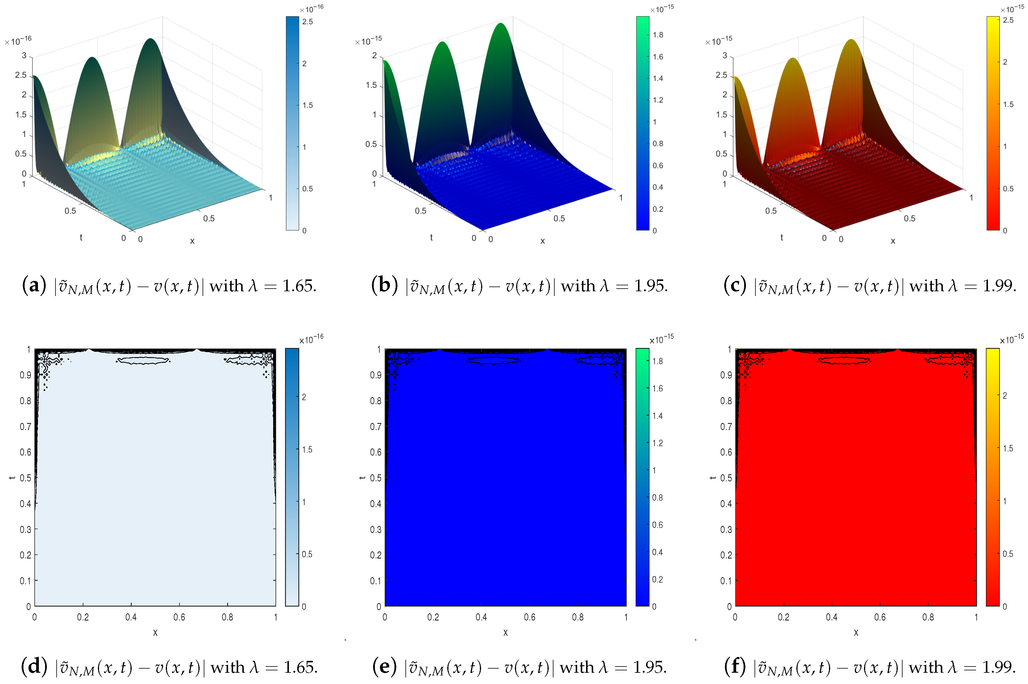
Figure 7 shows the absolute error profiles for different values of λ, with fixed parameters δ = 1 and M = N = 80 . It can be observed that as λ increases, the problem becomes slightly stiffer, leading to a minor increase in the maximum error magnitude. Nevertheless, the proposed scheme maintains very high accuracy, confirming its robustness and spectral-like convergence even under stiff parameter settings.
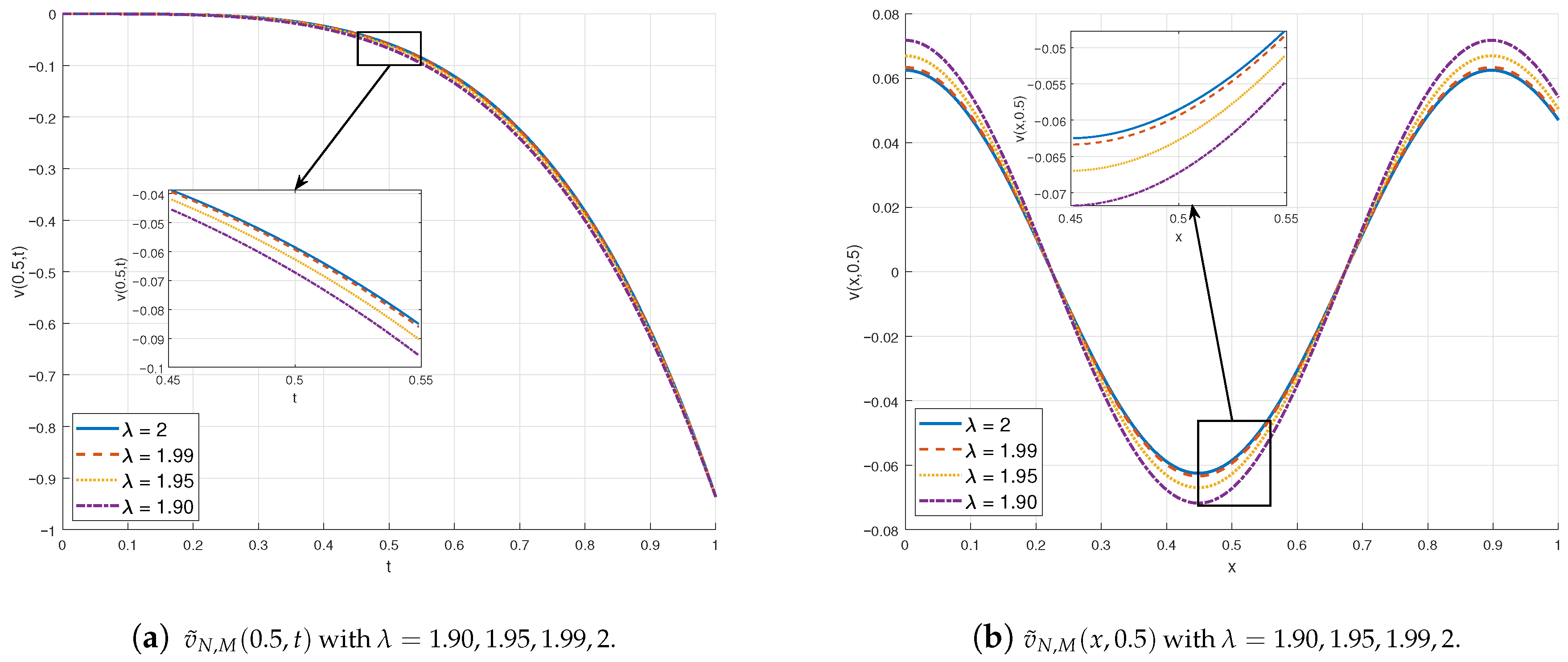
Figure 8 shows the approximate solutions of Problem 7 for different fractional orders λ. Subfigure (a) presents v ˜ N , M ( 0.5 , t ) for t [ 0 , 1 ] , while subfigure (b) shows v ˜ N , M ( x , 0.5 ) for x [ 0 , 1 ] , both corresponding to λ = 1.90 , 1.95 , 1.99 , and 2. The plots clearly demonstrate the convergence of fractional-order solutions toward the integer-order case ( λ = 2 ), thereby confirming the effectiveness of the proposed numerical method.

5. Concluding Remarks

This paper presented a robust and systematic procedure for the numerical approximation of time-fractional partial differential equations (TFPDEs) with variable coefficients, formulated in the Caputo sense. By expressing the spatial component via a Fourier series and decomposing the resulting system into independent time-fractional ordinary differential equations (FODEs), the proposed approach transforms the original problem into a more analytically and computationally tractable form. The algorithm builds upon and extends existing semi-analytical frameworks by introducing an exact resolution of auxiliary FODEs. These solutions are combined through optimally selected linear combinations that minimize the residual error in a least-squares sense, ensuring both fidelity to the governing equations and adherence to initial and boundary conditions. Convergence of the algorithm is proven analytically. Further based on a detailed FLOP count presented in Appendix A, the proposed method maintains a polynomial growth in computational cost, ensuring feasibility for real-life applications.
Based on the numerical outcomes presented in Table 1, Table 2, Table 3, Table 4, Table 5, Table 6, Table 7, Table 8, Table 9, Table 10, Table 11, Table 12, Table 13 and Table 14, a significant reduction in the error indicators—specifically E max , E Rel , and E RMS —is observed as either M or N increases. This demonstrates enhanced precision and rapid convergence of the proposed scheme. The convergence behavior, summarized in Table 2, Table 3, Table 4, Table 5, Table 6, Table 7, Table 8, Table 9, Table 10, Table 11, Table 12, Table 13 and Table 14, further confirms the stability and effectiveness of the algorithm. Notably, the comparative analysis reveals that our method surpasses the accuracy of previously established techniques. The proposed method exhibits high accuracy in solving governing Equation (1). However, as with any numerical approach, certain practical limitations exist. An increase in the parameters N (the number of Fourier terms) and M (the number of basis functions) leads to larger algebraic systems involving more unknown coefficients ( c a 0 , m , c a n , m , and c b n , m ), which consequently increases the computational cost and memory demand. In addition, the analytical forms of some integrals in (15) may not be available in general. In such cases, numerical integration techniques are required, which not only raise the computational expense but can also act as an additional source of error propagation in the overall numerical scheme. These aspects delineate the practical boundaries of the proposed method.
In summary, the proposed semi-analytical method achieves exponential convergence for a broad class of time-fractional PDEs, as verified through seven benchmark problems. The results demonstrate superior accuracy compared to existing Legendre- and wavelet-based schemes. Future work will focus on extending the approach to two-dimensional geometries and variable-coefficient models.

Author Contributions

Conceptualization, S.K. and F.A.; Methodology, S.K. and F.A.; Software, S.K. and F.A.; Formal analysis, M.T.D. and K.H.; Writing—original draft, S.K., F.A., and M.T.D.; Writing—review and editing, K.H. and M.T.D. All authors have read and agreed to the published version of the manuscript.

Funding

This research received no external funding.

Institutional Review Board Statement

Not applicable.

Informed Consent Statement

Not applicable.

Data Availability Statement

The data that support the findings of this study are available from the corresponding author upon reasonable request.

Conflicts of Interest

The authors declare no conflicts of interest.

Appendix A. Number of FLOPs

Appendix A.1. Computational Procedure Corresponding to the Proposed Method

In this section, we present the detailed computational steps that underpin the proposed numerical scheme. We analyze the computational cost of the proposed method in terms of floating-point operations (FLOPs), where each basic elementary arithmetic operation corresponds to one FLOP. This quantitative assessment measures the algorithm’s computational efficiency. Let F ( f ) denote the FLOPs required to compute a quantity f.
To estimate the computational cost of evaluating v ˜ N , M ( x , t ) , we count the FLOPs required at a given point ( x , t ) .
For each n = 1 , , N , the evaluation of
a ˜ n M ( t ) cos ( 2 n π x ) + b ˜ n M ( t ) sin ( 2 n π x ) ,
requires
F a ˜ n M ( t ) + F cos ( 2 n π x ) + F b ˜ n M ( t ) + F sin ( 2 n π x ) + 9 ,
FLOPs in total.
Hence, the overall computational cost of evaluating v ˜ N , M ( x , t ) , as defined in Equation (17), can be expressed as
F v ˜ N , M = n = 1 N F a ˜ n M ( t ) + F cos ( 2 n π x ) + F b ˜ n M ( t ) + F sin ( 2 n π x ) + F a ˜ 0 M ( t ) + F h 0 ( t ) + F h 1 ( t ) + 9 N + 4 .
The FLOPs required for a ˜ 0 M ( t ) , a ˜ n M ( t ) , and b ˜ n M ( t ) can be bounded as follows:
F a ˜ 0 M ( t ) F J 0 λ A 0 ( t ) + m = 0 M m + 9 + 5 = F J 0 λ A 0 ( t ) + M 2 + 19 M + 28 2 , F a ˜ n M ( t ) F J 0 λ A n ( t ) + m = 0 M m + 9 + 5 = F J 0 λ A n ( t ) + M 2 + 19 M + 28 2 , F b ˜ n M ( t ) F J 0 λ B 0 ( t ) + m = 0 M m + 9 + 5 = F J 0 λ B n ( t ) + M 2 + 19 M + 28 2 .
Similarly, for the fractional derivatives D t λ j 0 C a ˜ 0 M ( t ) , D t λ j 0 C a ˜ n M ( t ) , and D t λ j 0 C b ˜ n M ( t ) , where 0 λ j < λ , we have
F D t λ j 0 C a ˜ 0 M ( t ) F J 0 λ λ j A 0 ( t ) + m = 0 M m + 10 + 1 = F J 0 λ λ j A 0 ( t ) + M 2 + 21 M + 22 2 , F D t λ j 0 C a ˜ n M ( t ) F J 0 λ λ j A n ( t ) + m = 0 M m + 10 + 1 = F J 0 λ λ j A n ( t ) + M 2 + 21 M + 22 2 , F D t λ j 0 C b ˜ n M ( t ) F J 0 λ λ j B 0 ( t ) + m = 0 M m + 10 + 1 = F J 0 λ λ j B n ( t ) + M 2 + 21 M + 22 2 .

Appendix A.2. Computational Cost of Constructing the Residual Functions

The FLOPs required to construct each residual function are given by
F R a ˜ 0 M ( t ; c a 0 ) = m = 0 M [ m + 1 ] + j = 1 n 1 F f j ( t ) F D t λ j 0 C a ˜ 0 M ( t ) + 1 + 1 m = 0 M [ m + 1 ] + j = 1 n 1 F f j ( t ) F J 0 λ λ j A 0 ( t ) + M 2 + 21 M + 22 2 + 1 + 1 = M 2 + 3 M + 2 2 + j = 1 n 1 F f j ( t ) F J 0 λ λ j A 0 ( t ) + M 2 + 21 M + 22 2 + n 1 + 1 , F R a ˜ n M ( t ; c a n ) = m = 0 M [ m + 1 ] + j = 1 n 2 F f j ( t ) F D t λ j 0 C a ˜ n M ( t ) + 1 + 6 m = 0 M [ m + 1 ] + j = 1 n 2 F f j ( t ) F J 0 λ λ j A n ( t ) + M 2 + 21 M + 22 2 + 1 + 6 = M 2 + 3 M + 2 2 + j = 1 n 2 F f j ( t ) F J 0 λ λ j A n ( t ) + M 2 + 21 M + 22 2 + n 2 + 6 , F R b ˜ n M ( t ; c b n ) = m = 0 M [ m + 1 ] + j = 1 n 2 F f j ( t ) F D t λ j 0 C b ˜ n M ( t ) + 1 + 6 m = 0 M [ m + 1 ] + j = 1 n 2 F f j ( t ) F J 0 λ λ j B n ( t ) + M 2 + 21 M + 22 2 + 1 + 6 = M 2 + 3 M + 2 2 + j = 1 n 2 F f j ( t ) F J 0 λ λ j B n ( t ) + M 2 + 21 M + 22 2 + n 2 + 6 .

Appendix A.3. Formation and Solution of the Linear Systems

The construction of each system of ( M + 1 ) linear equations
{ R a ˜ 0 M ( t k ; c a 0 ) = 0 } k = 0 M , { R a ˜ n M ( t k ; c a n ) = 0 } k = 0 M , { R b ˜ n M ( t k ; c b n ) = 0 } k = 0 M ,
requires the following computational costs, respectively:
( M + 1 ) M 2 + 3 M + 2 2 + j = 1 n 1 F f j ( t ) F J 0 λ λ j A 0 ( t ) + M 2 + 21 M + 22 2 + n 1 + 1 , ( M + 1 ) M 2 + 3 M + 2 2 + j = 1 n 2 F f j ( t ) F J 0 λ λ j A n ( t ) + M 2 + 21 M + 22 2 + n 2 + 6 , ( M + 1 ) M 2 + 3 M + 2 2 + j = 1 n 2 F f j ( t ) F J 0 λ λ j B n ( t ) + M 2 + 21 M + 22 2 + n 2 + 6 .
The solution of each linear system of size ( M + 1 ) can be efficiently obtained using LU factorization. The corresponding number of floating-point operations (FLOPs) required for LU decomposition and solution are expressed as follows:
2 3 M 3 + 7 2 M 2 + 23 6 M .

Appendix A.4. Computational Cost of Constructing the Approximate Solution

The FLOPs required for constructing the residual equations and solving them to obtain c a 0 , { c a n } n = 1 N , and { c b n } n = 1 N are given by
F c = ( 2 N + 1 ) 2 3 M 3 + 7 2 M 2 + 23 6 M + ( M + 1 ) M 2 + 3 M + 2 2 + j = 1 n 1 F f j ( t ) F J 0 λ λ j A 0 ( t ) + M 2 + 21 M + 22 2 + n 1 + 1 + N ( M + 1 ) M 2 + 3 M + 2 2 + j = 1 n 2 F f j ( t ) F J 0 λ λ j A n ( t ) + M 2 + 21 M + 22 2 + n 2 + 6 + N ( M + 1 ) M 2 + 3 M + 2 2 + j = 1 n 2 F f j ( t ) F J 0 λ λ j B n ( t ) + M 2 + 21 M + 22 2 + n 2 + 6 = ( 2 N + 1 ) 7 M 3 + 33 M 2 + 38 M + 6 6 + ( M + 1 ) ( 2 N n 2 + 12 N + n 1 + 1 ) + N ( M + 1 ) j = 1 n 2 F f j ( t ) F J 0 λ λ j A n ( t ) + F J 0 λ λ j B n ( t ) + ( M 2 + 21 M + 22 ) + ( M + 1 ) j = 1 n 1 F f j ( t ) F J 0 λ λ j A 0 ( t ) + M 2 + 21 M + 22 2 .
Furthermore, the FLOPs required to construct v ˜ N , M using (A1), (A2), and the previously obtained value of F c can be expressed as
F t o t a l F c + n = 1 N [ F J 0 λ A n ( t ) + M 2 + 19 M + 28 2 + F cos ( 2 n π x ) + F J 0 λ B n ( t ) + M 2 + 19 M + 28 2 + F sin ( 2 n π x ) ] + F J 0 λ A 0 ( t ) + M 2 + 19 M + 28 2 + F h 0 ( t ) + F h 1 ( t ) + 9 N + 4 = F c + n = 1 N F J 0 λ A n ( t ) + F J 0 λ B n ( t ) + F cos ( 2 n π x ) + F sin ( 2 n π x ) + N + 1 2 M 2 + 19 M + 28 + F J 0 λ A 0 ( t ) + F h 0 ( t ) + F h 1 ( t ) + 9 N + 4 .
The total number of floating-point operations required to construct the approximate solution, F t o t a l , grows asymptotically as
F t o t a l = O ( N M 3 ) ,
where N is the number of Fourier terms, and M is the number of basis functions.
Therefore, a FLOP-based analysis shows polynomial complexity for the proposed algorithm.

References

  1. Kilbas, A.A.; Srivastava, H.M.; Trujillo, J.J. Theory and Applications of Fractional Differential Equations; North-Holland Mathematics Studies; Elsevier: Amsterdam, The Netherlands, 2006; Volume 204. [Google Scholar] [CrossRef]
  2. Das, S. Functional Fractional Calculus for System Identification and Controls; Springer: Berlin/Heidelberg, Germany, 2008. [Google Scholar] [CrossRef]
  3. Diethelm, K.; Ford, N. The Analysis of Fractional Differential Equations; Springer: Berlin/Heidelberg, Germany, 2010; Volume 2004. [Google Scholar] [CrossRef]
  4. Cui, Z.; Yu, P.; Mao, Z. Existence of solutions for nonlocal boundary value problems of nonlinear fractional differential equations. Adv. Dyn. Syst. Appl. 2012, 7, 31–40. [Google Scholar]
  5. Hashemi, M. Invariant subspaces admitted by fractional differential equations with conformable derivatives. Chaos Solitons Fractals 2018, 107, 161–169. [Google Scholar] [CrossRef]
  6. Gao, G.H.; Sun, Z.Z.; Zhang, H.W. A new fractional numerical differentiation formula to approximate the Caputo fractional derivative and its applications. J. Comput. Phys. 2014, 259, 33–50. [Google Scholar] [CrossRef]
  7. Lin, Y.; Xu, C. Finite difference/spectral approximations for the time-fractional diffusion equation. J. Comput. Phys. 2007, 225, 1533–1552. [Google Scholar] [CrossRef]
  8. Cui, M. Compact finite difference method for the fractional diffusion equation. J. Comput. Phys. 2009, 228, 7792–7804. [Google Scholar] [CrossRef]
  9. Khader, M. On the numerical solutions for the fractional diffusion equation. Commun. Nonlinear Sci. Numer. Simul. 2011, 16, 2535–2542. [Google Scholar] [CrossRef]
  10. Zeng, F.; Li, C.; Liu, F.; Turner, I. Numerical algorithms for time-fractional subdiffusion equation with second-order accuracy. SIAM J. Sci. Comput. 2015, 37, A55–A78. [Google Scholar] [CrossRef]
  11. Bahşı, A.K.; Yalçınbaş, S. Numerical solutions and error estimations for the space fractional diffusion equation with variable coefficients via Fibonacci collocation method. SpringerPlus 2016, 5, 1375. [Google Scholar] [CrossRef]
  12. Mollahasani, N.; Moghadam, M.M.M.; Afrooz, K. A new treatment based on hybrid functions to the solution of telegraph equations of fractional order. Appl. Math. Model. 2016, 40, 2804–2814. [Google Scholar] [CrossRef]
  13. Xu, X.; Xu, D. Legendre wavelets direct method for the numerical solution of time-fractional order telegraph equations. Mediterr. J. Math. 2018, 15, 1–33. [Google Scholar] [CrossRef]
  14. Dehghan, M.; Safarpoor, M.; Abbaszadeh, M. Two high-order numerical algorithms for solving the multi-term time fractional diffusion-wave equations. J. Comput. Appl. Math. 2015, 290, 174–195. [Google Scholar] [CrossRef]
  15. Bhrawy, A.; Doha, E.; Baleanu, D.; Ezz-Eldien, S. A spectral tau algorithm based on Jacobi operational matrix for numerical solution of time fractional diffusion-wave equations. J. Comput. Phys. 2015, 293, 142–156. [Google Scholar] [CrossRef]
  16. Zheng, M.; Liu, F.; Anh, V.; Turner, I. A high-order spectral method for the multi-term time-fractional diffusion equations. Appl. Math. Model. 2016, 40, 4970–4985. [Google Scholar] [CrossRef]
  17. Dehghan, M.; Abbaszadeh, M.; Deng, W. Fourth-order numerical method for the space–time tempered fractional diffusion-wave equation. Appl. Math. Lett. 2017, 73, 120–127. [Google Scholar] [CrossRef]
  18. Liu, F.; Yang, C.; Burrage, K. Numerical method and analytical technique of the modified anomalous subdiffusion equation with a nonlinear source term. J. Comput. Appl. Math. 2009, 231, 160–176. [Google Scholar] [CrossRef]
  19. Mohebbi, A.; Abbaszadeh, M.; Dehghan, M. A high-order and unconditionally stable scheme for the modified anomalous fractional sub-diffusion equation with a nonlinear source term. J. Comput. Phys. 2013, 240, 36–48. [Google Scholar] [CrossRef]
  20. Wang, Z.; Vong, S. Compact difference schemes for the modified anomalous fractional sub-diffusion equation and the fractional diffusion-wave equation. J. Comput. Phys. 2014, 277, 1–15. [Google Scholar] [CrossRef]
  21. Dehghan, M.; Abbaszadeh, M.; Mohebbi, A. Legendre spectral element method for solving time fractional modified anomalous sub-diffusion equation. Appl. Math. Model. 2016, 40, 3635–3654. [Google Scholar] [CrossRef]
  22. Cao, X.; Cao, X.; Wen, L. The implicit midpoint method for the modified anomalous sub-diffusion equation with a nonlinear source term. J. Comput. Appl. Math. 2017, 318, 199–210. [Google Scholar] [CrossRef]
  23. Abbaszadeh, M.; Dehghan, M.; Zhou, Y. Alternating direction implicit-spectral element method (ADI-SEM) for solving multi-dimensional generalized modified anomalous sub-diffusion equation. Comput. Math. Appl. 2019, 78, 1772–1792. [Google Scholar] [CrossRef]
  24. Kheybari, S.; Darvishi, M.T.; Hashemi, M.S. A semi-analytical approach to Caputo type time-fractional modified anomalous sub-diffusion equations. Appl. Numer. Math. 2020, 158, 103–122. [Google Scholar] [CrossRef]
  25. Kheybari, S.; Alizadeh, F.; Darvishi, M.T.; Hosseini, K. A Fourier Series Technique for Approximate Solutions of Modified Anomalous Time-Fractional Sub-Diffusion Equations. Fractal Fract. 2024, 8, 718. [Google Scholar] [CrossRef]
  26. Li, X.; Xu, C. Existence and uniqueness of the weak solution of the space-time fractional diffusion equation and a spectral method approximation. Commun. Comput. Phys. 2010, 8, 1016. [Google Scholar] [CrossRef]
  27. Chen, J.; Liu, F.; Anh, V. Analytical solution for the time-fractional telegraph equation by the method of separating variables. J. Math. Anal. Appl. 2008, 338, 1364–1377. [Google Scholar] [CrossRef]
  28. Jiang, H.; Liu, F.; Turner, I.; Burrage, K. Analytical solutions for the multi-term time–space Caputo–Riesz fractional advection–diffusion equations on a finite domain. J. Math. Anal. Appl. 2012, 389, 1117–1127. [Google Scholar] [CrossRef]
  29. Zaky, M.A. Existence, uniqueness and numerical analysis of solutions of tempered fractional boundary value problems. Appl. Numer. Math. 2019, 145, 429–457. [Google Scholar] [CrossRef]
  30. Stojanović, M.; Gorenflo, R. Nonlinear two-term time fractional diffusion-wave problem. Nonlinear Anal. Real World Appl. 2010, 11, 3512–3523. [Google Scholar] [CrossRef]
  31. Alizadeh, F.; Hashemi, M.S.; Haji-Badali, A. Lie symmetries, exact solutions, and conservation laws of the nonlinear time-fractional Benjamin-Ono equation. Comput. Methods Differ. Equ. 2022, 10, 608–616. [Google Scholar] [CrossRef]
  32. Alizadeh, F.; Hincal, E.; Hosseini, K.; Hashemi, M.S.; Das, A. The (2 + 1)-dimensional generalized time-fractional Zakharov Kuznetsov Benjamin Bona Mahony equation: Its classical and nonclassical symmetries, exact solutions, and conservation laws. Opt. Quantum Electron. 2023, 55, 1061. [Google Scholar] [CrossRef]
  33. Reutskiy, S.; Lin, J. A semi-analytic collocation method for space fractional parabolic PDE. Int. J. Comput. Math. 2018, 95, 1326–1339. [Google Scholar] [CrossRef]
  34. Reutskiy, S. A new semi-analytical collocation method for solving multi-term fractional partial differential equations with time variable coefficients. Appl. Math. Model. 2017, 45, 238–254. [Google Scholar] [CrossRef]
  35. Aylin Bayrak, M.; Demir, A. A new approach for space-time fractional partial differential equations by residual power series method. Appl. Math. Comput. 2018, 336, 215–230. [Google Scholar] [CrossRef]
  36. Kheybari, S. Numerical algorithm to Caputo type time–space fractional partial differential equations with variable coefficients. Math. Comput. Simul. 2021, 182, 66–85. [Google Scholar] [CrossRef]
  37. Kheybari, S.; Alizadeh, F.; Darvishi, M.T.; Hosseini, K.; Hincal, E. A Novel Semi-Analytical Scheme to Deal with Fractional Partial Differential Equations (PDEs) of Variable-Order. Fractal Fract. 2024, 8, 425. [Google Scholar] [CrossRef]
  38. Saadatmandi, A.; Dehghan, M. A new operational matrix for solving fractional-order differential equations. Comput. Math. Appl. 2010, 59, 1326–1336. [Google Scholar] [CrossRef]
  39. Dehghan, M.; Manafian, J.; Saadatmandi, A. Solving nonlinear fractional partial differential equations using the homotopy analysis method. Numer. Methods Partial. Differ. Equ. Int. J. 2010, 26, 448–479. [Google Scholar] [CrossRef]
  40. Kheybari, S.; Darvishi, M. An efficient technique to find semi-analytical solutions for higher order multi-point boundary value problems. Appl. Math. Comput. 2018, 336, 76–93. [Google Scholar] [CrossRef]
  41. Kheybari, S.; Darvishi, M.T.; Alizadeh, F.; Hincal, E.; Hosseini, K.; Chen, X. Solving Multi-Point Boundary Value Differential Equations with a Novel Semi-Analytical Algorithm. Int. J. Comput. Methods 2025, 22, 2450086. [Google Scholar] [CrossRef]
  42. Borwein, P.; Erdélyi, T.; Zhang, J. Müntz systems and orthogonal Müntz-Legendre polynomials. Trans. Am. Math. Soc. 1994, 342, 523–542. [Google Scholar] [CrossRef] [PubMed]
  43. Mokhtary, P.; Ghoreishi, F.; Srivastava, H. The Müntz-Legendre Tau method for fractional differential equations. Appl. Math. Model. 2016, 40, 671–684. [Google Scholar] [CrossRef]
  44. Jeffrey, A. Advanced Engineering Mathematics; Elsevier: Amsterdam, The Netherlands, 2001. [Google Scholar]
  45. Mulimani, M.; Kumbinarasaiah, S. Numerical solution of time-fractional telegraph equations using wavelet transform. Int. J. Dyn. Control 2024, 12, 2166–2189. [Google Scholar] [CrossRef]
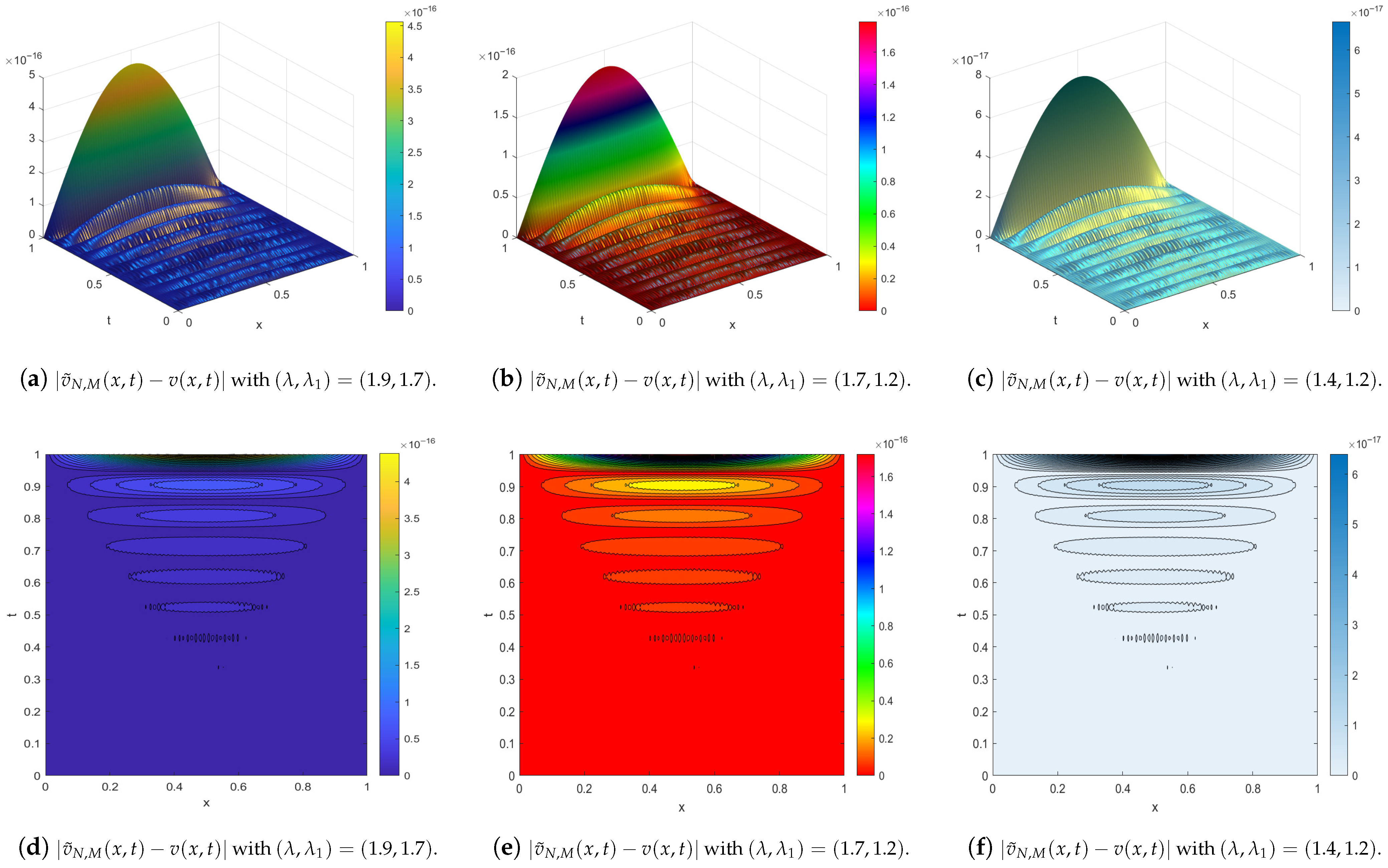
Figure 1. Visualization of the absolute error function for Problem 1 through 3D surface and 2D contour plots. The results correspond to δ = 0.5 , M = 10 , N = 160 , and various values of λ and λ 1 . It is observed that the absolute error is extremely small, reaching values on the order of 10 16 for large N, which demonstrates the high accuracy and convergence of the proposed method.
Fractalfract 09 00765 g001
Figure 2. Visualization of the absolute error for Problem 2 via 3D surface and 2D contour plots. The computations are performed with δ = 0.2 , M = 10 , and N = 160 , and for various fractional orders λ . The errors remain extremely small, on the order between 10 14 and 10 16 , confirming the high accuracy, convergence, and robustness of the proposed numerical method.
Fractalfract 09 00765 g002
Figure 3. Visualization of the absolute error for Problem 3 via 3D surface and 2D contour plots. The computations are performed with δ = 0.2 , M = 80 , and N = 80 , and for different fractional orders λ . The absolute errors remain extremely small, typically on the order of 10 15 , demonstrating the high accuracy, convergence, and robustness of the proposed numerical scheme.
Fractalfract 09 00765 g003aFractalfract 09 00765 g003b
Figure 4. Visualization of the absolute error distribution for Problem 4. Panels (ac) present 3D surface plots, while panels (df) display the corresponding 2D contour maps for δ = 0.3 , M = 10 , and various values of N ( N = 80 , 120 , 160 ). A pronounced reduction in the error amplitude is observed as N increases, with the maximum absolute error decreasing from approximately 10 10 at N = 80 to about 10 19 at N = 160 . Each plot includes a color bar that quantitatively represents the error magnitude, facilitating a clear visual comparison across different resolutions.
Fractalfract 09 00765 g004
Figure 5. Detailed graphical representation of the absolute error function for Problem 5, including 3D surface plots and 2D contour plots. The computations are performed with parameters δ = 0.1 and M = N = 80 , for various values of λ ( λ = 1.1 , 1.5 , 1.9 ). The plots show that the maximum absolute error slightly increases with λ , with values of approximately 10 18 , 10 17 , and 10 16 , respectively. This trend reflects the increasing stiffness of the problem as λ grows, while still demonstrating the high accuracy of the proposed numerical method.
Fractalfract 09 00765 g005
Figure 6. Graphical representation of the absolute error for Problem 6, including 3D surface plots and 2D contour plots. The results correspond to λ = 1.5 , λ 1 = 0.5 , and δ = 0.5 , with varying numbers of ( M , N ) . The plots illustrate that the maximum absolute error decreases significantly from approximately 10 7 to 10 13 with increasing ( M , N ) from ( 40 , 40 ) to ( 80 , 80 ) , highlighting the high accuracy and convergence of the proposed numerical method.
Fractalfract 09 00765 g006
Figure 7. Detailed graphical representation of the absolute error distribution for Problem 7, including 3D surface and 2D contour plots. The results are obtained for δ = 1 and M = N = 80 , with different values of λ ( λ = 1.65 , 1.95 , 1.99 ). The plots indicate that the maximum absolute error slightly increases with λ , reaching approximately 10 16 and 10 15 . This behavior reflects the increasing stiffness of the problem as λ grows, while the overall accuracy of the proposed numerical method remains remarkably high.
Fractalfract 09 00765 g007
Figure 8. Approximate solutions of Problem 7 obtained by the proposed method for N = M = 80 and δ = 1 . (a) shows v ˜ N , M ( 0.5 , t ) for t [ 0 , 1 ] and λ = 1.90 , 1.95 , 1.99 , and 2, while (b) presents v ˜ N , M ( x , 0.5 ) for x [ 0 , 1 ] . In both cases, the results demonstrate the convergence of the fractional-order solutions to the integer-order case λ = 2 .
Fractalfract 09 00765 g008
Table 1. Maximum absolute error comparison for Problem 1 at final time T = 1 , emphasizing the relative accuracy of the proposed scheme versus the method presented in [14].
Our ResultsMethod [14]
λ λ 1 N M E max h τ E max
1.9 1.3 1010 1.126 × 10 2 1 100 1 10 2.566 × 10 2
20 1.441 × 10 3 1 20 1.349 × 10 2
40 2.360 × 10 5 1 40 6.637 × 10 3
80 6.330 × 10 9 1 80 3.172 × 10 3
160 4.556 × 10 16 1 160 1.496 × 10 3
1.7 1.2 1010 1.032 × 10 2 1 100 1 10 6.999 × 10 3
20 1.248 × 10 3 1 20 3.855 × 10 3
40 2.360 × 10 5 1 40 1.808 × 10 3
80 6.330 × 10 9 1 80 7.925 × 10 4
160 1.787 × 10 16 1 160 3.357 × 10 4
1.4 1.2 1010 9.406 × 10 3 1 2 1 5000 1.331 × 10 2
20 1.071 × 10 3 1 4 7.822 × 10 4
40 1.391 × 10 5 1 8 4.818 × 10 5
80 2.342 × 10 9 1 16 3.141 × 10 6
160 6.644 × 10 17 1 32 3.394 × 10 7
Table 2. Error indicators—M.A.E., R.E., and R.M.S.E.—along with their corresponding convergence rates for Problem 1, using parameters δ = 0.5 , M = 10 , and N varying from 20 to 160.
λ λ 1 NMM.A.E.R.E.R.M.S.E.CPU
Time (s)
E max ( N , M ) C 20 , 0 E max ( N , M ) E Rel ( N , M ) C 20 , 0 E Rel ( N , M ) E RMS ( N , M ) C 20 , 0 E RMS ( N , M )
1.91.32010 1.44065 × 10 3 1.7857146 3.11458 × 10 7 3.5714286 1.49714 × 10 4 1.7857136 1.7031
40 2.35963 × 10 5 1.7857146 8.35547 × 10 11 3.5714283 2.45216 × 10 6 1.7857140 6.6719
60 3.86482 × 10 7 1.7857139 2.24152 × 10 14 3.5714283 4.01638 × 10 8 1.7857139 24.6094
80 6.33017 × 10 9 1.7857162 6.01332 × 10 18 3.5714288 6.57841 × 10 10 1.7857158 65.9062
100 1.03681 × 10 10 1.7857129 1.61319 × 10 21 3.5714284 1.07747 × 10 11 1.7857122 135.6406
120 1.69819 × 10 12 1.7857135 4.32770 × 10 25 3.5714174 1.76479 × 10 13 1.7857095 211.1250
140 2.78146 × 10 14 1.7857148 1.16102 × 10 28 3.5713064 2.89057 × 10 15 1.7856534 308.1406
160 4.55573 × 10 16 3.11554 × 10 32 4.73511 × 10 17 386.5312
1.71.22010 1.24750 × 10 3 1.8348610 2.33543 × 10 7 3.6697244 1.29642 × 10 4 1.8348616 1.4219
40 1.82465 × 10 5 1.8348635 4.99623 × 10 11 3.6697257 1.89620 × 10 6 1.8348622 6.6562
60 2.66880 × 10 7 1.8348618 1.06885 × 10 14 3.6697247 2.77346 × 10 8 1.8348619 24.0469
80 3.90350 × 10 9 1.8348622 2.28661 × 10 18 3.6697243 4.05658 × 10 10 1.8348623 69.3438
100 5.70942 × 10 11 1.8348623 4.89179 × 10 22 3.6697244 5.93332 × 10 12 1.8348621 107.9844
120 8.35083 × 10 13 1.8348611 1.04651 × 10 25 3.6697126 8.67832 × 10 14 1.8348577 218.4688
140 1.22143 × 10 14 1.8348631 2.23888 × 10 29 3.6696037 1.26934 × 10 15 1.8348011 299.4375
160 1.78651 × 10 16 4.79101 × 10 33 1.85685 × 10 17 391.1406
1.41.22010 1.07149 × 10 3 1.8867953 1.72289 × 10 7 3.7735856 1.11351 × 10 4 1.8867932 1.5156
40 1.39057 × 10 5 1.8867902 2.90183 × 10 11 3.7735852 1.44511 × 10 6 1.8867931 6.5625
60 1.80469 × 10 7 1.8867935 4.88750 × 10 15 3.7735846 1.87546 × 10 8 1.8867926 24.1094
80 2.34212 × 10 9 1.8867927 8.23194 × 10 19 3.7735855 2.43397 × 10 10 1.8867931 66.3906
100 3.03960 × 10 11 1.8867925 1.38649 × 10 22 3.7735852 3.15880 × 10 12 1.8867923 135.2656
120 3.94479 × 10 13 1.8867921 2.33524 × 10 26 3.7735722 4.09949 × 10 14 1.8867864 214.5156
140 5.11955 × 10 15 1.8867924 3.93332 × 10 30 3.7734639 5.32039 × 10 16 1.8867320 299.8594
160 6.64415 × 10 17 6.62667 × 10 34 6.90576 × 10 18 385.7344
Table 3. Maximum absolute error comparison for Problem 2 at final time T = 1 , emphasizing the relative accuracy of the proposed scheme versus the method presented in [15].
Our ResultsMethod [15]
λ N M E max α β τ E max
1.4 6010 1.62317 × 10 7 001 1.01 × 10 5
70 2.54038 × 10 8 11 8.67 × 10 6
80 4.16850 × 10 9 1 2 1 2 9.87 × 10 6
90 7.21905 × 10 10 1 2 1 2 7.98 × 10 6
100 1.32852 × 10 10 1 2 1 2 1.40 × 10 7
1.6 6010 5.48274 × 10 8 001 8.77 × 10 6
70 7.56330 × 10 9 11 2.01 × 10 6
80 1.10172 × 10 9 1 2 1 2 5.67 × 10 6
90 1.70734 × 10 10 1 2 1 2 9.15 × 10 6
100 2.83654 × 10 11 1 2 1 2 3.00 × 10 6
1.8 6010 1.51993 × 10 8 001 2.27 × 10 6
70 1.81492 × 10 9 11 9.75 × 10 6
80 2.30882 × 10 10 1 2 1 2 3.88 × 10 6
90 3.15583 × 10 11 1 2 1 2 7.11 × 10 6
100 4.67510 × 10 12 1 2 1 2 7.36 × 10 6
Table 4. Error indicators—M.A.E., R.E., and R.M.S.E.—along with their corresponding convergence rates for Problem 2, using parameters δ = 0.2 , M = 10 , and N varying from 20 to 160, for some values of λ .
λ NMM.A.E.R.E.R.M.S.E.CPU
Time (s)
E max ( N , M ) C 20 , 0 E max ( N , M ) E Rel ( N , M ) C 20 , 0 E Rel ( N , M ) E RMS ( N , M ) C 20 , 0 E RMS ( N , M )
1.42010 3.83382 × 10 4 1.7116929 2.53844 × 10 7 3.4233859 4.11890 × 10 5 1.7116934 0.7031
40 7.44627 × 10 6 1.6615748 9.57593 × 10 11 3.3231476 7.99996 × 10 7 1.6615737 2.9531
60 1.62317 × 10 7 1.5903842 4.55023 × 10 14 3.1807717 1.74387 × 10 8 1.5903854 7.7969
80 4.16850 × 10 9 1.4966117 3.00097 × 10 17 2.9932225 4.47846 × 10 10 1.4966104 27.3438
100 1.32852 × 10 10 1.3787880 3.04817 × 10 20 2.7575761 1.42731 × 10 11 1.3787892 61.4688
120 5.55367 × 10 12 1.2358794 5.32676 × 10 23 2.4717580 5.96663 × 10 13 1.2358792 101.1719
140 3.22627 × 10 13 1.0677240 1.79765 × 10 25 2.1344834 3.46617 × 10 14 1.0672411 143.2812
160 2.76043 × 10 14 1.31893 × 10 27 2.96899 × 10 15 190.3906
1.62010 2.26473 × 10 4 1.8370134 8.85803 × 10 8 3.6740279 2.43313 × 10 5 1.8370124 0.7344
40 3.29612 × 10 6 1.7790054 1.87633 × 10 11 3.5580105 3.54122 × 10 7 1.7790059 2.6250
60 5.48274 × 10 8 1.6969264 5.19157 × 10 15 3.3938556 5.89043 × 10 9 1.6969274 8.2812
80 1.10172 × 10 9 1.5892823 2.09625 × 10 18 3.1785595 1.18364 × 10 10 1.5892816 25.0469
100 2.83654 × 10 11 1.4547328 1.38958 × 10 21 2.9094686 3.04746 × 10 12 1.4547329 52.0625
120 9.95534 × 10 13 1.2925602 1.71165 × 10 24 2.5851194 1.06956 × 10 13 1.2925601 80.7969
140 5.07570 × 10 14 1.1031418 4.44934 × 10 27 2.2053160 5.45312 × 10 15 1.1026578 145.2812
160 4.00271 × 10 15 2.77319 × 10 29 4.30514 × 10 16 178.8594
1.82010 1.19660 × 10 4 1.9820199 2.47287 × 10 8 3.9640435 1.28558 × 10 5 1.9820235 0.7344
40 1.24718 × 10 6 1.9141056 2.68632 × 10 12 3.8282066 1.33991 × 10 7 1.9141027 2.7188
60 1.51993 × 10 8 1.8184335 3.98980 × 10 16 3.6368674 1.63295 × 10 9 1.8184337 7.9531
80 2.30882 × 10 10 1.6935992 9.20627 × 10 20 3.3872001 2.48050 × 10 11 1.6935994 23.9531
100 4.67510 × 10 12 1.5385188 3.77471 × 10 23 3.0770357 5.02273 × 10 13 1.5385188 60.1875
120 1.35292 × 10 13 1.3529414 3.16117 × 10 26 2.7058822 1.45352 × 10 14 1.3529408 106.2188
140 6.00248 × 10 15 1.1380232 6.22251 × 10 29 2.2750807 6.44882 × 10 16 1.1375404 146.0938
160 4.36825 × 10 16 3.30282 × 10 31 4.69829 × 10 17 191.5000
Table 5. Maximum absolute error comparison for Problem 3 at final time T = 1 , emphasizing the relative accuracy of the proposed scheme versus the method presented in [20].
Our ResultsMethod [20]
λ N M E max h τ E max
0.3 1010 5.36046 × 10 3 1 100 1 5 5.958 × 10 3
2020 4.11057 × 10 5 1 10 1.480 × 10 3
3030 3.60465 × 10 7 1 20 3.639 × 10 4
4040 3.87077 × 10 9 1 40 9.119 × 10 5
5050 5.46720 × 10 11 1 80 2.287 × 10 5
6060 1.09395 × 10 12 1 160 5.768 × 10 6
0.5 1010 5.72919 × 10 3 1 100 1 5 1.044 × 10 2
2020 4.86423 × 10 5 1 10 2.630 × 10 3
3030 4.69980 × 10 7 1 20 6.561 × 10 4
4040 5.51905 × 10 9 1 40 1.648 × 10 4
5050 8.43952 × 10 11 1 80 4.140 × 10 5
6060 1.80563 × 10 12 1 160 1.042 × 10 5
0.7 1010 6.10653 × 10 3 1 100 1 5 1.485 × 10 2
2020 5.71647 × 10 5 1 10 3.814 × 10 3
3030 6.06194 × 10 7 1 20 9.619 × 10 4
4040 7.75799 × 10 9 1 40 2.423 × 10 4
5050 1.28068 × 10 10 1 80 6.116 × 10 5
6060 2.92336 × 10 12 1 160 1.545 × 10 5
Table 6. Error indicators—M.A.E., R.E., and R.M.S.E.—along with their corresponding convergence rates for Problem 3, using parameters δ = 0.2 , and M and N varying from 10 to 80, for some values of λ .
λ NMM.A.E.R.E.R.M.S.E.CPU
Time (s)
E max ( N , M ) C 10 , 10 E max ( N , M ) E Rel ( N , M ) C 10 , 10 E Rel ( N , M ) E RMS ( N , M ) C 10 , 10 E RMS ( N , M )
0.31010 5.36046 × 10 3 2.1153000 3.10165 × 10 6 4.4710741 5.57621 × 10 4 2.2355355 0.4375
2020 4.11057 × 10 5 2.0570389 1.04838 × 10 10 4.2395508 3.24193 × 10 6 2.1197767 2.0625
3030 3.60465 × 10 7 1.9690657 6.03904 × 10 15 4.0165526 2.46052 × 10 8 2.0082770 7.0625
4040 3.87077 × 10 9 1.8500324 5.81320 × 10 19 3.7532467 2.41407 × 10 10 1.8766225 20.7031
5050 5.46720 × 10 11 1.6987675 1.02605 × 10 22 3.4352271 3.20721 × 10 12 1.7176133 50.8750
6060 1.09395 × 10 12 1.5147845 3.76653 × 10 26 3.0569369 6.14489 × 10 14 1.5284690 106.0781
7070 3.34359 × 10 14 1.2988546 3.30373 × 10 29 2.6178204 1.81989 × 10 15 1.3089102 274.8438
8080 1.68019 × 10 15 7.96497 × 10 32 8.93583 × 10 17 568.2344
0.51010 5.72919 × 10 3 2.0710791 3.54303 × 10 6 4.3826281 5.95978 × 10 4 2.1913143 0.3594
2020 4.86423 × 10 5 2.0149347 1.46807 × 10 10 4.1553455 3.83633 × 10 6 2.0776721 1.9375
3030 4.69980 × 10 7 1.9302150 1.02660 × 10 14 3.9388536 3.20807 × 10 8 1.9694267 7.2812
4040 5.51905 × 10 9 1.8155466 1.18181 × 10 18 3.6842723 3.44205 × 10 10 1.8421365 23.8750
5050 8.43952 × 10 11 1.6696890 2.44498 × 10 22 3.3770645 4.95086 × 10 12 1.6885313 69.8281
6060 1.80563 × 10 12 1.4920253 1.02615 × 10 25 3.0114267 1.01426 × 10 13 1.5057138 128.8594
7070 5.81572 × 10 14 1.2831408 9.99503 × 10 29 2.5863904 3.16545 × 10 15 1.2931944 316.8125
8080 3.03014 × 10 15 2.59056 × 10 31 1.61154 × 10 16 407.3906
0.71010 6.10653 × 10 3 2.0286666 4.02510 × 10 6 4.2978051 6.35231 × 10 4 2.1489025 0.3906
2020 5.71647 × 10 5 1.9745163 2.02755 × 10 10 4.0745040 4.50847 × 10 6 2.0372523 1.9375
3030 6.06194 × 10 7 1.8928624 1.70792 × 10 14 3.8641490 4.13787 × 10 8 1.9320742 7.3438
4040 7.75799 × 10 9 1.7823086 2.33517 × 10 18 3.6177985 4.83841 × 10 10 1.8088997 21.6719
5050 1.28068 × 10 10 1.6415583 5.63015 × 10 22 3.3208048 7.51282 × 10 12 1.6604034 68.7969
6060 2.92336 × 10 12 1.4698845 2.68977 × 10 25 2.9671420 1.64210 × 10 13 1.4835700 132.8750
7070 9.90827 × 10 14 1.2676855 2.90117 × 10 28 2.5554812 5.39299 × 10 15 1.2777412 296.5000
8080 5.34949 × 10 15 8.07406 × 10 31 2.84504 × 10 16 581.7500
Table 7. Numerical results for M.A.E. E max in Problem 4 under the parameter setting λ = 0.7 , λ 1 = 0.1 , λ 2 = 0.15 , λ 3 = 0.35 , and δ = 0.3 , compared with those reported in [36].
Our ResultsMethod [36]
N M E max n N E max
4010 5.75788 × 10 6 164 4.7584 × 10 2
60 4.07122 × 10 8 8 2.5670 × 10 6
80 2.87864 × 10 10 12 6.0308 × 10 10
100 2.03540 × 10 12 16 5.9280 × 10 12
120 1.43917 × 10 14 20 2.2114 × 10 13
140 1.01759 × 10 16 24 3.9502 × 10 14
160 7.19510 × 10 19 28 7.3592 × 10 15
Table 8. Error indicators—M.A.E., R.E., and R.M.S.E.—along with their corresponding convergence rates for Problem 4, using parameters δ = 0.3 , M = 10 , and N varying from 20 to 160.
NMM.A.E.R.E.R.M.S.E.CPU
Time (s)
E max ( N , M ) C 20 , 0 E max ( N , M ) E Rel ( N , M ) C 20 , 0 E Rel ( N , M ) E RMS ( N , M ) C 20 , 0 E RMS ( N , M )
2010 8.14330 × 10 4 2.1505378 2.22546 × 10 7 4.3013580 3.16393 × 10 4 2.1506793 1.5312
40 5.75788 × 10 6 2.1505380 1.11189 × 10 11 4.3011667 2.23639 × 10 6 2.1505827 8.8281
60 4.07122 × 10 8 2.1505372 5.55770 × 10 16 4.3011144 1.58112 × 10 8 2.1505580 29.5625
80 2.87864 × 10 10 2.1505376 2.77831 × 10 20 4.3010972 1.11791 × 10 10 2.1505473 79.4844
100 2.03540 × 10 12 2.1505377 1.38894 × 10 24 4.3010832 7.90423 × 10 13 2.1505418 207.7344
120 1.43917 × 10 14 2.1505393 6.94385 × 10 29 4.3010569 5.58879 × 10 15 2.1505283 247.8594
140 1.01759 × 10 16 2.1505360 3.47171 × 10 33 4.2989372 3.95175 × 10 17 2.1494686 361.1250
160 7.19510 × 10 19 1.74424 × 10 37 2.80105 × 10 19 381.5625
Table 9. The maximum absolute error ( E max ) is examined for Problem 5 across different values of λ , comparing the proposed method with the approach in [13].
λ Our ResultsMethod [13]
N M E max k M E max
1.1 1010 1.50281 × 10 2 23 5.51177 × 10 5
2020 1.00691 × 10 4 4 7.35883 × 10 6
3030 6.74648 × 10 7 5 1.88294 × 10 6
4040 4.52027 × 10 9 6 6.89600 × 10 7
5050 3.02866 × 10 11 7 3.00209 × 10 7
6060 2.02926 × 10 13 8 1.52542 × 10 7
1.5 1010 1.83175 × 10 2 23 8.60388 × 10 5
2020 1.66744 × 10 4 4 5.31993 × 10 6
3030 1.51787 × 10 6 5 9.35373 × 10 7
4040 1.38171 × 10 8 6 2.45587 × 10 7
5050 1.25777 × 10 10 7 8.88981 × 10 8
6060 1.14494 × 10 12 8 3.81930 × 10 8
1.9 1010 2.08241 × 10 2 23 1.17578 × 10 4
2020 2.38133 × 10 4 4 2.76544 × 10 6
3030 2.72315 × 10 6 5 3.70593 × 10 7
4040 3.11404 × 10 8 6 1.13799 × 10 7
5050 3.56103 × 10 10 7 4.40735 × 10 8
6060 4.07219 × 10 12 8 2.01534 × 10 8
Table 10. Error indicators—M.A.E., R.E., and R.M.S.E.—along with their corresponding convergence rates for Problem 5, using parameters δ = 0.1 , and M and N varying from 10 to 80, for some values of λ .
λ NMM.A.E.R.E.R.M.S.E.CPU
Time (s)
E max ( N , M ) C 10 , 10 E max ( N , M ) E Rel ( N , M ) C 10 , 10 E Rel ( N , M ) E RMS ( N , M ) C 10 , 10 E RMS ( N , M )
1.11010 1.50281 × 10 2 2.1739134 1.18368 × 10 5 4.3681321 2.04728 × 10 3 2.1840692 0.9062
2020 1.00691 × 10 4 2.1739134 5.07110 × 10 10 4.3546061 1.34001 × 10 5 2.1773015 3.2344
3030 6.74648 × 10 7 2.1739129 2.24128 × 10 14 4.3511615 8.90854 × 10 8 2.1755809 13.8438
4040 4.52027 × 10 9 2.1739139 9.98469 × 10 19 4.3497700 5.94601 × 10 10 2.1748852 43.7188
5050 3.02866 × 10 11 2.1739128 4.46236 × 10 23 4.3490669 3.97503 × 10 12 2.1745339 125.8125
6060 2.02926 × 10 13 2.1739138 1.99755 × 10 27 4.3486649 2.65954 × 10 14 2.1743329 256.2656
7070 1.35964 × 10 15 2.1739122 8.95020 × 10 32 4.3484112 1.78022 × 10 16 2.1742047 402.3750
8080 9.10986 × 10 18 4.01256 × 10 36 1.19198 × 10 18 1022.0781
1.51010 1.83175 × 10 2 2.0408160 1.66035 × 10 5 4.1042631 2.32801 × 10 3 2.0521321 0.8438
2020 1.66744 × 10 4 2.0408156 1.30598 × 10 9 4.0891582 2.06468 × 10 5 2.0445793 3.8750
3030 1.51787 × 10 6 2.0408177 1.06360 × 10 13 4.0853360 1.86326 × 10 7 2.0426670 15.5000
4040 1.38171 × 10 8 2.0408157 8.73861 × 10 18 4.0837891 1.68891 × 10 9 2.0418944 52.4062
5050 1.25777 × 10 10 2.0408185 7.20532 × 10 22 4.0830108 1.53360 × 10 11 2.0415054 131.3594
6060 1.14494 × 10 12 2.0408150 5.95172 × 10 26 4.0825627 1.39382 × 10 13 2.0412827 270.8438
7070 1.04224 × 10 14 2.0408159 4.92130 × 10 30 4.0822817 1.26743 × 10 15 2.0411399 495.4688
8080 9.48750 × 10 17 4.07191 × 10 34 1.15288 × 10 17 844.9688
1.91010 2.08241 × 10 2 1.9417467 2.03490 × 10 5 3.9085096 2.48243 × 10 3 1.9542544 0.5781
2020 2.38133 × 10 4 1.9417480 2.51208 × 10 9 3.8917812 2.75818 × 10 5 1.9458907 2.9219
3030 2.72315 × 10 6 1.9417474 3.22294 × 10 13 3.8875656 3.12415 × 10 7 1.9437836 14.7344
4040 3.11404 × 10 8 1.9417486 4.17529 × 10 17 3.8858668 3.55589 × 10 9 1.9429328 50.2969
5050 3.56103 × 10 10 1.9417476 5.43025 × 10 21 3.8850099 4.05523 × 10 11 1.9425049 125.3594
6060 4.07219 × 10 12 1.9417470 7.07636 × 10 25 3.8845184 4.62925 × 10 13 1.9422594 263.6562
7070 4.65673 × 10 14 1.9417476 9.23191 × 10 29 3.8842072 5.28751 × 10 15 1.9421043 467.2969
8080 5.32517 × 10 16 1.20527 × 10 32 6.04153 × 10 17 854.4219
Table 11. Evaluation of absolute errors in Problem 6 for λ = 1.5 and λ 1 = 0.5 , highlighting differences between our results and those of [13].
( x , t ) Absolute Errors of Our Obtained Results forReported Results in [13] for
( N = 40 , M = 40 ) ( N = 60 , M = 60 ) ( N = 80 , M = 80 ) ( k = 2 , M = 4 ) ( k = 2 , M = 6 ) ( k = 2 , M = 8 )
( 0.1 , 0.1 ) 1.15332 × 10 7 9.22948 × 10 11 2.58441 × 10 13 9.68516 × 10 9 6.25242 × 10 11 8.59313 × 10 14
( 0.2 , 0.2 ) 1.20080 × 10 7 9.57736 × 10 11 2.67706 × 10 13 8.33936 × 10 8 1.46717 × 10 9 1.71356 × 10 11
( 0.3 , 0.3 ) 1.26752 × 10 7 1.00976 × 10 10 2.82110 × 10 13 1.54290 × 10 6 2.47532 × 10 8 2.85300 × 10 10
( 0.4 , 0.4 ) 1.36362 × 10 7 1.08550 × 10 10 3.03164 × 10 13 7.55160 × 10 6 1.21327 × 10 7 1.41185 × 10 9
( 0.5 , 0.5 ) 1.49682 × 10 7 1.19067 × 10 10 3.32355 × 10 13 2.40384 × 10 5 3.78638 × 10 7 4.36894 × 10 9
( 0.6 , 0.6 ) 1.67718 × 10 7 1.33293 × 10 10 3.71897 × 10 13 2.11198 × 10 5 3.79021 × 10 7 4.68838 × 10 9
( 0.7 , 0.7 ) 1.91917 × 10 7 1.52322 × 10 10 4.24657 × 10 13 2.20188 × 10 5 4.01214 × 10 7 4.81099 × 10 9
( 0.8 , 0.8 ) 2.24526 × 10 7 1.77778 × 10 10 4.94962 × 10 13 1.67122 × 10 5 3.51572 × 10 7 4.31197 × 10 9
( 0.9 , 0.9 ) 2.70055 × 10 7 2.12475 × 10 10 5.89364 × 10 13 1.24114 × 10 6 1.53645 × 10 7 2.72259 × 10 9
Table 12. Error indicators—M.A.E., R.E., and R.M.S.E.—along with their corresponding convergence rates for Problem 6, using parameters λ = 1.5 , λ 1 = 0.5 , δ = 0.5 , and M and N varying from 10 to 80.
NMM.A.E.R.E.R.M.S.E.CPU
Time (s)
E max ( N , M ) C 10 , 10 E max ( N , M ) E Rel ( N , M ) C 10 , 10 E Rel ( N , M ) E RMS ( N , M ) C 10 , 10 E RMS ( N , M )
1010 8.66096 × 10 2 1.7942483 1.27630 × 10 4 3.5897520 3.11338 × 10 2 1.7948767 0.2969
2020 1.39097 × 10 3 1.7532663 3.28247 × 10 8 3.5069539 4.99293 × 10 4 1.7534767 2.5781
3030 2.45500 × 10 5 1.6906327 1.02152 × 10 11 3.3814684 8.80803 × 10 6 1.6907345 11.2031
4040 5.00517 × 10 7 1.6049163 4.24403 × 10 15 3.2099531 1.79533 × 10 7 1.6049769 49.7812
5050 1.24309 × 10 8 1.4946064 2.61713 × 10 18 2.9892888 4.45828 × 10 9 1.4946429 135.4844
6060 3.98012 × 10 10 1.3584319 2.68248 × 10 21 2.7169115 1.42733 × 10 10 1.3584575 222.5312
7070 1.74367 × 10 11 1.1958089 5.14784 × 10 24 2.3916575 6.25269 × 10 12 1.1958282 483.5312
8080 1.11085 × 10 12 2.08914 × 10 26 3.98326 × 10 13 671.1094
Table 13. Evaluation of absolute errors in Problem 7 for λ = 1.25 , 1.65 , 1.95 , and 1.99 , highlighting differences between our results and those of [13,45].
λ ( x , t ) Absolute Errors of Our Obtained Results forReported Results in [13] forReported Results in [45] for
( N = 40 , M = 40 ) ( N = 60 , M = 60 ) ( N = 80 , M = 80 ) ( k = 2 , M = 6 ) ( k = 2 , M = 6 )
1.25 ( 0.1 , 0.1 ) 3.32366 × 10 12 1.42748 × 10 16 6.84235 × 10 21 6.5614 × 10 6 7.4702 × 10 11
( 0.2 , 0.2 ) 2.51161 × 10 12 1.05656 × 10 16 4.96417 × 10 21 4.1994 × 10 6 3.0065 × 10 10
( 0.3 , 0.3 ) 3.84433 × 10 12 1.60867 × 10 16 7.64928 × 10 21 1.1611 × 10 6 6.8052 × 10 10
( 0.4 , 0.4 ) 1.18435 × 10 11 4.83417 × 10 16 2.22743 × 10 20 6.9869 × 10 6 1.2169 × 10 9
( 0.5 , 0.5 ) 1.51300 × 10 11 6.17505 × 10 16 2.84309 × 10 20 9.0325 × 10 5 1.9126 × 10 9
( 0.6 , 0.6 ) 4.74266 × 10 12 1.89222 × 10 16 8.64625 × 10 21 8.3791 × 10 5 2.7705 × 10 9
( 0.7 , 0.7 ) 2.75447 × 10 11 1.14640 × 10 15 5.34074 × 10 20 6.2152 × 10 5 3.7937 × 10 9
( 0.8 , 0.8 ) 9.06816 × 10 11 3.74843 × 10 15 1.73724 × 10 19 4.4516 × 10 5 4.9856 × 10 9
( 0.9 , 0.9 ) 2.30541 × 10 10 9.59576 × 10 15 4.45867 × 10 19 5.5285 × 10 5 6.3493 × 10 9
1.65 ( 0.1 , 0.1 ) 1.38289 × 10 11 1.30494 × 10 15 1.33518 × 10 19 2.3169 × 10 6 8.0547 × 10 11
( 0.2 , 0.2 ) 7.49681 × 10 12 5.03708 × 10 16 4.48414 × 10 20 6.1470 × 10 6 3.5402 × 10 10
( 0.3 , 0.3 ) 2.64538 × 10 11 2.09464 × 10 15 1.98586 × 10 19 6.3832 × 10 6 8.6933 × 10 10
( 0.4 , 0.4 ) 7.15532 × 10 11 6.27224 × 10 15 6.15406 × 10 19 5.2387 × 10 6 9.6757 × 10 10
( 0.5 , 0.5 ) 9.17353 × 10 11 7.95749 × 10 15 7.80814 × 10 19 8.8872 × 10 7 2.8214 × 10 9
( 0.6 , 0.6 ) 4.34944 × 10 11 3.80514 × 10 15 3.72850 × 10 19 1.9476 × 10 6 4.3524 × 10 9
( 0.7 , 0.7 ) 1.12866 × 10 10 1.01264 × 10 14 1.00340 × 10 18 5.0543 × 10 6 6.3127 × 10 9
( 0.8 , 0.8 ) 4.26079 × 10 10 3.72340 × 10 14 3.65854 × 10 18 9.0031 × 10 6 8.7452 × 10 9
( 0.9 , 0.9 ) 1.12295 × 10 9 9.93887 × 10 14 9.81470 × 10 18 2.2000 × 10 5 1.1693 × 10 8
1.95 ( 0.1 , 0.1 ) 3.88970 × 10 11 5.67432 × 10 15 7.68539 × 10 17 3.8347 × 10 7 7.9591 × 10 12
( 0.2 , 0.2 ) 1.80593 × 10 11 2.70791 × 10 15 3.48733 × 10 17 2.3887 × 10 6 2.2330 × 10 11
( 0.3 , 0.3 ) 8.37463 × 10 11 1.17992 × 10 14 1.40446 × 10 16 4.4284 × 10 6 6.9827 × 10 11
( 0.4 , 0.4 ) 2.19041 × 10 10 3.10860 × 10 14 3.89053 × 10 16 4.7642 × 10 6 1.0527 × 10 10
( 0.5 , 0.5 ) 2.84202 × 10 10 4.03552 × 10 14 4.95269 × 10 16 1.9802 × 10 6 1.9360 × 10 10
( 0.6 , 0.6 ) 1.54456 × 10 10 2.17623 × 10 14 2.72272 × 10 16 2.0201 × 10 7 2.6868 × 10 10
( 0.7 , 0.7 ) 2.83740 × 10 10 4.09684 × 10 14 5.37200 × 10 16 1.8224 × 10 7 5.0108 × 10 10
( 0.8 , 0.8 ) 1.16949 × 10 9 1.68078 × 10 13 2.11149 × 10 15 2.8284 × 10 6 6.5805 × 10 10
( 0.9 , 0.9 ) 3.15318 × 10 9 4.56381 × 10 13 5.91521 × 10 15 1.5856 × 10 5 9.0351 × 10 10
1.99 ( 0.1 , 0.1 ) 4.43307 × 10 11 6.89200 × 10 15 1.19705 × 10 18
( 0.2 , 0.2 ) 2.03122 × 10 11 3.24230 × 10 15 5.71291 × 10 19
( 0.3 , 0.3 ) 9.63275 × 10 11 1.44248 × 10 14 2.44681 × 10 18
( 0.4 , 0.4 ) 2.51427 × 10 10 3.79317 × 10 14 6.44961 × 10 18
( 0.5 , 0.5 ) 3.26765 × 10 10 4.93587 × 10 14 8.40259 × 10 18
( 0.6 , 0.6 ) 1.80005 × 10 10 2.69613 × 10 14 4.57573 × 10 18
( 0.7 , 0.7 ) 3.18326 × 10 10 4.89021 × 10 14 8.39959 × 10 18
( 0.8 , 0.8 ) 1.32681 × 10 9 2.02806 × 10 13 3.47284 × 10 17
( 0.9 , 0.9 ) 3.58739 × 10 9 5.52233 × 10 13 9.48480 × 10 17
Table 14. Error indicators—M.A.E., R.E., and R.M.S.E.—along with their corresponding convergence rates for Problem 7, using parameters λ = 1.25 , 1.65 , 1.95 , and 1.99 , δ = 1 , and M and N varying from 10 to 80.
λ NMM.A.E.R.E.R.M.S.E.CPU
Time (s)
E max ( N , M ) C 10 , 10 E max ( N , M ) E Rel ( N , M ) C 10 , 10 E Rel ( N , M ) E RMS ( N , M ) C 10 , 10 E RMS ( N , M )
1.251010 6.15848 × 10 3 2.1052630 7.88673 × 10 6 4.4069807 8.57648 × 10 4 2.2034901 0.153
2020 4.83293 × 10 5 2.1052632 3.08970 × 10 10 4.2989043 5.36808 × 10 6 2.1494529 0.350
3030 3.79269 × 10 7 2.1052633 1.55243 × 10 14 4.2569425 3.80510 × 10 8 2.1284707 1.676
4040 2.97635 × 10 9 2.1052632 8.59151 × 10 19 4.2355984 2.83071 × 10 10 2.1177997 13.507
5050 2.33572 × 10 11 2.1052631 4.99426 × 10 23 4.2231778 2.15822 × 10 12 2.1115873 19.901
6060 1.83298 × 10 13 2.1052630 2.98740 × 10 27 4.2153103 1.66920 × 10 14 2.1076573 41.448
7070 1.43845 × 10 15 2.1052624 1.81963 × 10 31 4.2100018 1.30272 × 10 16 2.1050009 83.3906
8080 1.12884 × 10 17 1.12197 × 10 35 1.02294 × 10 18 151.717
1.651010 1.00000 × 10 2 1.9417486 2.41641 × 10 5 4.0778945 1.33915 × 10 3 2.0389485 0.193
2020 1.14354 × 10 4 1.9417466 2.01965 × 10 9 3.9713797 1.22428 × 10 5 1.9856872 0.515
3030 1.30769 × 10 6 1.9417474 2.15723 × 10 13 3.9297112 1.26530 × 10 7 1.9648552 2.5187
4040 1.49540 × 10 8 1.9417486 2.53621 × 10 17 3.9084661 1.37195 × 10 9 1.9542336 11.014
5050 1.71005 × 10 10 1.9417465 3.13126 × 10 21 3.8960926 1.52442 × 10 11 1.9480461 18.025
6060 1.95552 × 10 12 1.9417477 3.97765 × 10 25 3.8882479 1.71814 × 10 13 1.9441251 37.717
7070 2.23622 × 10 14 1.9417481 5.14492 × 10 29 3.8829527 1.95404 × 10 15 1.9414772 74.814
8080 2.55721 × 10 16 6.73637 × 10 33 2.23592 × 10 17 135.846
1.951010 1.37282 × 10 2 1.8348607 5.02076 × 10 5 3.8627381 1.79919 × 10 3 1.9313692 0.171
2020 2.00795 × 10 4 1.8348623 6.88702 × 10 9 3.7572931 2.10721 × 10 5 1.8786457 0.523
3030 2.93691 × 10 6 1.8348628 1.20431 × 10 12 3.7158141 2.78652 × 10 7 1.8579070 2.781
4040 4.29564 × 10 8 1.8348629 2.31699 × 10 16 3.6946347 3.86505 × 10 9 1.8473178 5.732
5050 6.28297 × 10 10 1.8348622 4.68047 × 10 20 3.6822900 5.49335 × 10 11 1.8411444 16.928
6060 9.18973 × 10 12 1.8348615 9.72746 × 10 24 3.6744591 7.91941 × 10 13 1.8372290 35.162
7070 1.34413 × 10 13 1.8348644 2.05845 × 10 27 3.6691726 1.15203 × 10 14 1.8345882 70.092
8080 1.96597 × 10 15 4.40928 × 10 31 1.68607 × 10 16 125.579
1.991010 1.42832 × 10 2 1.8214931 5.50159 × 10 5 3.8358208 1.86722 × 10 3 1.9179103 0.243
2020 2.15443 × 10 4 1.8214931 8.02911 × 10 9 3.7305145 2.25572 × 10 5 1.8652579 0.321
3030 3.24967 × 10 6 1.8214934 1.49332 × 10 12 3.6890606 3.07629 × 10 7 1.8445302 3.90469
4040 4.90169 × 10 8 1.8214934 3.05557 × 10 16 3.6678912 4.40045 × 10 9 1.8339455 12.2218
5050 7.39354 × 10 10 1.8214919 6.56449 × 10 20 3.6555485 6.44988 × 10 11 1.8277742 16.4625
6060 1.11522 × 10 11 1.8214958 1.45095 × 10 23 3.6477200 9.58909 × 10 13 1.8238585 34.6500
7070 1.68215 × 10 13 1.8214929 3.26537 × 10 27 3.6424336 1.43853 × 10 14 1.8212191 66.9984
8080 2.53730 × 10 15 7.43873 × 10 31 2.17120 × 10 16 126.796
Disclaimer/Publisher’s Note: The statements, opinions and data contained in all publications are solely those of the individual author(s) and contributor(s) and not of MDPI and/or the editor(s). MDPI and/or the editor(s) disclaim responsibility for any injury to people or property resulting from any ideas, methods, instructions or products referred to in the content.