Article

Solving Fully Intuitionistic Fuzzy Multi-Level Multi-Objective Fractional Optimization Problems via Two Different Approaches

1
Basic Sciences Department, Faculty of Engineering, BADR University in Cairo BUC, Cairo 11829, Egypt
2
Department of Basic Engineering Sciences, Faculty of Engineering, Benha University, El Qalyoubia 13511, Egypt
3
Faculty of Information Technology, Applied Science Private University, Amman 11931, Jordan
4
Department of Computer Science, Faculty of Computers and Information, Kafrelsheikh University, Kafrelsheikh 33516, Egypt
5
College of Engineering and Technology, American University of the Middle East, Eqaila 54200, Kuwait
6
Higher Technological Institute, Tenth of Ramadan City 10116, Egypt
7
Statistics and Operations Research Department, College of Science, King Saud University, Riyadh 11451, Saudi Arabia
*
Authors to whom correspondence should be addressed.
Fractal Fract. 2025, 9(10), 675; https://doi.org/10.3390/fractalfract9100675
Submission received: 26 August 2025 / Revised: 6 October 2025 / Accepted: 7 October 2025 / Published: 20 October 2025

Abstract

Uncertainty is the biggest issue when modeling real-world multi-level fractional optimization problems. In this paper, a fully intuitionistic fuzzy multi-level multi-objective fractional programming problem (FIF-MLMOFPP) is tackled via two different approaches. Because of the ambiguity introduced in the model, all the parameters and decision variables in each objective function and feasible domain are intuitionistic fuzzy numbers (IFNs). Firstly, FIF-MLMOFPP is converted into a non-fractional fully intuitionistic fuzzy multi-level multi-objective programming problem (FIF-MLMOPP) utilizing a series of transformations. The accuracy functions and ordering relations of IFNs are employed to transform the non-fractional FIF-MLMOPP into a deterministic variant. An interactive approach is first applied to solve the problem by transforming it into discrete multi-objective optimization problems (MOOPs). Each separate MOOP addresses the ϵ-constraint methodology and the goal of satisfactoriness. Neutrosophic fuzzy goal programming (NFGP) is the second approach applied to solve the FIF-MLMOFPP, as the marginal evaluations of predetermined neutrosophic fuzzy objectives for all functions at each level are attained through various membership functions, including degrees of truth, indeterminacy, and falsehood, within neutrosophic uncertainty. The NFGP algorithm is presented to achieve optimal levels for each marginal evaluation objective by minimizing their deviation variables, thus yielding a suitable solution. To confirm and approve the two suggested approaches, a numerical example and a comparison between them are presented. Finally, recommendations for additional research are given.

1. Introduction

Situations where decision makers (DMs) at every level seek to optimize several competing objectives present real-world optimization challenges. Multi-level multi-objective optimization problems (ML-MOOPs) are the result of this. One solution typically cannot maximize all of the objectives when there are several competing goals. Therefore, an efficient solution is required. Imprecise technology coefficients make it challenging to model real-world optimization problems. Using fuzzy numbers to describe ambiguous info became easier with the advent of fuzzy set theory (FST). Atanassov’s extension of FST to intuitionistic fuzzy sets (IFS) drew the attention of researchers in the field who wanted to use IFS for optimization issues [1]. The advantage of IFS is that it takes the DM’s hesitancy into account, in addition to a level of opposition, which is viewed as a complement to the level of acceptance [2,3]. When defining such scenarios, IFNs are crucial, since they facilitate the handling of this imprecise knowledge. Continuing this research, a FIF-MLMOFPP is taken into consideration in this work, with the aim of solving such optimization difficulties.
In logistics networks, governance frameworks, competitive economic groups, agriculture, manufacturing of biofuel, and other fields, hierarchical organizational structures are common. The decision-making methodology and methods in these fields are determined by multi-level optimization problems (ML-MOOPs). For such situations, a number of mathematical models have been presented [4,5,6,7,8]. The basic tenet of ML-MOOPs is that the first-level decision maker (FLDM) determines his or her goals and/or options, and, as a result, requests solutions from each lower level of the organization, which are provided separately. The FLDM then presents and modifies the lower-level DMs’ options for the association’s overall benefit [4,6].
Recently, ML-MOOPs have been extensively discussed, and several approaches have been proposed to address them [4,6,9,10,11,12]. Abo-Sinna and Baky [4] improved the balance space approach to solve ML-MOOPs. To solve decentralized bi-level programming problems (BLOPs), Baky introduced the fuzzy goal programming (FGP) technique [13]. In [14], an additional expansion of the FGP technique for BLOPs with fuzzy needs was examined. Chen and Chen solved decentralized BLOPs using a fuzzy variable for leader–follower relative satisfactions [9]. Arora and Gupta demonstrated the benefits of dynamic programming in their interactive FGP approach to BLOPs [15]. Toksari and Bilim demonstrated an interactive FGP method for fractional BLOPs utilizing the Jacobian approach [16]. Emam developed an interactive technique for a certain kind of integer fractional BLOP [17]. Additionally, Helmy et al. developed a stochastic fractional ML-MOOP that requires the same denominators at the same level [18]. Osman et al. introduced stochastic fuzzy fractional ML-MOOPs using the FGP technique [11]. Elsayed et al. established a modified Technique of Order Preferences by Similarity to Ideal Solution (TOPSIS) method in [19] to solve stochastic fuzzy fractional ML-MOOPs. Elsayed et al. presented two TOPSIS-based methods for solving multi-choice rough BLOPs [20]. Bhati and Singh created a fully fuzzy input approach to solving quadratic ML-MOOPs [21].
One of the most challenging optimization-related problems is the fractional optimization problem. Fractional programming is the optimization of a ratio of two functions [22,23,24,25].
There is no question that, within certain restrictions, the fractional optimization problem in such situations typically involves optimizing ratios, such as the yield/worker ratio, benefit-to-cost ratio, stock-to-deal ratio, student-to-cost ratio, doctor-to-patient ratio, etc. [20,21,23,26]. Such a challenge has been one of the most successful scheduling strategies in recent decades. It is frequently utilized in commerce, industry, and other fields. Guzel presented a proposal to address fractional MOOPs [27]. Recently, Lachhwani [10] presented the FGP technique, which Baky [6,13] demonstrated with some adjustments for solving fractional ML-MOOPs. Osman et al. demonstrated an interactive method for handling fractional ML-MOOPs under hybrid uncertainty [11]. Arora et al. presented an interactive FGP methodology for solving BLOPs [15]. A method for solving fully fuzzy fractional MOOPs was proposed by Arya et al. [28].
Several studies in the domain of fractional ML-MOOPs have utilized either the FST or IFS-based optimization approach, which inherently integrates the membership and non-membership functions of the object into a feasible set [29,30]. However, a degree of indeterminacy may emerge during the decision-making process, presenting challenges that optimization techniques based on FST and IFS cannot address. To overcome this limitation, neutrosophic sets (NS), as extensions or generalizations of FST and IFS, have been established by including the indeterminacy degree [30,31,32]. Notably, Smarandache originated the idea of NS [32].
Future research directions in real-world applications are being explored using the neutral/indeterminacy concept of NS. Numerous scholars, including [30,33,34], have enriched the field of neutrosophic optimization approaches and implementations. A performance analysis of a completely IFN multi-objective multi-item solid fractional transportation model using various membership function types was originated by Almotairi et al. [35]. Ahmad et al. explored ML-MOFPs with rough intervals in a neutrophilic atmosphere [36]. Ahmadini and Ahmad examined intuitionistic fuzzy MOOPs under neutrosophic uncertainty [37]. Singh et al. [2] introduced a new BLOP in an IFN context and used it for a production planning problem. A new algorithm for producing the Pareto frontier of BLOPs in a rough situation was created by Abo-Elnaga et al. [5]. By converting the fractional objective function in each level into MOOPs, Fathy et al. [38] developed fractional MLOPs in a completely IFN context.

Motivation

Precise data may also lead to higher information retrieval costs. Therefore, imprecise data is considered while solving such real-world optimization problems. FST can be extensively used to capture such impreciseness and vagueness in data. In FST, for each element, a degree of membership is assigned. Psychologically, the linguistic expression used to define the degree of non-membership is not the exact complement of the degree of membership because a logical DM also takes into account the hesitancy corresponding to its decisions. However, there is no way to model such hesitancy in FST. IFS, introduced by Atanassov [1], addresses this issue in addition to impreciseness. IFNs can manage coefficients and variables with imprecision and hesitation. Various researchers have worked on optimization in imprecise environments in recent decades. Researchers have also completed various works related to the linear programming problem in the IFN environment. The existing studies have only addressed fractional ML-MOOPs under IFN coefficients. No previous studies have introduced a FIF-MLMOFPP, in which all coefficients and the decision variables are modeled as IFNs. This led us to introduce the current model and propose two various approaches to solve it. The proposed model can be easily implemented in different real-life problems, such as transportation, supplier selection, supply chain, manufacturing, inventory control, assignment problems, etc.
To the best of the authors’ knowledge, optimization of an FIF-MLMOFPP has never been developed in the topic domain. This work introduces an FIF-MLMOFPP using two different methods. All of the parameters and decision variables in each feasible domain and objective function are represented as IFNs in this present model because of their uncertainty. First, using a variable transformation model and a number of transformations, the FIF-MLMOFPP is converted into a non-fractional FIF-MLMOPP. A deterministic version is subsequently obtained using the accuracy function and ordering relations of the IFNs. The FIF-MLMOFPP was solved using two methods. First, the problem is solved using the interactive approach, which converts it into a discrete MOOP. Additionally, each version of the MOOP considers the concept of satisfactoriness and the ϵ -constraint technique. Since the marginal evaluation of predefined neutrosophic fuzzy goals for all objective functions at each level is accomplished by various membership functions, such as truth, indeterminacy, and falsity degrees in neutrosophic uncertainty, the NFGP is the second method applied to solve the FIF-MLMOFPP. Furthermore, by lowering their deviational variables, the NFGP algorithm is suggested as a way to achieve the highest levels of each marginal assessment goal and, as a result, a satisfactory solution. A numerical example and a comparison of the two suggested methodologies are provided in order to confirm and validate them. Finally, recommendations for further study are given.
This paper is structured as follows: In the Introduction, preliminaries regarding IFS theory have been defined. Mathematical formulation and non-fractional model development are introduced in Section 3. The deterministic model setup is presented in Section 4. Section 5 presents the interactive approach for FIF-MLMOFPP. The NFGP approach for FIF-MLMOFPP is presented in the section that follows. A numerical example is given in Section 7. In Section 8, a discussion of the results and advantages obtained is presented. The conclusion comprises the concluding remarks at the end of the paper.

2. Preliminaries

The core concepts of IFS and IFNs are presented in this section [1,35,38,39,40,41].
Definition 1. 
A triangular intuitionistic fuzzy number (TIFN),   A ~ I = a 1 , a 2 , a 3 ; a 1 , a 2 , a 3
(Figure 1), is an IFS with membership and non-membership functions, defined as [35,39,41]:
μ A ~ I x = x a 1 a 2 a 1 ,                                     a 1 < x a 2 , 1 ,                                                                         x = a 2 , a 3 x a 3 a 2 ,                                     a 2 x a 3 ,   0 ,                                                                     o t h e r w i s e ,          
μ v ~ I x = a 2 x a 2 a 1 ,                                           a 1 < x a 2 , 0 ,                                                                               x = a 2 , x a 2 a 3 a 2 ,                                           a 2 x a 3 ,   1 ,                                                                           o t h e r w i s e ,              
where a 1 a 1 a 2 a 3 a 3
Definition 2. 
A TIFN,   A ~ I = a 1 , a 2 , a 3 ; a 1 , a 2 , a 3 , is assumed to be a non-negative TIFN if   a 1 0  [35,39,40].
Definition 3. 
Arithmetic operations on TIFNs [3,35,39,40].
Let A ~ I = a 1 , a 2 , a 3 ; a 1 , a 2 , a 3 and B ~ I = b 1 , b 2 , b 3 ; b 1 , b 2 , b 3 be a non-negative TIFN. Then,
Addition: A ~ I + B ~ I = a 1 + b 1 , a 2 + b 2 , a 3 + b 3 ; a 1 + b 1 , a 2 + b 2 , a 3 + b 3 ;
Subtraction: A ~ I B ~ I = a 1 b 3 , a 2 + b 2 , a 3 + b 1 ; a 1 b 3 , a 2 + b 2 , a 3 b 1 ;
Multiplication: A ~ I × B ~ I = c 1 , c 2 , c 3 ; c 1 , c 2 , c 3 ;   w h e r e   c 1 = m i n a 1 b 1 ; a 1 b 3 ; a 3 b 1 ; a 3 b 3 ;   c 2 = a 2 b 2 ;   c 3 = m a x a 1 b 1 ; a 1 b 3 ; a 3 b 1 ; a 3 b 3 ;   c 1 = m i n a 1 b 1 ; a 1 b 3 ; a 3 b 1 ; a 3 b 3 ;   a n d   c 3 = m a x a 1 b 1 ; a 1 b 3 ; a 3 b 1 ; a 3 b 3 ;
Division: If b 1 > 0   o r   b 3 < 0 then A ~ I ÷ B ~ I = d 1 , d 2 , d 3 ; d 1 , d 2 , d 3 ;   w h e r e   d 1   m i n   = a 1 b 1 ; a 1 b 3 ; a 3 b 1 ; a 3 b 3 ;   d 2 = a 2 b 2 ;   d 3   m a x   = a 1 b 1 ; a 1 b 3 ; a 3 b 1 ; a 3 b 3 ;   d 1   m i n   = a 1 b 1 ; a 1 b 3 ; a 3 b 1 ; a 3 b 3 ;   a n d   d 3   m a x   = a 1 b 1 ; a 1 b 3 ; a 3 b 1 ; a 3 b 3 .
Definition 4. 
The Accuracy Function: Let   A ~ I = a 1 , a 2 , a 3 ; a 1 , a 2 , a 3   be TIFN. The score function for the membership   μ A ~ I   and non-membership   v A ~ I   function is denoted by   S μ A ~ I   S v A ~ I       and defined as   S μ A ~ I = a 1 + 2 a 2 + a 3 4 ,   S v A ~ I = a 1 + 2 a 2 + a 3 4 . The Accuracy Function of   A ~ I   is denoted by   R A ~ I   and defined as [3,35,40]:
R A ~ I = S μ A ~ I + S v A ~ I 2 = a 1 + 4 a 2 + a 3 + a 1 + a 3 8
Definition 5. 
Ordering of TIFNs: Let   A ~ I = a 1 , a 2 , a 3 ; a 1 , a 2 , a 3  and  B ~ I = b 1 , b 2 , b 3 ; b 1 , b 2 , b 3 .  Then [35,39,40,41],
  • max A ~ I , B ~ I = A ~ I , i f   A ~ I B ~ I   o r   B ~ I A ~ I , R A ~ I R B ~ I   i f   f   A ~ I B ~ I ,  
  • R A ~ I R B ~ I   i f   f   A ~ I B ~ I ,
  • R A ~ I = R B ~ I   i f   f   A ~ I = B ~ I ,  
  • min A ~ I , B ~ I = A ~ I ,   i f   A ~ I B ~ I   o r   B ~ I A ~ I ,

3. Mathematical Formulation

Assume that a hierarchical structure is composed of k -level DMs. Each level has a DM, and optimization of a fractional MOOP with IFNs is required. Let the DM at the k t h -level denoted by D M i control over x i , where x = x 1 , x 2 , , x k R n and n = i = 1 k n i . Postulate that F i x :   R n 1 × R n 2 × × R n k R Q i , i = 1,2 , , k , are the a fractional MOOPs for D M i ,   i = 1,2 , , k . Mathematically, FIF-MLMOFPP can be written as follows [6,11,22,36]:
[ 1 s t   L e v e l ] m a x x ~ 1 I F ~ 1 I x ~ I = m a x x ~ 1 I f ~ 11 I x ~ I , f ~ 12 I x ~ I , , f ~ 1 Q 1 I x ~ I
where x ~ 2 I , x ~ 3 I , , x ~ k I solves
[ 2 n d   L e v e l ] m a x x ~ 2 I F ~ 2 I x ~ I = m a x x ~ 2 I f ~ 21 I x ~ I , f ~ 22 I x ~ I , , f ~ 2 Q 2 I x ~ I    
where x ~ k I solves
[ k t h   L e v e l ]   m a x x ~ k I F ~ k I x ~ I = m a x x ~ k I f ~ k 1 I x ~ I , f ~ k 2 I x ~ I , , f ~ k Q k I x ~ I
subject to
x ~ I G ~ I = x ~ I R n j = 1 n a ~ i j I x ~ j I b ~ i I                   i = 1,2 , , r 1           j = 1 n a ~ i j I x ~ j I b ~ i I               i = r 1 + 1 , , r 2   j = 1 n a ~ i j I x ~ j I = b ~ i I               i = r 2 + 1 , , m   x ~ I 0 ~ I ,                                                                                   ,
where
f ~ i j I x ~ I = N ~ i j I x ~ I D ~ i j I x ~ I = c ~ i j ( 1 ) I x ~ 1 I + c ~ i j ( 2 ) I x ~ 2 I + + c ~ i j ( k ) I x ~ k I + α ~ i j I d ~ i j ( 1 ) I x ~ 1 I + d ~ i j ( 2 ) I x ~ 2 I + + d ~ i j ( k ) I x ~ k I + β ~ i j I , i = 1 , , k ;   j = 1 , , Q i ,
Also, x ~ i I = x i 1 , x i 2 , x i 3 ; x i 1 , x i 2 , x i 3 parameters in the vectors c ~ i j ( l ) I , d ~ i j ( l ) I , l = 1 , 2 , , k and b ~ i I are represented as IFNs that, based on the DM’s choice, are specified by any type of membership function, including trapezoidal or triangular. Also, a ~ i j I represents the IFN coefficient in the feasible domain. It is common to assume that D ~ i j I x ~ I > 0 ~ I , x ~ I G ~ I . Additionally, α ~ i j I and β ~ i j I are IFNs, and G ~ I is a convex IFS [6,11,22,36].

Non-Fractional Model Development

The fractional MOOP for the i t h -level DM can be expressed as
m a x x ~ i I F ~ i I x ~ I = m a x x ~ i I f ~ i 1 I x ~ I , f ~ i 2 I x ~ I , , f ~ i Q i I x ~ I
subject to
x ~ I G ~ I = x ~ I R n j = 1 n a ~ i j I x ~ j I b ~ i I                   i = 1 , 2 , , r 1         j = 1 n a ~ i j I x ~ j I b ~ i I               i = r 1 + 1 , , r 2   j = 1 n a ~ i j I x ~ j I = b ~ i I               i = r 2 + 1 , , m   x ~ I 0 ~ I ,                                                                               ,
Let I be the index set defined as I = { j : N ~ i j I x ~ I 0 ~ I   x ~ I G ~ I } , and I c = { j : N ~ i j I x ~ I 0 ~ I x ~ I G ~ I } , where I I c = 1 , 2 , , Q i . If N ~ i j I x ~ I is concave, D ~ i j I x ~ I is concave and positive on G ~ I , and N ~ i j I x ~ I is negative for all x ~ I G ~ I , then [17,25,35,39]
m a x x ~ I G ~ I = N ~ i j I x ~ I D ~ i j I x ~ I m i n x ~ I G ~ I = N ~ i j I x ~ I D ~ i j I x ~ I m a x x ~ I G ~ I = D ~ i j I x ~ I N ~ i j I x ~ I ,
where G ~ I , is finite and nonempty. To keep things simple, consider 1 / d ~ i j ( 1 ) I x ~ 1 I + d ~ i j ( 2 ) I x ~ 2 I + + d ~ i j ( k ) I x ~ k I + β ~ i j I and 1 / c ~ i j ( 1 ) I x ~ 1 I + c ~ i j ( 2 ) I x ~ 2 I + + c ~ i j ( k ) I x ~ k I + α ~ i j I are t ~ I for j I and j I c , respectively, i.e.,
i I 1 d ~ i j 1 I x ~ 1 I + d ~ i j 2 I x ~ 2 I + + d ~ i j k I x ~ k I + β ~ i j I = t ~ I                           i = 1 , , k ; j = 1 , , Q i
a n d   i I c 1 c ~ i j ( 1 ) I x ~ 1 I + c ~ i j ( 2 ) I x ~ 2 I + + c ~ i j k I x ~ k I + α ~ i j I = t ~ I ,                                 i = 1 , , k ; j = 1 , , Q i
This corresponds to
1 d ~ i j 1 I x ~ 1 I + d ~ i j 2 I x ~ 2 I + + d ~ i j k I x ~ k I + β ~ i j I t ~ I                           f o r   j I
a n d   1 c ~ i j ( 1 ) I x ~ 1 I + c ~ i j ( 2 ) I x ~ 2 I + + c ~ i j ( k ) I x ~ k I + α ~ i j I t ~ I                           f o r   j I c .
Using a new variable and a variable change procedure, ω ~ I = t ~ I x ~ I ;   t ~ I > 0 ~ I [17,35,39]. The non-fractional model of the fractional MOOP is constructed as
m a x ω ~ I t ~ I N ~ i j I ω ~ I / t ~ I , f o r   j I ; t ~ I D ~ i j I ω ~ I / t ~ I , f o r j I c ,
subject to
t ~ I D ~ i j I ω ~ I / t ~ I 1 ,                                             f o r   j I                                   i = 1 , 2 , , k ;             j = 1,2 , , Q i ,
t ~ I N ~ i j I ω ~ I / t ~ I 1 ,                                   f o r j I C                                   i = 1 , 2 , , k ;                                   j = 1 , 2 , , Q i ,
G ~ I ω ~ I , t ~ I = ω ~ I R n j = 1 n a ~ i j I ω ~ j I b ~ i I t ~ I                   i = 1,2 , , r 1         j = 1 n a ~ i j I ω ~ j I b ~ i I t ~ I               i = r 1 + 1 , , r 2   j = 1 n a ~ i j I ω ~ j I = b ~ i I t ~ I                 i = r 2 + 1 , , m   ω ~ I 0 ~ I ,                           t ~ I > 0 ~ I                                                      
Considering the discussion above, the FIF-MLMOFPP can be converted into a FIF-MLMOPP as follows:
[ 1 s t L e v e l ]   m a x ω ~ 1 I t ~ I N ~ 1 j I ω ~ I / t ~ I ,         f o r   j I ; t ~ I D ~ 1 j I ω ~ I / t ~ I ,         f o r   j I c ,                                               j = 1 , 2 , , Q 1 ,
where ω ~ 2 I , ω ~ 3 I , , ω ~ k I   s o l v e s
[ 2 n d L e v e l ]   m a x ω ~ 2 I t ~ I N ~ 2 j I ω ~ I / t ~ I ,         f o r   j I ; t ~ I D ~ 2 j I ω ~ I / t ~ I ,         f o r   j I c ,                                               j = 1 , 2 , , Q 2      
where ω ~ k I   s o l v e s
[ k t h   L e v e l ]   m a x ω ~ k I t ~ I N ~ k j I ω ~ I / t ~ I ,         f o r   j I ; t ~ I D ~ k j I ω ~ I / t ~ I ,         f o r   j I c ,                       j = 1,2 , , Q k ,
subject to
t ~ I D ~ i j I ω ~ I / t ~ I 1 ,                           f o r   j I                           i = 1 , 2 , , k ;                         j = 1 , 2 , , Q i ,
t ~ I N ~ i j I ω ~ I / t ~ I 1 ,                       f o r   j I C                             i = 1 , 2 , , k ;                           j = 1 , 2 , , Q i ,
G ~ I ω ~ I , t ~ I = ω ~ I R n j = 1 n a ~ i j I ω ~ j I b ~ i I t ~ I                   i = 1,2 , , r 1         j = 1 n a ~ i j I ω ~ j I b ~ i I t ~ I               i = r 1 + 1 , , r 2   j = 1 n a ~ i j I ω ~ j I = b ~ i I t ~ I                 i = r 2 + 1 , , m   ω ~ I 0 ~ I ,                           t ~ I > 0 ~ I                                                  

4. Deterministic Model Formulation

In this part, the deterministic model is developed following the setup of the non-fractional FIF-MLMOPP Equations (19)–(24). The related crisp objective function is produced as follows using the accuracy function, arithmetic operations, and ordering of TIFN given in Section 2 [3,35,39]:
m a x ω i R t 1 , t 2 , t 3 ; t 1 , t 2 , t 3 N i j ω 1 t 1 , ω 2 t 2 , ω 3 t 3 ; ω 1 t 1 , ω 2 t 2 , ω 3 t 3 ,     j I R t 1 , t 2 , t 3 ; t 1 , t 2 , t 3 D i j ω 1 t 1 , ω 2 t 2 , ω 3 t 3 ; ω 1 t 1 , ω 2 t 2 , ω 3 t 3 ,     j I c , i , j
For the set of constraints G ~ I ω ~ I , t ~ I , the arithmetic operations and ordering relations of TIFN were applied to the inequality constraints:
j = 1 n a i j 1 , a i j 2 , a i j 3 ; a i j 1 , a i j 2 , a i j 3 ω j 1 t 1 , ω j 2 t 2 , ω j 3 t 3 ; ω j 1 t 1 , ω j 2 t 2 , ω j 3 t 3 b i 1 , b i 2 , b i 3 ; b i 1 , b i 2 , b i 3 ,       i = 1 , , r 1 ,
j = 1 n a i j 1 , a i j 2 , a i j 3 ; a i j 1 , a i j 2 , a i j 3 ω j 1 t 1 , ω j 2 t 2 , ω j 3 t 3 ; ω j 1 t 1 , ω j 2 t 2 , ω j 3 t 3 b i 1 , b i 2 , b i 3 ; b i 1 , b i 2 , b i 3 ,                 i = r 1 + 1 , , r 2 ,
For equality constraints:
j = 1 n a ~ i j I ω ~ j I = b ~ i I t ~ I   ,                                                               i = r 2 + 1 , , m
These are equivalent to the two following constraints:
j = 1 n a i j 1 , a i j 2 , a i j 3 ; a i j 1 , a i j 2 , a i j 3 ω j 1 t 1 , ω j 2 t 2 , ω j 3 t 3 ; ω j 1 t 1 , ω j 2 t 2 , ω j 3 t 3 b i 1 , b i 2 , b i 3 ; b i 1 , b i 2 , b i 3                 i = r 2 + 1 , , m ,
j = 1 n a i j 1 , a i j 2 , a i j 3 ; a i j 1 , a i j 2 , a i j 3 ω j 1 t 1 , ω j 2 t 2 , ω j 3 t 3 ; ω j 1 t 1 , ω j 2 t 2 , ω j 3 t 3 b i 1 , b i 2 , b i 3 ; b i 1 , b i 2 , b i 3 ,                   i = r 2 + 1 , , m ,
The deterministic model of the FIF-MLMOPP is formulated as
[ 1 s t   L e v e l ]   m a x ω 1 R t 1 , t 2 ,   t 3 ; t 1 , t 2 , t 3 N 1 j ω 1 t 1 , ω 2 t 2 , ω 3 t 3 ; ω 1 t 1 , ω 2 t 2 , ω 3 t 3 ,       j I R t 1 , t 2 ,   t 3 ; t 1 , t 2 , t 3 D 1 j ω 1 t 1 , ω 2 t 2 , ω 3 t 3 ; ω 1 t 1 , ω 2 t 2 , ω 3 t 3 ,     j I c ,       j = 1 , , Q 1
where ω 2 , ω 3 , , ω k   s o l v e s
[ 2 n d   L e v e l ] m a x ω 2 R t 1 , t 2 , t 3 ; t 1 , t 2 , t 3 N 2 j ω 1 t 1 , ω 2 t 2 , ω 3 t 3 ; ω 1 t 1 , ω 2 t 2 , ω 3 t 3 ,       j I R t 1 , t 2 , t 3 ; t 1 , t 2 , t 3 D 2 j ω 1 t 1 , ω 2 t 2 , ω 3 t 3 ; ω 1 t 1 , ω 2 t 2 , ω 3 t 3 ,     j I c , j = 1 , , Q 2 ,
where ω k   s o l v e s
[ k t h   L e v e l ] m a x ω k R t 1 , t 2 ,   t 3 ; t 1 , t 2 , t 3 N k j ω 1 t 1 , ω 2 t 2 , ω 3 t 3 ; ω 1 t 1 , ω 2 t 2 , ω 3 t 3 ,     j I R t 1 , t 2 ,   t 3 ; t 1 , t 2 , t 3 D k j ω 1 t 1 , ω 2 t 2 , ω 3 t 3 ; ω 1 t 1 , ω 2 t 2 , ω 3 t 3 ,     j I c ,   j = 1 , , Q k
subject to
t 1 , t 2 ,   t 3 ; t 1 , t 2 , t 3 D i j ω 1 t 1 , ω 2 t 2 , ω 3 t 3 ; ω 1 t 1 , ω 2 t 2 , ω 3 t 3 1 ,           j I ,               i ,   j
t 1 , t 2 ,   t 3 ; t 1 , t 2 , t 3 N i j ω 1 t 1 , ω 2 t 2 , ω 3 t 3 ; ω 1 t 1 , ω 2 t 2 , ω 3 t 3 1 ,           j I C ,           i ,   j
j = 1 n a i j 1 ω j 1 b i 1 t 1 0 ;         j = 1 n a i j 2 ω j 2 b i 2 t 2 0 ,                   i = 1 , , r 1 , r 2 + 1 , , m
j = 1 n a i j 1 ω j 1 b i 1 t 1 0 ;       j = 1 n a i j 2 ω j 2 b i 2 t 2 0 ,     i = 1 , , r 1 , r 2 + 1 , , m
j = 1 n a i j 3 ω j 3 b i 3 t 3 0 ;             i = 1 , , r 1 , r 2 + 1 , , m
j = 1 n a i j 1 ω j 1 b i 1 t 1 0 ;         j = 1 n a i j 2 ω j 2 b i 2 t 2 0 ,       i = r 1 + 1 , , r 2 , r 2 + 1 , , m
j = 1 n a i j 3 ω j 3 b i 3 t 3 0 ;         i = r 1 + 1 , , r 2 , r 2 + 1 , , m
j = 1 n a i j 1 ω j 1 b i 1 t 1 0 ;     j = 1 n a i j 2 ω j 2 b i 2 t 2 0 ,   i = r 1 + 1 , , r 2 , r 2 + 1 , , m
j = 1 n a i j 3 ω j 3 b i 3 t 3 0 ;           i = r 1 + 1 , , r 2 , r 2 + 1 , , m
ω j 1 0 ;       ω j 1 ω j 1 0 ;     ω j 2 ω j 1 0 ;     ω j 2 ω j 2 0 ;     ω j 3 ω j 2 0 ;   ω j 3 ω j 3 0 ;
t 1 > 0 , t 1 t 1 0 ;   t 2 t 1 0 ;   t 2 t 2 0 ;   t 3 t 2 0 ;   t 3 t 3 0 ;
where the system of constraints in Equation (34) denoted by S ( ω , t ) form a compact set.

5. Interactive Approach to FIF-MLMOFPP

The deterministic model, Equations (31)–(34), is produced by first formulating the non-fractional model in order to arrive at an acceptable solution for the FIF-MLMOFPP. Following the ϵ -constraint technique and the concept of satisfactoriness, the interactive mechanism’s FLDM provides the SLDM with the preferred solutions that are accepted in rank order based on how satisfactorily the preferred solutions are obtained. The SLDM then uses the ϵ -constraint method to arrive at the solution that gradually approaches the FLDM’s preferred solution [7,12,17]. The obtained solutions are then given to the KLDM, who will use the same method to search for the solution that is most similar to the upper levels’ desired answer. Finally, the top level identifies the preferred solution of the FIF-MLMOFPP, as shown by their satisfactoriness. The matching preferable solution is then found.

5.1. FLDM ϵ -Constraint Model

To acquire the preferred solution for the FLDM problem, the FLDM ϵ -constraint model is constructed as follows [7,12,17]:
m a x R t 1 , t 2 ,   t 3 ; t 1 , t 2 , t 3 N 1 j ω 1 t 1 , ω 2 t 2 , ω 3 t 3 ; ω 1 t 1 , ω 2 t 2 , ω 3 t 3 ,     j I R t 1 , t 2 ,   t 3 ; t 1 , t 2 , t 3 D 1 j ω 1 t 1 , ω 2 t 2 , ω 3 t 3 ; ω 1 t 1 , ω 2 t 2 , ω 3 t 3 ,     j I c ,   j = l ,
subject to
t 1 , t 2 ,   t 3 ; t 1 , t 2 , t 3 D 1 j ω 1 t 1 , ω 2 t 2 , ω 3 t 3 ; ω 1 t 1 , ω 2 t 2 , ω 3 t 3 δ 1 j ,     j I   j l ,
t 1 , t 2 ,   t 3 ; t 1 , t 2 , t 3 N 1 j ω 1 t 1 , ω 2 t 2 , ω 3 t 3 ; ω 1 t 1 , ω 2 t 2 , ω 3 t 3 δ 1 j , j I C   j l ,
S ω , t
Therefore, Algorithm 1 is used to determine the solution for the FLDM, as ω 1 * , ω 2 * , , ω k * , t = ω 1 F , ω 2 F , , ω k F , t .
Algorithm 1. Solution for the FLDM
Step 1.Assign the satisfactoriness ϑ i v ,   i = 1,2 , , k ,     v = 1,2 , k 1 . Let ϑ i = ϑ i 0 initially and let ϑ i = ϑ i 1 , ϑ i 2 , ϑ i 3 , , ϑ i k 1 consequently.
Step 2.Adjust the ϵ -constraint model P ϵ l ( ϑ i v ) , if P ϵ l ( ϑ i v ) has no solution or has an optimal solution with R t 1 , t 2 ,   t 3 ; t 1 , t 2 , t 3 N l j ω 1 t 1 , ω 2 t 2 , ω 3 t 3 ; ω 1 t 1 , ω 2 t 2 , ω 3 t 3 < δ l j ,     f o r   j I ; R t 1 , t 2 ,   t 3 ; t 1 , t 2 , t 3 D l j ω 1 t 1 , ω 2 t 2 , ω 3 t 3 ; ω 1 t 1 , ω 2 t 2 , ω 3 t 3 < δ l j ,   f o r   j I c , then go to Step 1, to adjust ϑ = ϑ i ( v + 1 ) < ϑ i v . If not, proceed to Step 3.
Step 3.If the DM is satisfied with ω 1 * t , ω 2 * t , , ω k * t = x 1 * , x 2 * , , x k * , then it is the preferred solution of the i t h LDM, go to Step 5. If not, proceed to Step 4.
Step 4.Modify satisfactoriness, let ϑ i ( v + 1 ) > ϑ i v and go to step 2.
Step 5.Stop.

5.2. SLDM ϵ -Constraint Model

The SLDM ϵ -constraint model is constructed as follows:
m a x R t 1 , t 2 ,   t 3 ; t 1 , t 2 , t 3 N 2 j ω 1 t 1 , ω 2 t 2 , ω 3 t 3 ; ω 1 t 1 , ω 2 t 2 , ω 3 t 3 ,     j I   R t 1 , t 2 ,   t 3 ; t 1 , t 2 , t 3 D 2 j ω 1 t 1 , ω 2 t 2 , ω 3 t 3 ; ω 1 t 1 , ω 2 t 2 , ω 3 t 3 ,     j I c ,   j = l ,
subject to
t 1 , t 2 ,   t 3 ; t 1 , t 2 , t 3 D 2 j ω 1 t 1 , ω 2 t 2 , ω 3 t 3 ; ω 1 t 1 , ω 2 t 2 , ω 3 t 3 δ 2 j ,     j I   j l ,
t 1 , t 2 ,   t 3 ; t 1 , t 2 , t 3 N 2 j ω 1 t 1 , ω 2 t 2 , ω 3 t 3 ; ω 1 t 1 , ω 2 t 2 , ω 3 t 3 δ 2 j ,   j I C   j l ,
ω 1 F , ω 2 , , ω k , t S ω , t
Our fundamental idea when solving models (39)–(42) is to find the solution ω 1 F , ω 2 S , , ω k S , t and identify the FLDM solution that is closest to it ω 1 F , ω 2 , , ω k , t by following Algorithm 1.
Consequently, we shall determine if ω 1 F , ω 2 S , , ω k S , t is the preferred solution to the FLDM or if it could be altered based on the following test [7,17]:
I f   R 1 ω 1 F , ω 2 F , , ω k F , t R 1 ω 1 F , ω 2 S , , ω k S , t 2 R 1 ω 1 F , ω 2 S , , ω p S , t 2 < σ F
then ω 1 F , ω 2 S , , ω k S , t is the preferred solution to the FLDM, where σ F is given by the FLDM.

5.3. k t h   L e v e l   ϵ -constraint model

The k t h   LDM ϵ -constraint model is constructed as follows:
m a x R t 1 , t 2 , t 3 ; t 1 , t 2 , t 3 N k j ω 1 t 1 , ω 2 t 2 , ω 3 t 3 ; ω 1 t 1 , ω 2 t 2 , ω 3 t 3 ,     j I R t 1 , t 2 , t 3 ; t 1 , t 2 , t 3 D k j ω 1 t 1 , ω 2 t 2 , ω 3 t 3 ; ω 1 t 1 , ω 2 t 2 , ω 3 t 3 ,     j I c , j = l ,
subject to
t 1 , t 2 ,   t 3 ; t 1 , t 2 , t 3 D k j ω 1 t 1 , ω 2 t 2 , ω 3 t 3 ; ω 1 t 1 , ω 2 t 2 , ω 3 t 3 δ k j ,     j I   j l ,
t 1 , t 2 ,   t 3 ; t 1 , t 2 , t 3 N k j ω 1 t 1 , ω 2 t 2 , ω 3 t 3 ; ω 1 t 1 , ω 2 t 2 , ω 3 t 3 δ k j ,   j I C   j l ,
ω 1 F , ω 2 S , , ω ( k 1 ) ( k 1 ) , ω k , t S ω , t
Finding the k t h LDM solution ω 1 F , ω 2 S , ω k 1 k 1 , ω k k , t that is closest to the top levels’ chosen solutions is the goal of solving models (44)–(47) , by utilizing algorithm I. We will now determine whether ω 1 F , ω 2 S , , ω k k , t is the preferred solution to the k t h LDM or it may be altered based on the results of the subsequent test:
I f   R ( k 1 ) ω 1 F , ω 2 S , , ω k k 1 , t R ( k 1 ) ω 1 F , ω 2 S , , ω k k , t 2 R ( k 1 ) ω 1 F , ω 2 S , , ω k k , t 2 < σ ( k 1 )
then   ω 1 F , ω 2 S , , ω k k , t is the preferred solution to the k t h LDM, which means that x 1 F , x 2 S , , x k k is the corresponding preferred solution to the FIF-MLMOFPP, where σ ( k 1 ) is given by the ( k 1 ) t h LDM [7,17].
For the i t h LDM problem δ i j , ξ i j ,   a n d   ζ i j are
δ i j = ξ i j ζ i j ϑ i + ζ i j ,   i = 1,2 , , k ,   j = 1,2 , , Q k ,
ξ i j = m a x ω , t S R t 1 , t 2 ,   t 3 ; t 1 , t 2 , t 3 N k j ω 1 t 1 , ω 2 t 2 , ω 3 t 3 ; ω 1 t 1 , ω 2 t 2 , ω 3 t 3 ,     j I R t 1 , t 2 ,   t 3 ; t 1 , t 2 , t 3 D k j ω 1 t 1 , ω 2 t 2 , ω 3 t 3 ; ω 1 t 1 , ω 2 t 2 , ω 3 t 3 ,     j I c ,
ζ i j = m i n ω , t S R t 1 , t 2 ,   t 3 ; t 1 , t 2 , t 3 N k j ω 1 t 1 , ω 2 t 2 , ω 3 t 3 ; ω 1 t 1 , ω 2 t 2 , ω 3 t 3 ,     j I R t 1 , t 2 ,   t 3 ; t 1 , t 2 , t 3 D k j ω 1 t 1 , ω 2 t 2 , ω 3 t 3 ; ω 1 t 1 , ω 2 t 2 , ω 3 t 3 ,     j I c ,
where ϑ i is the satisfactoriness given by the i t h level DM for the j t h objective function.

5.4. Interactive Algorithm for FIF-MLMOFPP

The suggested interactive algorithm for solving the FIF-MLMOFPP was built as follows, in accordance with the discussion in the preceding sections:
Step 1.Set up the non-fractional model, Equations (19)–(24), of FIF-MLMOFPP.
Step 2.Apply the ranking functions and ordering relations to set up the deterministic model, Equations (31)–(34).
Step 3.Compute the individual maximum and minimum values of each objective.
Step 4.Set   r = 0 .
Step 5.Follow the instructions in Algorithm I to generate a list of the FLDM problem’s preferred solutions. The following format is used by the FLDM to arrange these solutions: Preferred solution   ω 1 r , , ω k r , t , ,   ω 1 r + n , , ω k r + n , t = x 1 r , , x k r , ,
x 1 r + n , , x k r + n . Preferred ranking ω 1 r , , ω k r , t ω 1 r + 1 , , ω k r + 1 , t ω 1 r + n , , ω k r + n , t = x 1 r , , x k r x 1 r + 1 , , x k r + 1 x 1 r + n , , x k r + n .
Step 6.Given ω 1   F = ω 1 r , to the SLDM issue. Solve the SLDM issue to obtain ω 2   s ,   ω 3   s , , ω k   s , t = ω 2 * , ω 3 * , , ω k * , t .
Step 7.If R 1 ω 1 F , ω 2 F , , ω k F , t R 1 ω 1 F , ω 2 S , , ω k S , t 2 R 1 ω 1 F , ω 2 S , , ω k S , t 2 < σ F , then go to Step 8. Otherwise go to Step 11.
Step 8.Given ω 1 F , ω 2 S , , ω k 1 k 1 , t to the k t h LDM issue, solve the k t h LDM issue following Algorithm I to obtain ω 1 F , ω 2 S , , ω k 1 k 1 , ω k k , t .
Step 9.If R ( k 1 ) ω 1 F , ω 2 S , , ω k k 1 , t R ( k 1 ) ω 1 F , ω 2 S , , ω k k , t 2 R ( k 1 ) ω 1 F , ω 2 S , , ω k k , t 2 < σ ( k 1 ) , then go to Step 10. If not go to Step 11.
Step 10.If the FLDM is pleased with ω 1 F , ω 2 S , , ω k k , t and R 1 ω 1 F , ω 2 S , , ω k k , t , then ω 1 F t , ω 2 S t , , ω k k t = x 1 F , x 2 S , , x k k is the preferred solution of the FIF-MLMOFPP, go to Step 12. If not go to Step 11.
Step 11.Let r = r + 1 , and go to Step 6.
Step 12.Stop.

6. Neutrosophic Fuzzy Goal Programming Approach

According to their highest achievement degrees, in the NFGP approach, every marginal assessment is transformed into neutrophilic membership goals. The truth membership function has a maximum value of one. The maximum attainment degree for the indeterminacy membership function reaches half of that. Likewise, the highest attainment degree zero can be reached via the falsehood membership function. Accordingly, the following is a summary of the converted neutrosophic membership goals [30,31,33,34,35]:
μ f i j f i j ω , t +   d i j μ d i j μ + = 1 ,                             i = 1 ,   2 , , k ,                             j = 1 ,   2 , , Q i ,
λ f i j f i j ω , t + d i j λ d i j λ + = 0.5 ,                             i = 1 ,   2 , , k ,                             j = 1 ,   2 , , Q i ,
υ f i j f i j ω , t + d i j υ d i j υ + = 0 ,                             i = 1 ,   2 , , k ,                             j = 1 ,   2 , , Q i ,
which can be equivalently written as
f i j ω , t L i j μ U i j μ L i j μ + d i j μ d i j μ + = 1 ,                             i = 1 ,   2 , , k ,                             j = 1 ,   2 , , Q i ,
f i j ω , t L i j λ U i j λ L i j λ + d i j λ d i j λ + = 0.5 ,                             i = 1 ,   2 , , k ,                             j = 1 ,   2 , , Q i ,
U i j υ f i j ω , t U i j υ L i j υ + d i j υ d i j υ + = 0 ,                             i = 1 ,   2 , , k ,                             j = 1 ,   2 , , Q i ,
where d i j , d i j + 0 with d i j × d i j + = 0 , are the under- and over-deviations for the truth, indeterminacy, and falsity membership goals from their respective aspiration levels under the neutrosophic domain [33,34,36].
Depending only on the type of objective function being optimized, the goal programming technique takes into account the vectors of over- and/or under-deviational variables in order to reduce them. Therefore, the following succinctly describes the suggested final NFGP model for FIF-MLMOFPP [34,36]:
m i n     Z = j = 1 Q 1 ψ 1 j μ   d 1 j μ + j = 1 Q 2 ψ 2 j μ d 2 j μ + + j = 1 Q k ψ k j μ + d k j μ + + j = 1 Q 1 ψ 1 j λ   d 1 j λ +   j = 1 Q 2 ψ 2 j λ d 2 j λ + + j = 1 Q k ψ k j λ + d k j λ + + j = 1 Q 1 ψ 1 j υ   d 1 j υ + j = 1 Q 2 ψ 2 j υ d 2 j υ + + j = 1 Q k ψ k j υ + d k j υ + ,
subject to
f i j ω , t L i j μ U i j μ L i j μ + d i j μ d i j μ + = 1 ,                             i = 1 ,   2 , , k ,                             j = 1 ,   2 , , Q i ,
f i j ω , t L i j λ U i j λ L i j λ + d i j λ d i j λ + = 0.5 ,                             i = 1 ,   2 , , k ,                             j = 1 ,   2 , , Q i ,
U i j υ f i j ω , t U i j υ L i j υ + d i j υ d i j υ + = 0 ,                             i = 1 ,   2 , , k ,                             j = 1 ,   2 , , Q i ,
d i j × d i j + = 0 ,   a n d   d i j ,   d i j + 0 ,                             i = 1 ,   2 , , k ,                             j = 1 ,   2 , , Q i ,
ω 1 F , ω 2 S , , ω ( k 1 ) ( k 1 ) , ω k , t S ω , t
The relative significance of reaching the acceptable levels of the corresponding neutrosophic goals is expressed by the numerical weights ψ 1 j μ , which are calculated as [36]
ψ i j μ = 1 U i j μ L i j μ ,   i = 1,2 , , k ,   j = 1,2 , , Q i

NFGP Algorithms for FIF-MLMOFPP

Based on the previous discussion, the suggested NFGP algorithm for solving FIF-MLMOFPP is presented. The following is a summary of the stepwise solution algorithm:
Step 1.Formulate the non-fractional model, Equations (19)–(24), of FIF-MLMOFPP.
Step 2.Apply the ranking functions and ordering relations to set up the deterministic model, Equations (31)–(34).
Step 3.Determine the distinct maximum and lowest values for each goal function.
Step 4.Construct the different membership functions Equations (55)–(57).
Step 5.Set up the numerical weights Equation (64).
Step 6.Construct and solve the final NFGP model (58)–(63).

7. Illustrative Example

Consider the model below to illustrate the suggested FIF-MLMOFPP:
[ 1 s t   L e v e l ] m a x x ~ 1 I f ~ 11 I ( x ~ I ) = 1 ~ I x ~ 1 I + 4 ~ I x ~ 2 I + 2 ~ I x ~ 3 I + 7 ~ I 2 ~ I x ~ 1 I + 1 ~ I x ~ 2 I + 3 ~ I x ~ 3 I + 2 ~ I ,   f ~ 12 I ( x ~ I ) = 2 ~ I x ~ 1 I + 8 ~ I x ~ 2 I + 3 ~ I x ~ 3 I + 5 ~ I 2 ~ I x ~ 1 I + 3 ~ I x ~ 2 I + 2 ~ I x ~ 3 I + 4 ~ I   ,
where x 2 , x 3   s o l v e s
2 n d   L e v e l m a x x ~ 2 I f ~ 21 I ( x ~ I ) = 3 ~ I x ~ 1 I + 8 ~ I x ~ 2 I + 7 ~ I x ~ 3 I + 6 ~ I 1 ~ I x ~ 1 I + 4 ~ I x ~ 2 I + 3 ~ I x ~ 3 I + 3 ~ I , f ~ 22 I ( x ~ I ) = 7 ~ I x ~ 1 I + 2 ~ I x ~ 2 I + 5 ~ I x ~ 3 I + 3 ~ I 5 ~ I x ~ 1 I + 2 ~ I x ~ 2 I + 1 ~ I x ~ 3 I + 2 ~ I ,
where x 3   s o l v e s
3 r d   L e v e l m a x x ~ 3 I f ~ 31 I ( x ~ I ) = 4 ~ I x ~ 1 I + 10 ~ I x ~ 2 I + 2 ~ I x ~ 3 I + 6 ~ I 1 ~ I x ~ 1 I + 4 ~ I x ~ 2 I + 3 ~ I x ~ 3 I + 3 ~ I , f ~ 32 I ( x ~ I ) = 2 ~ I x ~ 1 I + 5 ~ I x ~ 2 I + 9 ~ I x ~ 3 I + 10 ~ I 2 ~ I x ~ 1 I + 3 ~ I x ~ 2 I + 5 ~ I x ~ 3 I + 4 ~ I ,
subject to
4 ~ I x ~ 1 I + 7 ~ I x ~ 2 I + 2 ~ I x ~ 3 I 30 ~ I , 3 ~ I x ~ 1 I + 14 ~ I x ~ 3 I 18 ~ I , 7 ~ I x ~ 1 I + 8 ~ I x ~ 3 I 12 ~ I , x ~ 1 I 0 ~ I , x ~ 2 I 0 ~ I , x ~ 3 I 0 ~ I .
where the IFNs are TIFNs, defined as
1 ~ I = 2 , 3 , 4 ; 1 , 3 , 5 ;   2 ~ I = 3 , 4 , 5 ; 2 , 4 , 6 ;   3 ~ I = 4 , 5 , 6 ; 3 , 5 , 7
4 ~ I = 5 , 6 , 7 ; 4 , 6 , 8 ;   5 ~ I = 6,7 , 8 ; 5,7 , 9 ;   6 ~ I = 7,8 , 9 ; 6,8 , 10
7 ~ I = 8,9 , 10 ; 7,9 , 11 ;   8 ~ I = 9,10,11 ; 8,10,12 ;   9 ~ I = 10,11,12 ; 9,11,13
10 ~ I = 11,12,13 ; 10,12,14 ;   12 ~ I = 13,14,15 ; 12,14,16 ;   14 ~ I = 15,16,17 ; 14,16,18
18 ~ I = 19,20,21 ; 18,20,22   30 ~ I = 31,32,33 ; 30,32,34 ;
First, according to the suggested transformation w ~ I = t ~ I x ~ I , the FIF-MLMOFPP is transformed into FIF-MLMOPP as
[ 1 s t   L e v e l ] m a x ω ~ 1 I f ~ 11 I ω ~ I , t ~ I = 1 ~ I ω ~ 1 I + 4 ~ I ω ~ 2 I + 2 ~ I ω ~ 3 I + 7 ~ I t ~ I f ~ 12 I ω ~ I , t ~ I = 2 ~ I ω ~ 1 I + 8 ~ I ω ~ 2 I + 3 ~ I ω ~ 3 I + 5 ~ I t ~ I
where ω ~ 2 I , ω ~ 3 I   s o l v e s
[ 2 n d   L e v e l ] m a x ω ~ 2 I f ~ 21 I ω ~ I , t ~ I = 3 ~ I ω ~ 1 I + 8 ~ I ω ~ 2 I + 7 ~ I ω ~ 3 I + 6 ~ I t ~ I f ~ 22 I ω ~ I , t ~ I = 7 ~ I ω ~ 1 I + 2 ~ I ω ~ 2 I + 5 ~ I ω ~ 3 I + 3 ~ I t ~ I
where ω ~ 3 I   s o l v e s
[ 3 r d   L e v e l ] m a x ω ~ 3 I f ~ 31 I ω ~ I , t ~ I = 4 ~ I ω ~ 1 I + 10 ~ I ω ~ 2 I + 2 ~ I ω ~ 3 I + 6 ~ I t ~ I f ~ 32 I ω ~ I , t ~ I = 2 ~ I ω ~ 1 I + 5 ~ I ω ~ 2 I + 9 ~ I ω ~ 3 I + 10 ~ I t ~ I
Subject to
2 ~ I ω ~ 1 I + 1 ~ I ω ~ 2 I + 3 ~ I ω ~ 3 I + 2 ~ I t ~ I 1 ~ I ,
2 ~ I ω ~ 1 I + 3 ~ I ω ~ 2 I + 2 ~ I ω ~ 3 I + 4 ~ I t ~ I 1 ~ I ,
1 ~ I ω ~ 1 I + 4 ~ I ω ~ 2 I + 3 ~ I ω ~ 3 I + 3 ~ I t ~ I 1 ~ I ,
5 ~ I ω ~ 1 I + 2 ~ I ω ~ 2 I + 1 ~ I ω ~ 3 I + 2 ~ I t ~ I 1 ~ I ,
1 ~ I ω ~ 1 I + 4 ~ I ω ~ 2 I + 3 ~ I ω ~ 3 I + 3 ~ I t ~ I 1 ~ I ,
2 ~ I ω ~ 1 I + 3 ~ I ω ~ 2 I + 5 ~ I ω ~ 3 I + 4 ~ I t ~ I 1 ~ I ,
4 ~ I ω ~ 1 I + 7 ~ I ω ~ 2 I + 2 ~ I ω ~ 3 I 30 ~ I t ~ I 0 ~ I ,
3 ~ I ω ~ 1 I + 14 ~ I ω ~ 3 I 18 ~ I t ~ I 0 ~ I ,
7 ~ I ω ~ 1 I + 8 ~ I ω ~ 3 I 12 ~ I t ~ I 0 ~ I ,
ω ~ 1 I 0 ~ I ; ω ~ 2 I 0 ~ I ; ω ~ 3 I 0 ~ I ; t ~ I > 0 ~ I .
The crisp model is then obtained as
[ 1 s t   L e v e l ] m a x ω 1 R 11 ω , t = 1 8 2 ω 1 1 + 6 ω 1 2 + 4 ω 1 3 + ω 1 1 + 6 ω 1 2 + 5 ω 1 3 + 5 ω 2 1 + 12 ω 2 2 + 7 ω 2 3 + 4 ω 2 1 + 12 ω 2 2 + 8 ω 2 3 + 3 ω 3 1 + 8 ω 3 2 + 5 ω 3 3 + 2 ω 3 1 + 8 ω 3 2   + 6 ω 3 3 + 8 t 1 + 18 t 2 + 10 t 3 + 7 t 1 + 18 t 2 + 11 t 3       R 12 ω , t = 1 8 3 ω 1 1 + 8 ω 1 2 + 5 ω 1 3 + 2 ω 1 1 + 8 ω 1 2 + 6 ω 1 3 + 9 ω 2 1 + 20 ω 2 2 + 11 ω 2 3 + 8 ω 2 1 + 20 ω 2 2 + 12 ω 2 3 + 4 ω 3 1 + 10 ω 3 2 + 6 ω 3 3 + 3 ω 3 1 + 10 ω 3 2   + 7 ω 3 3 + 6 t 1 + 14 t 2 + 8 t 3 + 5 t 1 + 14 t 2 + 9 t 3    
where ω 2 , ω 3   s o l v e s
[ 2 n d   L e v e l ] m a x ω 2   R 21 ω , t = 1 8 4 ω 1 1 + 10 ω 1 2 + 6 ω 1 3 + 3 ω 1 1 + 10 ω 1 2 + 7 ω 1 3 + 9 ω 2 1 + 20 ω 2 2 + 11 ω 2 3 + 8 ω 2 1 + 20 ω 2 2 + 12 ω 2 3 + 8 ω 3 1 + 18 ω 3 2 + 10 ω 3 3 + 7 ω 3 1 + 18 ω 3 2   + 11 ω 3 3 + 7 t 1 + 16 t 2 + 9 t 3 + 6 t 1 + 16 t 2 + 10 t 3       R 22 ω , t = 1 8 8 ω 1 1 + 18 ω 1 2 + 10 ω 1 3 + 7 ω 1 1 + 18 ω 1 2 + 11 ω 1 3 + 3 ω 2 1 + 8 ω 2 2 + 5 ω 2 3   + 2 ω 2 1 + 8 ω 2 2 + 6 ω 2 3 + 6 ω 3 1 + 14 ω 3 2 + 8 ω 3 3 + 5 ω 3 1 + 14 ω 3 2 + 9 ω 3 3 + 4 t 1 + 10 t 2 + 6 t 3 + 3 t 1 + 10 t 2 + 7 t 3    
where ω 3   s o l v e s
[ 3 r d   L e v e l ] m a x ω 3   R 31 ω , t = 1 8 5 ω 1 1 + 12 ω 1 2 + 7 ω 1 3 + 4 ω 1 1 + 12 ω 1 2 + 8 ω 1 3 + 11 ω 2 1 + 24 ω 2 2 + 13 ω 2 3   + 10 ω 2 1 + 24 ω 2 2 + 14 ω 2 3 + 3 ω 3 1 + 8 ω 3 2 + 5 ω 3 3 + 2 ω 3 1 + 8 ω 3 2 + 6 ω 3 3 + 7 t 1 + 16 t 2 + 9 t 3 + 6 t 1 + 16 t 2 + 10 t 3     R 32 ω , t = 1 8 3 ω 1 1 + 8 ω 1 2 + 5 ω 1 3 + 2 ω 1 1 + 8 ω 1 2 + 6 ω 1 3 + 6 ω 2 1 + 14 ω 2 2 + 8 ω 2 3 + 5 ω 2 1 + 14 ω 2 2 + 9 ω 2 3 + 10 ω 3 1 + 22 ω 3 2 + 12 ω 3 3 + 9 ω 3 1 + 22 ω 3 2 + 13 ω 3 3 + 11 t 1 + 24 t 2 + 13 t 3 + 10 t 1 + 24 t 2 + 13 t 3    
Subject to
3 ω 1 1 + 2 ω 2 1 + 4 ω 3 1 + 3 t 1 1 , 2 ω 1 1 + ω 2 1 + ω 3 1 + 2 t 1 1 , 4 ω 1 2 + 3 ω 2 2 + 5 ω 3 2 + 4 t 2 1 , 4 ω 1 2 + 3 ω 2 2 + 5 ω 3 2 + 4 t 2 1 , 5 ω 1 3 + 4 ω 2 3 + 6 ω 3 3 + 5 t 3 1 , 6 ω 1 3 + 5 ω 2 3 + 7 ω 3 3 + 7 t 3 1 , 3 ω 1 1 + 4 ω 2 1 + 3 ω 3 1 + 5 t 1 1 , 2 ω 1 1 + 3 ω 2 1 + 2 ω 3 1 + 4 t 1 1 , 4 ω 1 2 + 5 ω 2 2 + 4 ω 3 2 + 6 t 2 1 , 4 ω 1 2 + 5 ω 2 2 + 4 ω 3 2 + 6 t 2 1 , 5 ω 1 3 + 6 ω 2 3 + 5 ω 3 3 + 7 t 3 1 , 6 ω 1 3 + 7 ω 2 3 + 6 ω 3 3 + 8 t 3 1 , 2 ω 1 1 + 5 ω 2 1 + 4 ω 3 1 + 4 t 1 1 , 1 ω 1 1 + 4 ω 2 1 + 3 ω 3 1 + 3 t 1 1 , 3 ω 1 2 + 6 ω 2 2 + 5 ω 3 2 + 5 t 2 1 , 3 ω 1 2 + 6 ω 2 2 + 5 ω 3 2 + 5 t 2 1 , 4 ω 1 3 + 7 ω 2 3 + 6 ω 3 3 + 6 t 3 1 , 5 ω 1 3 + 8 ω 2 3 + 7 ω 3 3 + 7 t 3 1 , 6 ω 1 1 + 3 ω 2 1 + 2 ω 3 1 + 3 t 1 1 , 5 ω 1 1 + 2 ω 2 1 + 1 ω 3 1 + 2 t 1 1 , 7 ω 1 2 + 4 ω 2 2 + 3 ω 3 2 + 4 t 2 1 , 7 ω 1 2 + 4 ω 2 2 + 3 ω 3 2 + 4 t 2 1 , 8 ω 1 3 + 5 ω 2 3 + 4 ω 3 3 + 5 t 3 1 , 9 ω 1 3 + 6 ω 2 3 + 5 ω 3 3 + 6 t 3 1 , 2 ω 1 1 + 5 ω 2 1 + 4 ω 3 1 + 4 t 1 1 , 1 ω 1 1 + 4 ω 2 1 + 3 ω 3 1 + 3 t 1 1 , 3 ω 1 2 + 6 ω 2 2 + 5 ω 3 2 + 5 t 2 1 , 3 ω 1 2 + 6 ω 2 2 + 5 ω 3 2 + 5 t 2 1 , 4 ω 1 3 + 7 ω 2 3 + 6 ω 3 3 + 6 t 3 1 , 5 ω 1 3 + 8 ω 2 3 + 7 ω 3 3 + 7 t 3 1 , 3 ω 1 1 + 4 ω 2 1 + 6 ω 3 1 + 5 t 1 1 , 2 ω 1 1 + 3 ω 2 1 + 5 ω 3 1 + 4 t 1 1 , 4 ω 1 2 + 5 ω 2 2 + 7 ω 3 2 + 6 t 2 1 , 4 ω 1 2 + 5 ω 2 2 + 7 ω 3 2 + 6 t 2 1 , 5 ω 1 3 + 6 ω 2 3 + 8 ω 3 3 + 7 t 3 1 , 6 ω 1 3 + 7 ω 2 3 + 9 ω 3 3 + 8 t 3 1 , 5 ω 1 1 + 8 ω 2 1 + 3 ω 3 1 33 t 1 0 , 4 ω 1 1 + 7 ω 2 1 + 2 ω 3 1 34 t 1 0 , 6 ω 1 2 + 9 ω 2 2 + 4 ω 3 2 32 t 2 0 , 6 ω 1 2 + 9 ω 2 2 + 4 ω 3 2 32 t 2 0 , 7 ω 1 3 + 10 ω 2 3 + 5 ω 3 3 31 t 3 0 , 8 ω 1 3 + 11 ω 2 3 + 6 ω 3 3 30 t 3 0 , 4 ω 1 1 + 15 ω 3 1 21 t 1 0 , 3 ω 1 1 + 14 ω 3 1 22 t 1 0 , 5 ω 1 2 + 16 ω 3 2 20 t 2 0 , 5 ω 1 2 + 16 ω 3 2 20 t 2 0 , 6 ω 1 3 + 17 ω 3 3 19 t 3 0 , 7 ω 1 3 + 18 ω 3 3 18 t 3 0 , 8 ω 1 1 + 9 ω 3 1 15 t 1 0 , 7 ω 1 1 + 8 ω 3 1 16 t 1 0 , 9 ω 1 2 + 10 ω 3 2 14 t 2 0 , 9 ω 1 2 + 10 ω 3 2 14 t 2 0 , 10 ω 1 3 + 11 ω 3 3 13 t 3 0 , 11 ω 1 3 + 12 ω 3 3 12 t 3 0 ,
ω 1 1 0 ;   ω 1 1 ω 1 1 0 ;   ω 1 2 ω 1 1 0 ;   ω 1 2 ω 1 2 0 ;   ω 1 3 ω 1 2 0 ; ω 1 3 ω 1 3 0 ;   ω 2 1 0 ;   ω 2 1 ω 2 1 0 ;   ω 2 2 ω 2 1 0 ;   ω 2 2 ω 2 2 0 ; ω 2 3 ω 2 2 0 ;   ω 2 3 ω 2 3 0 ;   ω 3 1 0 ;   ω 3 1 ω 3 1 0 ;   ω 3 2 ω 3 1 0 ; ω 3 2 ω 3 2 0 ;   ω 3 3 ω 3 2 0 ;   ω 3 3 ω 3 3 0 ;   t 1 > 0 ;   t 1 t 1 > 0 ; t 2 t 1 > 0 ;   t 2 t 2 > 0 ;   t 3 t 2 > 0 ;   t 3 t 3 > 0 ,
denoting the set of constraints of the previous model as ω 1 F , ω 2 S , , ω ( k 1 ) ( k 1 ) , ω k , t S ω , t .
The individual maximum and minimum values for the linear model are presented in Table 1.

7.1. Solution Based on Interactive Approach

The FLDM ϵ -constraint model is formulated and solved as follows(34)–(37):
m a x   R 11 ω , t = 1 8 2 ω 1 1 + 6 ω 1 2 + 4 ω 1 3 + ω 1 1 + 6 ω 1 2 + 5 ω 1 3 + 5 ω 2 1 + 12 ω 2 2 + 7 ω 2 3 + 4 ω 2 1 + 12 ω 2 2 + 8 ω 2 3 + 3 ω 3 1 + 8 ω 3 2 + 5 ω 3 3 + 2 ω 3 1 + 8 ω 3 2           + 6 ω 3 3 + 8 t 1 + 18 t 2 + 10 t 3 + 7 t 1 + 18 t 2 + 11 t 3                                         ,
subject to
1 8 3 ω 1 1 + 8 ω 1 2 + 5 ω 1 3 + 2 ω 1 1 + 8 ω 1 2 + 6 ω 1 3 + 9 ω 2 1 + 20 ω 2 2 + 11 ω 2 3 + 8 ω 2 1 + 20 ω 2 2 + 12 ω 2 3 + 4 ω 3 1 + 10 ω 3 2 + 6 ω 3 3 + 3 ω 3 1 + 10 ω 3 2     + 7 ω 3 3 + 6 t 1 + 14 t 2 + 8 t 3 + 5 t 1 + 14 t 2 + 9 t 3                                                             1.005 ,
ω 1 , ω 2 , , ω ( k 1 ) , ω k , t S ω , t
where δ 12 = ξ 12 ζ 12 ϑ 1 + ζ 12 = 1.005 , and ϑ 1 = 0.98 , σ F = 0.005 are given by the FLDM. Therefore, the solution to the FLDM is
ω 1 1 , ω 1 2 , ω 1 3 ; ω 1 1 , ω 1 2 , ω 1 3 ω 2 1 , ω 2 2 , ω 2 3 ; ω 2 1 , ω 2 2 , ω 2 3 ω 3 1 , ω 3 2 , ω 3 3 ; ω 3 1 , ω 3 2 , ω 3 3 t 1 , t 2 , t 3 ; t 1 , t 2 , t 3 F = 0.04808 ,   0.04808 ,   0.04804 ; 0.04808 ,   0.04808 , 0.04808 0.05613 ,   0.05613 ,   0.05613 ; 0.05613 ,   0.05613 ,   0.05613 0.004845 ,   0.004845 ,   0.004845 ; 0.004845 ,   0.004845 ,   0.004845 0.02855 ,   0.03437 ,   0.03437 ; 0.02346 ,   0.03437 ,   0.03437
Secondly, the SLDM ϵ -constraint model formulated as follows:
m a x   R 21 ω , t = 1 8 4 ω 1 1 + 10 ω 1 2 + 6 ω 1 3 + 3 ω 1 1 + 10 ω 1 2 + 7 ω 1 3 + 9 ω 2 1 + 20 ω 2 2 + 11 ω 2 3 + 8 ω 2 1 + 20 ω 2 2 + 12 ω 2 3 + 8 ω 3 1 + 18 ω 3 2 + 10 ω 3 3 + 7 ω 3 1 + 18 ω 3 2           + 11 ω 3 3 + 7 t 1 + 16 t 2 + 9 t 3 + 6 t 1 + 16 t 2 + 10 t 3                                                             ,
subject to
1 8 8 ω 1 1 + 18 ω 1 2 + 10 ω 1 3 + 7 ω 1 1 + 18 ω 1 2 + 11 ω 1 3 + 3 ω 2 1 + 8 ω 2 2 + 5 ω 2 3   + 2 ω 2 1 + 8 ω 2 2 + 6 ω 2 3 + 6 ω 3 1 + 14 ω 3 2 + 8 ω 3 3 + 5 ω 3 1 + 14 ω 3 2 + 9 ω 3 3 + 4 t 1 + 10 t 2 + 6 t 3 + 3 t 1 + 10 t 2 + 7 t 3                                                                                                       0.8461 ,
ω 1 1 , ω 1 2 , ω 1 3 ; ω 1 1 , ω 1 2 , ω 1 3 F = 0.04808 , 0.04808 , 0.04804 ; 0.04808 , 0.04808 , 0.04808
ω 2 S , , ω ( k 1 ) S , ω k S , t S ω , t
where δ 22 = ξ 22 ζ 22 ϑ 2 + ζ 22 = 0.8461 , and ϑ 2 = 0.85 , σ S = 0.005 are given by the SLDM. Therefore, the SLDM solution is
ω 1 1 , ω 1 2 , ω 1 3 ; ω 1 1 , ω 1 2 , ω 1 3 F ω 2 1 , ω 2 2 , ω 2 3 ; ω 2 1 , ω 2 2 , ω 2 3 S ω 3 1 , ω 3 2 , ω 3 3 ; ω 3 1 , ω 3 2 , ω 3 3 S t 1 , t 2 , t 3 ; t 1 , t 2 , t 3 = 0.04808 ,   0.04808 ,   0.04804 ; 0.04808 ,   0.04808 ,   0.04808 0.05613 ,   0.05613 ,   0.05613 ; 0.05613 ,   0.05613 ,   0.05613 0.004845 ,   0.004845 ,   0.004845 ; 0.004845 ,   0.004845 ,   0.004845 0.02855 ,   0.03437 ,   0.03437 ; 0.02346 ,   0.03437 ,   0.03437
Next, the FLDM test function is used to determine if the answer is acceptable or not:
F 1 0.04808 ,       0.04808 ,       0.04804 ;   0.04808 ,       0.04808 ,       0.04808 0.05613 ,         0.05613 ,       0.05613 ;   0.05613 ,       0.05613 ,       0.05613 0.004845 ,       0.004845 ,       0.004845 ;   0.004845 ,       0.004845 ,       0.004845 0.02855 ,       0.03437 ,       0.03437 ;   0.02346 ,       0.03437 ,       0.03437 F 1 0.04808 ,       0.04808 ,       0.04804 ;   0.04808 ,       0.04808 ,       0.04808 0.05613 ,       0.05613 ,       0.05613 ;   0.05613 ,       0.05613 ,       0.05613 0.004845 ,       0.004845 ,       0.004845 ;   0.004845 ,       0.004845 ,       0.004845 0.02855 ,       0.03437 ,       0.03437 ;   0.02346 ,         0.03437 ,       0.03437 2 F 1 0.04808 ,       0.04808 ,       0.04804 ;   0.04808 ,       0.04808 ,       0.04808 0.05613 ,       0.05613 ,       0.05613 ;   0.05613 ,       0.05613 ,       0.05613 0.004845 ,       0.004845 ,       0.004845 ;   0.004845 ,       0.004845 ,       0.004845 0.02855 ,       0.03437 ,       0.03437 ;   0.02346 ,       0.03437 ,       0.03437 2 = 0.7944 ,   1.007 0.7944 ,     1.007 2 0.7944 ,   1.007 2   =   0   <   0.005
Finally, the TLDM ϵ -constraint model is formulated as follows:
m a x   R 31 ω , t = 1 8 5 ω 1 1 + 12 ω 1 2 + 7 ω 1 3 + 4 ω 1 1 + 12 ω 1 2 + 8 ω 1 3 + 11 ω 2 1 + 24 ω 2 2 + 13 ω 2 3   + 10 ω 2 1 + 24 ω 2 2 + 14 ω 2 3 + 3 ω 3 1 + 8 ω 3 2 + 5 ω 3 3 + 2 ω 3 1 + 8 ω 3 2 + 6 ω 3 3 + 7 t 1 + 16 t 2 + 9 t 3 + 6 t 1 + 16 t 2 + 10 t 3   ,
subject to
1 8 3 ω 1 1 + 8 ω 1 2 + 5 ω 1 3 + 2 ω 1 1 + 8 ω 1 2 + 6 ω 1 3 + 6 ω 2 1 + 14 ω 2 2 + 8 ω 2 3 + 5 ω 2 1 + 14 ω 2 2 + 9 ω 2 3 + 10 ω 3 1 + 22 ω 3 2 + 12 ω 3 3 + 9 ω 3 1 + 22 ω 3 2 + 13 ω 3 3 + 11 t 1 + 24 t 2 + 13 t 3 + 10 t 1 + 24 t 2 + 13 t 3   0.9995 ,
ω 1 1 , ω 1 2 , ω 1 3 ; ω 1 1 , ω 1 2 , ω 1 3 F = 0.04808 , 0.04808 , 0.04804 ; 0.04808 , 0.04808 , 0.04808
ω 2 1 , ω 2 2 , ω 2 3 ; ω 2 1 , ω 2 2 , ω 2 3 S = 0.05613 , 0.05613 , 0.05613 ; 0.05613 , 0.05613 , 0.05613
ω 3 , t S ω , t
where δ 32 = ξ 32 ζ 32 ϑ 3 + ζ 32 = 0.9995 , and ϑ 3 = 0.85 , as given by the TLDM, so the TLDM solution is
ω 1 1 , ω 1 2 , ω 1 3 , ω 1 4 ; ω 1 1 , ω 1 2 , ω 1 3 , ω 1 4 F ω 2 1 , ω 2 2 , ω 2 3 , ω 2 4 ; ω 2 1 , ω 2 2 , ω 2 3 , ω 2 4 S ω 3 1 , ω 3 2 , ω 3 3 , ω 3 4 ; ω 3 1 , ω 3 2 , ω 3 3 , ω 3 4 T t 1 , t 2 , t 3 , t 4 ; t 1 , t 2 , t 3 , t 4 = 0.0417 , 0.0417 , 0.0417 , 0.0417 ; 0.0417 , 0.0417 , 0.0417 , 0.0417 0 , 0 , 0 , 0 ; 0 , 0 , 0 , 0 0.0167 , 0.0167 , 0.0167 , 0.0167 ; 0.0167 , 0.0167 , 0.0167 , 0.0167 0.0162 ,   0.0234 , 0.0363 , 0.0583 ; 0.01 ,   0.0162 , 0.0472 , 0.0583
The SLDM test function is used to determine whether or not the solution is appropriate:
F 2 0.0417 , 0.0417 , 0.0417 , 0.0417 ; 0.0417 , 0.0417 , 0.0417 , 0.0417 0 , 0 , 0 , 0 ; 0 , 0 , 0 , 0 0.0167 , 0.0167 , 0.0167 , 0.0167 ; 0.0167 , 0.0167 , 0.0167 , 0.0167 0.0162 ,   0.0234 , 0.0363 , 0.0583 ; 0.01 ,   0.0162 , 0.0472 , 0.0583 F 2 0.0417 , 0.0417 , 0.0417 , 0.0417 ; 0.0417 , 0.0417 , 0.0417 , 0.0417 0 , 0 , 0 , 0 ; 0 , 0 , 0 , 0 0.0167 , 0.0167 , 0.0167 , 0.0167 ; 0.0167 , 0.0167 , 0.0167 , 0.0167 0.0162 ,   0.0234 , 0.0363 , 0.0583 ; 0.01 ,   0.0162 , 0.0472 , 0.0583 2 F 2 0.0417 , 0.0417 , 0.0417 , 0.0417 ; 0.0417 , 0.0417 , 0.0417 , 0.0417 0,0 , 0,0 ; 0,0 , 0,0 0.0167 , 0.0167 , 0.0167 , 0.0167 ; 0.0167 , 0.0167 , 0.0167 , 0.0167 0.0162 ,   0.0234 , 0.0363 , 0.0583 ; 0.01 ,   0.0162 , 0.0472 , 0.0583 2 = 1.107 , 0.8561 1.107 , 0.8561 2 1.107 , 0.8561 2 = 0 < 0.005
Therefore,
ω 1 1 , ω 1 2 , ω 1 3 ; ω 1 1 , ω 1 2 , ω 1 3 F ω 2 1 , ω 2 2 , ω 2 3 ; ω 2 1 , ω 2 2 , ω 2 3 S ω 3 1 , ω 3 2 , ω 3 3 ; ω 3 1 , ω 3 2 , ω 3 3 T t 1 , t 2 , t 3 ; t 1 , t 2 , t 3 = 0.04808 , 0.04808 , 0.04804 ; 0.04808 , 0.04808 , 0.04808 0.05613 , 0.05613 , 0.05613 ; 0.05613 , 0.05613 , 0.05613 0.004845 , 0.004845 , 0.004845 ; 0.004845 , 0.004845 , 0.004845 0.02855 ,   0.03437 , 0.03437 ; 0.02346 ,   0.03437 , 0.03437
is the preferred solution, which means that the corresponding values of x ~ I are
x 1 1 , x 1 2 , x 1 3 ; x 1 1 , x 1 2 , x 1 3 x 2 1 , x 2 2 , x 2 3 ; x 2 1 , x 2 2 , x 2 3 x 3 1 , x 3 2 , x 3 3 ; x 3 1 , x 3 2 , x 3 3 = 1.3989 ,   1.3989 ,   1.6842 ; 1.3989 ,   1.3989 ,   2.0497 1.6329 ,   1.6329 ,   1.9659 ; 1.6329 ,   1.6329 ,   2.3926 0.14096 ,   0.14096 ,   0.1697 ; 0.14096 ,   0.14096 ,   0.2065
Intuitionistic Fuzzy SolutionIntuitionistic Objective Value
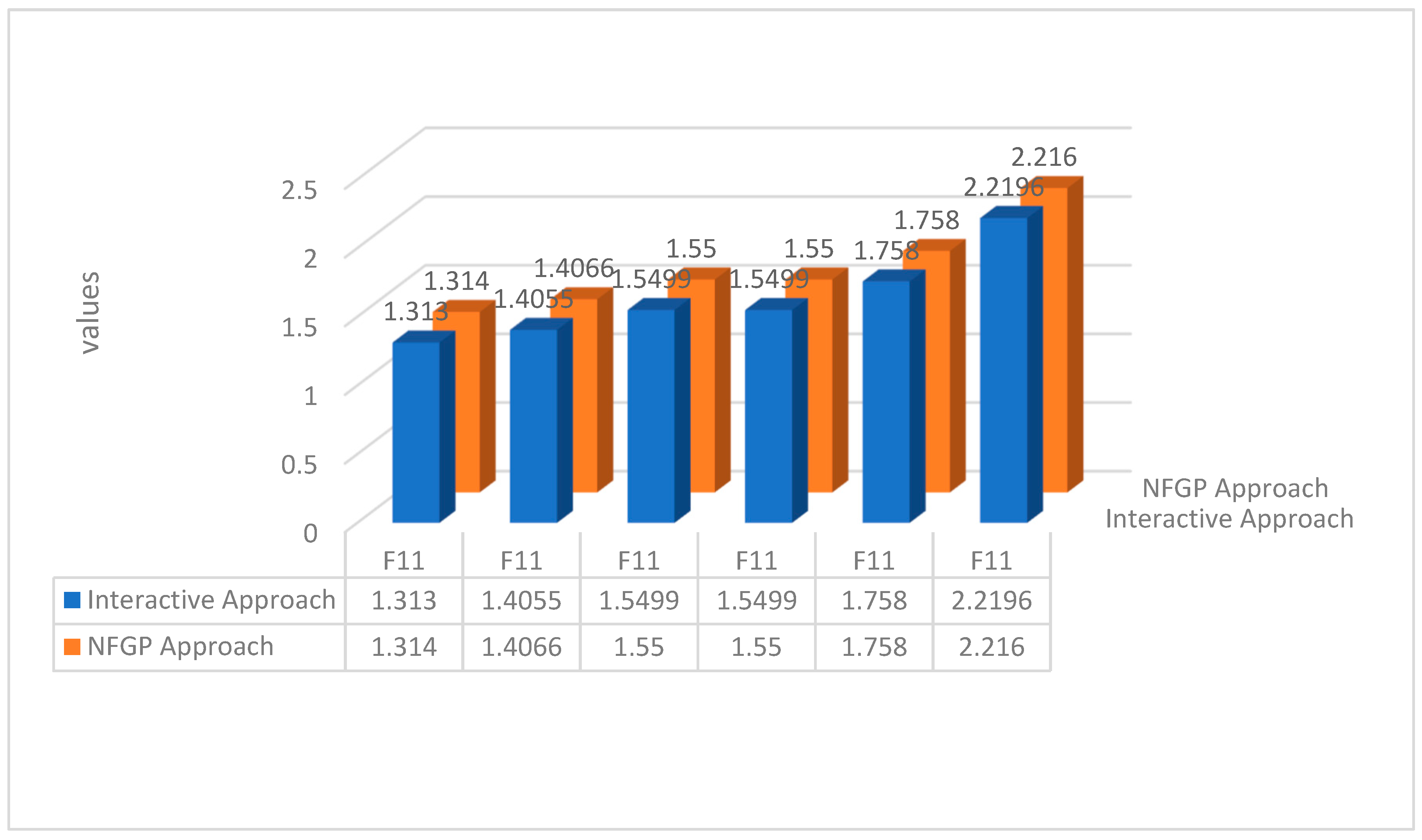
x 1 1 , x 1 2 , x 1 3 ; x 1 1 , x 1 2 , x 1 3 x 2 1 , x 2 2 , x 2 3 ; x 2 1 , x 2 2 , x 2 3 x 3 1 , x 3 2 , x 3 3 ; x 3 1 , x 3 2 , x 3 3 = 1.3989 ,   1.3989 ,   1.6842 ; 1.3989 ,   1.3989 ,   2.0497 1.6329 ,   1.6329 ,   1.9659 ; 1.6329 ,   1.6329 ,   2.3926 0.14096 ,   0.14096 ,   0.1697 ; 0.14096 ,   0.14096 ,   0.2065 f ~ 11 I = 1.4055 ,   1.5499 ,   1.758 ; 1.313 ,   1.5499 ,   2.2196
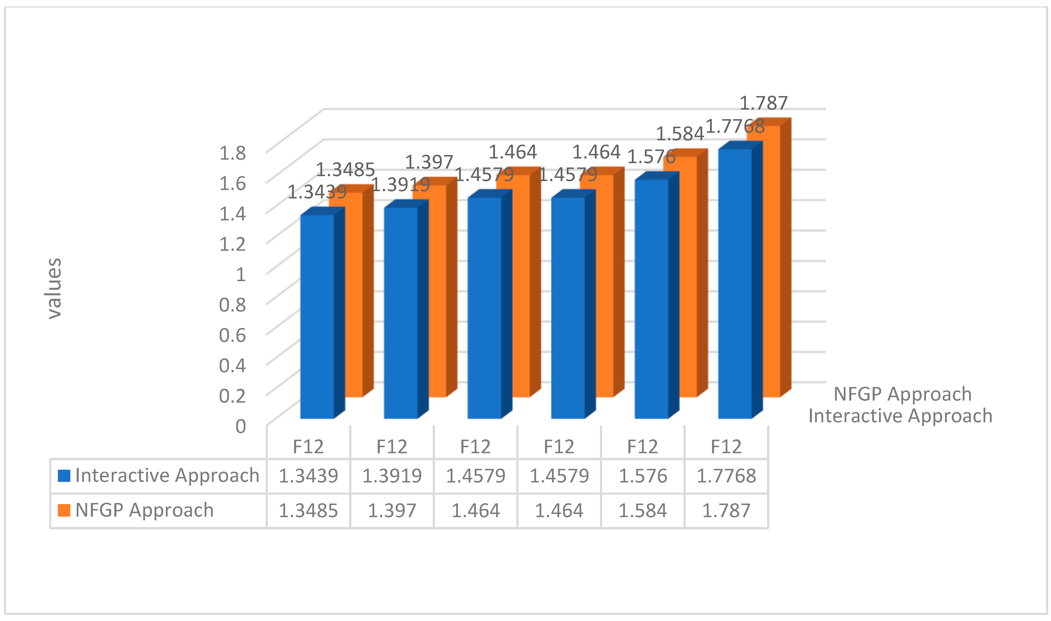
f ~ 12 I = 1.3919 ,   1.4579 ,   1.576 ; 1.3439 ,   1.4579 ,   1.7768
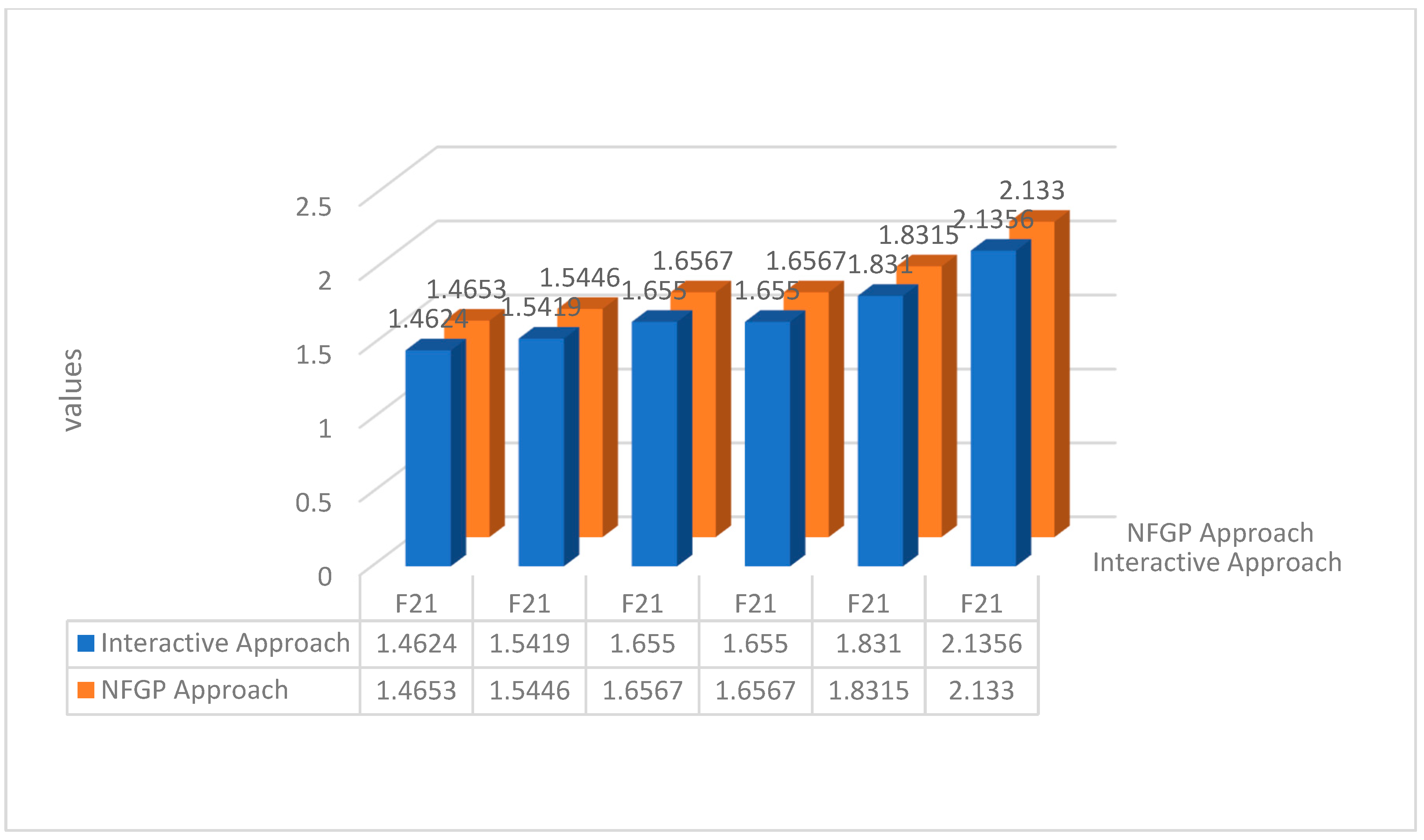
f ~ 21 I = 1.5489 ,   1.6545 ,   1.831 ; 1.4624 ,   1.6545 ,   2.1356
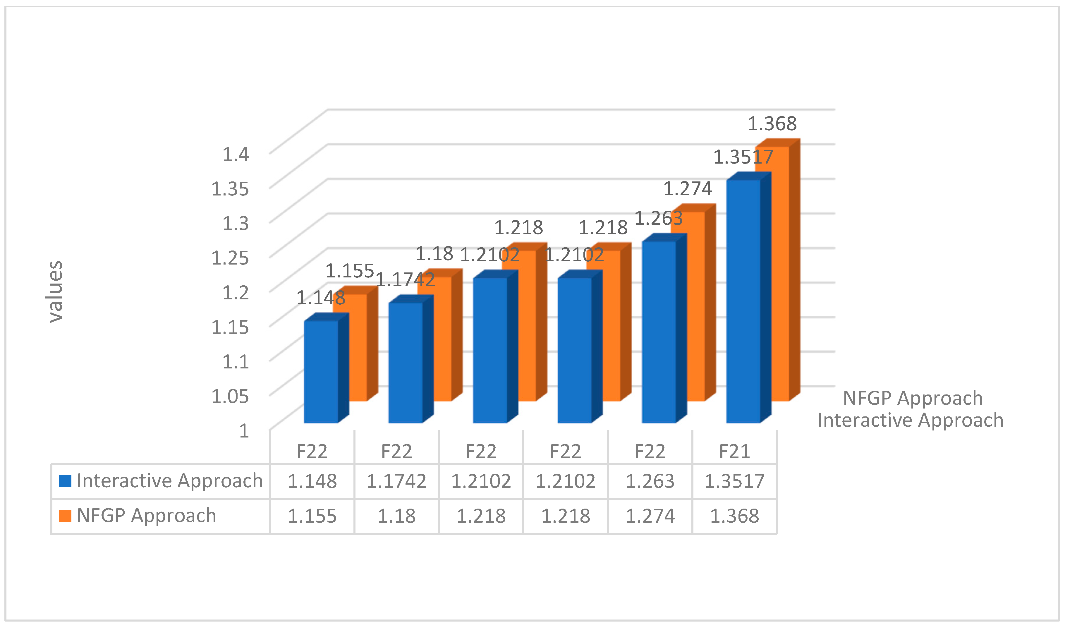
f ~ 22 I = 1.1742 ,   1.2102 ,   1.263 ; 1.148 ,   1.2102 ,   1.3517
f ~ 31 I = 1.7152 ,   1.8555   , 2.0855 ; 1.6158 ,   1.8555 ,   2.4844
f ~ 32 I = 1.3713 ,   1.4738 ,   1.5931 ; 1.2985 ,   1.4738 ,   1.793

7.2. Solution Based on NFGP Approach

Firstly, the FLDM NFGP model is formulated as follows:
m i n   Z = d 11 μ + d 12 μ + d 11 λ + d 12 λ + d 11 υ + + d 12 υ +
subject to
1 8 2 ω 1 1 + 6 ω 1 2 + 4 ω 1 3 + ω 1 1 + 6 ω 1 2 + 5 ω 1 3 + 5 ω 2 1 + 12 ω 2 2 + 7 ω 2 3 + 4 ω 2 1 + 12 ω 2 2 + 8 ω 2 3 + 3 ω 3 1 + 8 ω 3 2 + 5 ω 3 3 + 2 ω 3 1 + 8 ω 3 2   + 6 ω 3 3 + 8 t 1 + 18 t 2 + 10 t 3 + 7 t 1 + 18 t 2 + 11 t 3   0.000158 0.7944 0.000158 + d 11 μ d 11 μ + = 1 ,
1 8 2 ω 1 1 + 6 ω 1 2 + 4 ω 1 3 + ω 1 1 + 6 ω 1 2 + 5 ω 1 3 + 5 ω 2 1 + 12 ω 2 2 + 7 ω 2 3 + 4 ω 2 1 + 12 ω 2 2 + 8 ω 2 3 + 3 ω 3 1 + 8 ω 3 2 + 5 ω 3 3 + 2 ω 3 1 + 8 ω 3 2   + 6 ω 3 3 + 8 t 1 + 18 t 2 + 10 t 3 + 7 t 1 + 18 t 2 + 11 t 3   000158 0.7944 000158 + d 11 λ d 11 λ + = 0.5 ,
0.7944 1 8 2 ω 1 1 + 6 ω 1 2 + 4 ω 1 3 + ω 1 1 + 6 ω 1 2 + 5 ω 1 3 + 5 ω 2 1 + 12 ω 2 2 + 7 ω 2 3 + 4 ω 2 1 + 12 ω 2 2 + 8 ω 2 3 + 3 ω 3 1 + 8 ω 3 2 + 5 ω 3 3 + 2 ω 3 1 + 8 ω 3 2   + 6 ω 3 3 + 8 t 1 + 18 t 2 + 10 t 3 + 7 t 1 + 18 t 2 + 11 t 3   0.7944 000158 + d 11 υ d 11 υ + = 0 ,
1 8 3 ω 1 1 + 8 ω 1 2 + 5 ω 1 3 + 2 ω 1 1 + 8 ω 1 2 + 6 ω 1 3 + 9 ω 2 1 + 20 ω 2 2 + 11 ω 2 3 + 8 ω 2 1 + 20 ω 2 2 + 12 ω 2 3 + 4 ω 3 1 + 10 ω 3 2 + 6 ω 3 3 + 3 ω 3 1 + 10 ω 3 2   + 7 ω 3 3 + 6 t 1 + 14 t 2 + 8 t 3 + 5 t 1 + 14 t 2 + 9 t 3   0.000161 1.026 0.000161 + d 12 μ d 12 μ + = 1 ,
1 8 3 ω 1 1 + 8 ω 1 2 + 5 ω 1 3 + 2 ω 1 1 + 8 ω 1 2 + 6 ω 1 3 + 9 ω 2 1 + 20 ω 2 2 + 11 ω 2 3 + 8 ω 2 1 + 20 ω 2 2 + 12 ω 2 3 + 4 ω 3 1 + 10 ω 3 2 + 6 ω 3 3 + 3 ω 3 1 + 10 ω 3 2   + 7 ω 3 3 + 6 t 1 + 14 t 2 + 8 t 3 + 5 t 1 + 14 t 2 + 9 t 3   0.000161 1.026 0.000161 + d 12 λ d 12 λ + = 0.5 ,
  1.026 1 8 3 ω 1 1 + 8 ω 1 2 + 5 ω 1 3 + 2 ω 1 1 + 8 ω 1 2 + 6 ω 1 3 + 9 ω 2 1 + 20 ω 2 2 + 11 ω 2 3 + 8 ω 2 1 + 20 ω 2 2 + 12 ω 2 3 + 4 ω 3 1 + 10 ω 3 2 + 6 ω 3 3 + 3 ω 3 1 + 10 ω 3 2   + 7 ω 3 3 + 6 t 1 + 14 t 2 + 8 t 3 + 5 t 1 + 14 t 2 + 9 t 3   1.026 0.000161 + d 12 υ d 12 υ + = 0 ,
d i j × d i j + = 0 , a n d d i j , d i j + 0 , i = 1 , j = 1,2
ω 1 F , ω 2 S , , ω ( k 1 ) ( k 1 ) , ω k , t S ω , t
Using the Lingo 19 programming software, the FLDM’s satisfactory solution was ascertained as follows:
ω 1 1 , ω 1 2 , ω 1 3 ; ω 1 1 , ω 1 2 , ω 1 3 ω 2 1 , ω 2 2 , ω 2 3 ; ω 2 1 , ω 2 2 , ω 2 3 ω 3 1 , ω 3 2 , ω 3 3 ; ω 3 1 , ω 3 2 , ω 3 3 t 1 , t 2 , t 3 ; t 1 , t 2 , t 3 F = 0.04527 , 0.04527 , 0.04527 ; 0.04527 , 0.04527 , 0.04527 0.063017 , 0.063017 , 0.063017 ; 0.063017 , 0.063017 , 0.063017 0.00055 , 0.00055 , 0.00055 ; 0.00055 , 0.00055 , 0.00055 0.02447 ,   0.02949 , 0.03529 ; 0.02008 ,   0.02949 , 0.03529
The final NFGP model of the FIF-MLMOFPP is formulated as follows:
m i n   Z = d 11 μ + d 12 μ + d 21 μ + d 22 μ + d 31 μ + d 32 μ + d 11 λ + d 12 λ + d 21 λ + d 22 λ + d 31 λ + d 32 λ + d 11 υ + + d 12 υ + + d 21 υ + + d 22 υ + + d 31 υ + + d 32 υ +
subject to
1 8 2 ω 1 1 + 6 ω 1 2 + 4 ω 1 3 + ω 1 1 + 6 ω 1 2 + 5 ω 1 3 + 5 ω 2 1 + 12 ω 2 2 + 7 ω 2 3 + 4 ω 2 1 + 12 ω 2 2 + 8 ω 2 3 + 3 ω 3 1 + 8 ω 3 2 + 5 ω 3 3 + 2 ω 3 1 + 8 ω 3 2   + 6 ω 3 3 + 8 t 1 + 18 t 2 + 10 t 3 + 7 t 1 + 18 t 2 + 11 t 3   0.000158 0.7944 0.000158 + d 11 μ d 11 μ + = 1 ,
1 8 2 ω 1 1 + 6 ω 1 2 + 4 ω 1 3 + ω 1 1 + 6 ω 1 2 + 5 ω 1 3 + 5 ω 2 1 + 12 ω 2 2 + 7 ω 2 3 + 4 ω 2 1 + 12 ω 2 2 + 8 ω 2 3 + 3 ω 3 1 + 8 ω 3 2 + 5 ω 3 3 + 2 ω 3 1 + 8 ω 3 2   + 6 ω 3 3 + 8 t 1 + 18 t 2 + 10 t 3 + 7 t 1 + 18 t 2 + 11 t 3   000158 0.7944 000158 + d 11 λ d 11 λ + = 0.5 ,
0.7944 1 8 2 ω 1 1 + 6 ω 1 2 + 4 ω 1 3 + ω 1 1 + 6 ω 1 2 + 5 ω 1 3 + 5 ω 2 1 + 12 ω 2 2 + 7 ω 2 3 + 4 ω 2 1 + 12 ω 2 2 + 8 ω 2 3 + 3 ω 3 1 + 8 ω 3 2 + 5 ω 3 3 + 2 ω 3 1 + 8 ω 3 2   + 6 ω 3 3 + 8 t 1 + 18 t 2 + 10 t 3 + 7 t 1 + 18 t 2 + 11 t 3   0.7944 000158 + d 11 υ d 11 υ + = 0 ,
1 8 3 ω 1 1 + 8 ω 1 2 + 5 ω 1 3 + 2 ω 1 1 + 8 ω 1 2 + 6 ω 1 3 + 9 ω 2 1 + 20 ω 2 2 + 11 ω 2 3 + 8 ω 2 1 + 20 ω 2 2 + 12 ω 2 3 + 4 ω 3 1 + 10 ω 3 2 + 6 ω 3 3 + 3 ω 3 1 + 10 ω 3 2   + 7 ω 3 3 + 6 t 1 + 14 t 2 + 8 t 3 + 5 t 1 + 14 t 2 + 9 t 3   0.000161 1.026 0.000161 + d 12 μ d 12 μ + = 1 ,
1 8 3 ω 1 1 + 8 ω 1 2 + 5 ω 1 3 + 2 ω 1 1 + 8 ω 1 2 + 6 ω 1 3 + 9 ω 2 1 + 20 ω 2 2 + 11 ω 2 3 + 8 ω 2 1 + 20 ω 2 2 + 12 ω 2 3 + 4 ω 3 1 + 10 ω 3 2 + 6 ω 3 3 + 3 ω 3 1 + 10 ω 3 2   + 7 ω 3 3 + 6 t 1 + 14 t 2 + 8 t 3 + 5 t 1 + 14 t 2 + 9 t 3   0.000161 1.026 0.000161 + d 12 λ d 12 λ + = 0.5 ,
  1.026 1 8 3 ω 1 1 + 8 ω 1 2 + 5 ω 1 3 + 2 ω 1 1 + 8 ω 1 2 + 6 ω 1 3 + 9 ω 2 1 + 20 ω 2 2 + 11 ω 2 3 + 8 ω 2 1 + 20 ω 2 2 + 12 ω 2 3 + 4 ω 3 1 + 10 ω 3 2 + 6 ω 3 3 + 3 ω 3 1 + 10 ω 3 2   + 7 ω 3 3 + 6 t 1 + 14 t 2 + 8 t 3 + 5 t 1 + 14 t 2 + 9 t 3   1.026 0.000161 + d 12 υ d 12 υ + = 0 ,
1 8 4 ω 1 1 + 10 ω 1 2 + 6 ω 1 3 + 3 ω 1 1 + 10 ω 1 2 + 7 ω 1 3 + 9 ω 2 1 + 20 ω 2 2 + 11 ω 2 3 + 8 ω 2 1 + 20 ω 2 2 + 12 ω 2 3 + 8 ω 3 1 + 18 ω 3 2 + 10 ω 3 3 + 7 ω 3 1 + 18 ω 3 2   + 11 ω 3 3 + 7 t 1 + 16 t 2 + 9 t 3 + 6 t 1 + 16 t 2 + 10 t 3   0.000194 1.139 0.000194 + d 21 μ d 21 μ + = 1 ,
1 8 4 ω 1 1 + 10 ω 1 2 + 6 ω 1 3 + 3 ω 1 1 + 10 ω 1 2 + 7 ω 1 3 + 9 ω 2 1 + 20 ω 2 2 + 11 ω 2 3 + 8 ω 2 1 + 20 ω 2 2 + 12 ω 2 3 + 8 ω 3 1 + 18 ω 3 2 + 10 ω 3 3 + 7 ω 3 1 + 18 ω 3 2   + 11 ω 3 3 + 7 t 1 + 16 t 2 + 9 t 3 + 6 t 1 + 16 t 2 + 10 t 3   000194 1.139 000194 + d 21 λ d 21 λ + = 0.5 ,
1.139 1 8 4 ω 1 1 + 10 ω 1 2 + 6 ω 1 3 + 3 ω 1 1 + 10 ω 1 2 + 7 ω 1 3 + 9 ω 2 1 + 20 ω 2 2 + 11 ω 2 3 + 8 ω 2 1 + 20 ω 2 2 + 12 ω 2 3 + 8 ω 3 1 + 18 ω 3 2 + 10 ω 3 3 + 7 ω 3 1 + 18 ω 3 2   + 11 ω 3 3 + 7 t 1 + 16 t 2 + 9 t 3 + 6 t 1 + 16 t 2 + 10 t 3   1.139 000194 + d 21 υ d 21 υ + = 0 ,
1 8 8 ω 1 1 + 18 ω 1 2 + 10 ω 1 3 + 7 ω 1 1 + 18 ω 1 2 + 11 ω 1 3 + 3 ω 2 1 + 8 ω 2 2 + 5 ω 2 3   + 2 ω 2 1 + 8 ω 2 2 + 6 ω 2 3 + 6 ω 3 1 + 14 ω 3 2 + 8 ω 3 3 + 5 ω 3 1 + 14 ω 3 2 + 9 ω 3 3 + 4 t 1 + 10 t 2 + 6 t 3 + 3 t 1 + 10 t 2 + 7 t 3   0.000227 0.9954 0.000227 + d 22 μ d 22 μ + = 1 ,
1 8 8 ω 1 1 + 18 ω 1 2 + 10 ω 1 3 + 7 ω 1 1 + 18 ω 1 2 + 11 ω 1 3 + 3 ω 2 1 + 8 ω 2 2 + 5 ω 2 3   + 2 ω 2 1 + 8 ω 2 2 + 6 ω 2 3 + 6 ω 3 1 + 14 ω 3 2 + 8 ω 3 3 + 5 ω 3 1 + 14 ω 3 2 + 9 ω 3 3 + 4 t 1 + 10 t 2 + 6 t 3 + 3 t 1 + 10 t 2 + 7 t 3   0.000227 0.9954 0.000227 + d 22 λ d 22 λ + = 0.5 ,
0.9954 1 8 8 ω 1 1 + 18 ω 1 2 + 10 ω 1 3 + 7 ω 1 1 + 18 ω 1 2 + 11 ω 1 3 + 3 ω 2 1 + 8 ω 2 2 + 5 ω 2 3   + 2 ω 2 1 + 8 ω 2 2 + 6 ω 2 3 + 6 ω 3 1 + 14 ω 3 2 + 8 ω 3 3 + 5 ω 3 1 + 14 ω 3 2 + 9 ω 3 3 + 4 t 1 + 10 t 2 + 6 t 3 + 3 t 1 + 10 t 2 + 7 t 3   0.9954 0.000227 + d 22 υ d 22 υ + = 0 ,
1 8 5 ω 1 1 + 12 ω 1 2 + 7 ω 1 3 + 4 ω 1 1 + 12 ω 1 2 + 8 ω 1 3 + 11 ω 2 1 + 24 ω 2 2 + 13 ω 2 3   + 10 ω 2 1 + 24 ω 2 2 + 14 ω 2 3 + 3 ω 3 1 + 8 ω 3 2 + 5 ω 3 3 + 2 ω 3 1 + 8 ω 3 2 + 6 ω 3 3 + 7 t 1 + 16 t 2 + 9 t 3 + 6 t 1 + 16 t 2 + 10 t 3   0.000199 1.271 0.000199 + d 31 μ d 31 μ + = 1 ,
1 8 5 ω 1 1 + 12 ω 1 2 + 7 ω 1 3 + 4 ω 1 1 + 12 ω 1 2 + 8 ω 1 3 + 11 ω 2 1 + 24 ω 2 2 + 13 ω 2 3   + 10 ω 2 1 + 24 ω 2 2 + 14 ω 2 3 + 3 ω 3 1 + 8 ω 3 2 + 5 ω 3 3 + 2 ω 3 1 + 8 ω 3 2 + 6 ω 3 3 + 7 t 1 + 16 t 2 + 9 t 3 + 6 t 1 + 16 t 2 + 10 t 3   0.000199 1.271 0.000199 + d 31 λ d 31 λ + = 0.5 ,
1.271 1 8 5 ω 1 1 + 12 ω 1 2 + 7 ω 1 3 + 4 ω 1 1 + 12 ω 1 2 + 8 ω 1 3 + 11 ω 2 1 + 24 ω 2 2 + 13 ω 2 3   + 10 ω 2 1 + 24 ω 2 2 + 14 ω 2 3 + 3 ω 3 1 + 8 ω 3 2 + 5 ω 3 3 + 2 ω 3 1 + 8 ω 3 2 + 6 ω 3 3 + 7 t 1 + 16 t 2 + 9 t 3 + 6 t 1 + 16 t 2 + 10 t 3   1.271 0.000199 + d 31 υ d 31 υ + = 0 ,
1 8 3 ω 1 1 + 8 ω 1 2 + 5 ω 1 3 + 2 ω 1 1 + 8 ω 1 2 + 6 ω 1 3 + 6 ω 2 1 + 14 ω 2 2 + 8 ω 2 3 + 5 ω 2 1 + 14 ω 2 2 + 9 ω 2 3 + 10 ω 3 1 + 22 ω 3 2 + 12 ω 3 3 + 9 ω 3 1 + 22 ω 3 2 + 13 ω 3 3 + 11 t 1 + 24 t 2 + 13 t 3 + 10 t 1 + 24 t 2 + 13 t 3   0.000211 1.176 0.000211 + d 32 μ d 32 μ + = 1 ,
1 8 3 ω 1 1 + 8 ω 1 2 + 5 ω 1 3 + 2 ω 1 1 + 8 ω 1 2 + 6 ω 1 3 + 6 ω 2 1 + 14 ω 2 2 + 8 ω 2 3 + 5 ω 2 1 + 14 ω 2 2 + 9 ω 2 3 + 10 ω 3 1 + 22 ω 3 2 + 12 ω 3 3 + 9 ω 3 1 + 22 ω 3 2 + 13 ω 3 3 + 11 t 1 + 24 t 2 + 13 t 3 + 10 t 1 + 24 t 2 + 13 t 3   0.000211 1.176 0.000211 + d 32 λ d 32 λ + = 0.5 ,
1.176 1 8 3 ω 1 1 + 8 ω 1 2 + 5 ω 1 3 + 2 ω 1 1 + 8 ω 1 2 + 6 ω 1 3 + 6 ω 2 1 + 14 ω 2 2 + 8 ω 2 3 + 5 ω 2 1 + 14 ω 2 2 + 9 ω 2 3 + 10 ω 3 1 + 22 ω 3 2 + 12 ω 3 3 + 9 ω 3 1 + 22 ω 3 2 + 13 ω 3 3 + 11 t 1 + 24 t 2 + 13 t 3 + 10 t 1 + 24 t 2 + 13 t 3   1.176 0.000211 + d 32 υ d 32 υ + = 0 ,
ω 1 1 , ω 1 2 , ω 1 3 ; ω 1 1 , ω 1 2 , ω 1 3 F = 0.04527,0.04527,0.04527 ; 0.04527,0.04527,0.04527
ω 2 1 , ω 2 2 , ω 2 3 ; ω 2 1 , ω 2 2 , ω 2 3 S = 0.05619,0.05619,0.05619 ; 0.05619,0.05619,0.05619
d i j × d i j + = 0 ,   a n d   d i j ,   d i j + 0 ,   i = 1,2 , 3   j = 1,2
ω 3 , t S ω , t
The final satisfactory solution for the NFGP model of the FIF-MLMOFPP is obtained as follows:
ω 1 1 , ω 1 2 , ω 1 3 ; ω 1 1 , ω 1 2 , ω 1 3 F ω 2 1 , ω 2 2 , ω 2 3 ; ω 2 1 , ω 2 2 , ω 2 3 S ω 3 1 , ω 3 2 , ω 3 3 ; ω 3 1 , ω 3 2 , ω 3 3 T t 1 , t 2 , t 3 ; t 1 , t 2 , t 3 = 0.04527 , 0.04527 , 0.04527 ; 0.04527 , 0.04527 , 0.04527 0.05619 , 0.05619 , 0.05619 ; 0.05619 , 0.05619 , 0.05619 0.006949 , 0.006949 , 0.006949 ; 0.006949 , 0.006949 , 0.006949 0.02855 ,   0.034064 , 0.034064 ; 0.023279 ,   0.034064 , 0.034064
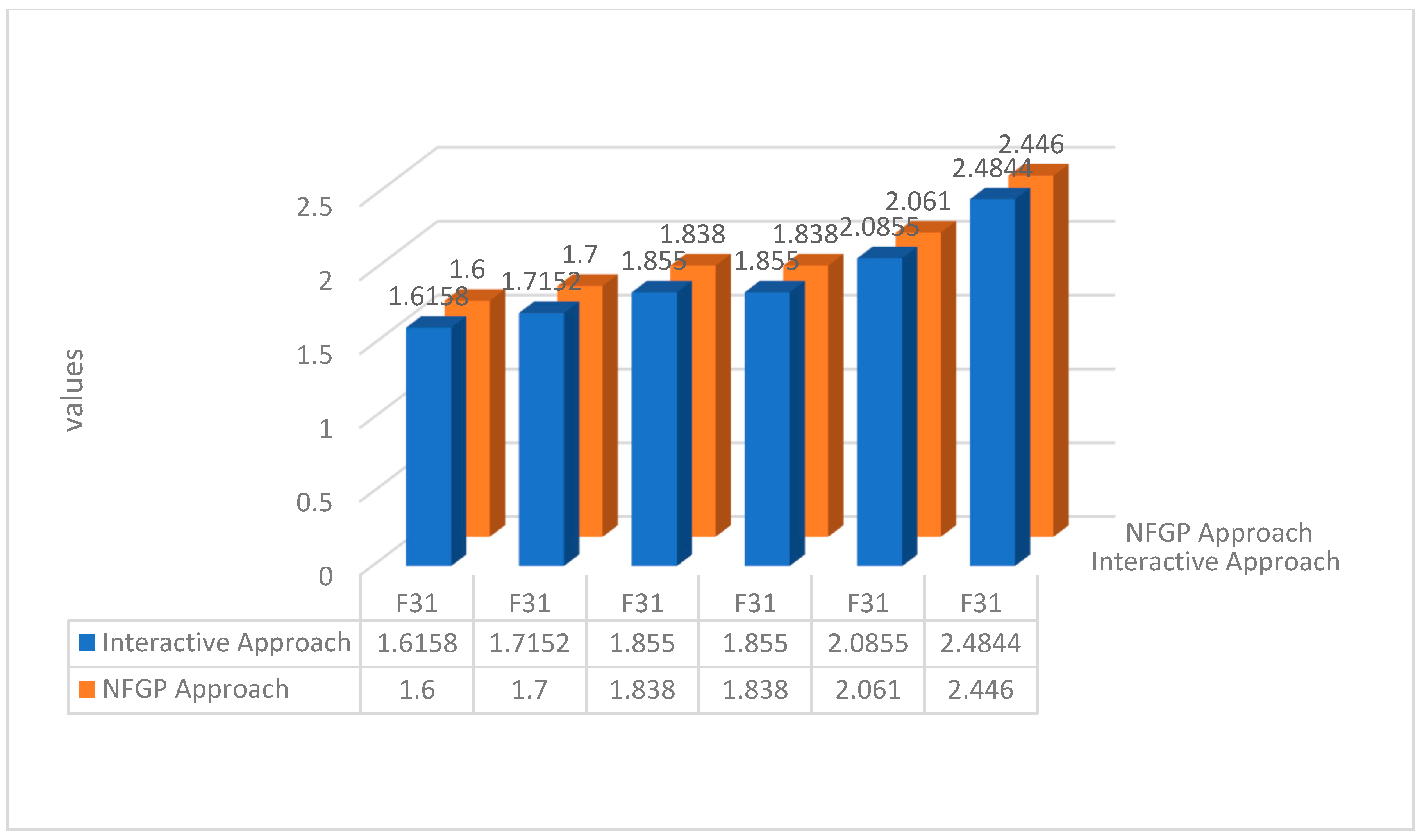
Figure 2, Figure 3, Figure 4, Figure 5, Figure 6 and Figure 7 present a comparison between the NFGP and the suggested interactive method. The findings indicate that the NFGP technique and the suggested interactive approach’s preferred solution are nearly identical.

8. Discussion

Both the interactive approach and the NFGP approach were utilized to solve the FIF-MLMOFPP, which has not been introduced in the literature before. The interactive approach is very effective, as it is mainly based on the ϵ -constraint method, which is a powerful technique for solving MOOPs at each level. Moreover, the interactive approach gives the DMs the ability to interact with the analysts to reach a satisfactory solution. The NFGP is a novel method for solving the FIF-MLMOFPP, as it is based on the goal programming technique within a neutrosophic fuzzy domain, where unwanted deviational variables are minimized. In the developed final model of the NFGP approach, linear membership and non-membership functions were utilized. Other types of membership functions, such as parabolic and hyperbolic membership functions, can be used, but the model will be more complicated.
To guarantee the suitability and computational effectiveness of the suggested models for resolving the FIF-MLMOFPP, numerical data for the interactive and NFGP approaches are displayed in Table 2. The elapsed runtimes per second for the two approaches are close to one another. The total number of solver iterations for the NFGP is smaller than that of the interactive approach. Additionally included are the model class, integer variables, nonlinear variables, and total number of constraints. Numerous organizations involved in supply chain networks and logistic systems can benefit greatly from the study that has been conducted here. Any real-world problem that can be modeled in a fully intuitionistic fuzzy fractional multi-level optimization will depend on the presented study. The two proposed approaches for FIF-MLMOFPP are straightforward to implement, making them accessible for educational purposes and practical applications.
The proposed approach offers several advantages when applied efficiently in both numerical problems and real-life applications.
-
The proposed multi-level fractional optimization modeling approach handles intuitionistic fuzzy parameters, which involve membership as well as non-membership functions and are more realistic compared to fuzzy parameters;
-
The proposed NFGP approach addresses the indeterminacy degree, which is the area of uncertainty between the acceptance and rejection degrees of propositions.
-
The proposed model is able to handle the FIF-MLMOFPP because it is a simple concept, easy to implement, requires less execution effort, and is more flexible and adaptive to a wide variety of problems.
-
It can be easily implemented in different real-life problems, such as transportation, supplier selection, supply chain, manufacturing, inventory control, assignment problems, etc.

9. Conclusions

A method for resolving the FIF-MLMOFPP is presented in this paper. A degree of non-membership, which is not merely the complement of the membership degree, can also be defined using the concept of an IFN environment. By comparing two IFNs and employing an accurate function, the problem was simplified to a deterministic fractional ML-MOOP. Using two different methods, a suitable solution for the FIF-MLMOFPP at each level was obtained. To obtain a good solution for the provided model, the interactive technique uses the ϵ -constraint method and satisfactoriness. Furthermore, by lowering their deviational variables, the NFGP approach is used to achieve the highest levels of each marginal evaluation goal and, as a result, obtain a satisfying solution. The introduced model’s primary benefit is that it offers an IFN that is satisfactory. Furthermore, the suggested model requires less computing work to produce a good solution and may be readily utilized in a variety of uncertain domains.
There are still a number of intriguing research directions in the field of FIF-MLMOFPP that need to be investigated. Future research could focus on the following areas:
-
Multi-choice rough fractional ML-MOOP models utilizing the interactive approach;
-
Fully intuitionistic fuzzy fractional bi-level production planning models;
-
Intuitionistic fuzzy bi-level supply chain models using the NFGP approach.

Author Contributions

Conceptualization, M.A.E.S.; Methodology, H.E. and M.A.E.S.; Software, F.A.F. and M.A.E.S.; Validation, M.A.E. and F.A.B.; Formal analysis, F.A.F., T.K. and J.H.; Investigation, H.E. and F.A.B.; Data curation, M.A.E. and M.A.E.S.; Writing—original draft, F.A.F. and H.E.; Writing—review and editing, M.A.E.S.; Supervision, J.H. and T.K.; Funding acquisition, M.A.E.S. All authors have read and agreed to the published version of the manuscript.

Funding

The authors would like to thank the Ongoing Research Funding Program (ORF-2025-1349), King Saud University, Riyadh, Saudi Arabia, for financial support.

Data Availability Statement

The data used to support the findings of this study are available from the corresponding author upon request.

Conflicts of Interest

The authors declare no conflicts of interest.

Abbreviations

FIF-MLMOFPPFully intuitionistic fuzzy multi-level multi-objective fractional programming problem
IFNsIntuitionistic fuzzy numbers
FIF-MLMOPPFully intuitionistic fuzzy multi-level multi-objective programming problem
MOOPMulti-objective optimization problem
NFGPNeutrosophic fuzzy goal programming
DMsDecision makers
ML-MOOPsMulti-level multi-objective optimization problems
FSTFuzzy set theory
FLDMFirst-level decision maker
BLOPsBi-level programming problems
FGPFuzzy goal programming
IFSIntuitionistic fuzzy sets
NSNeutosophic sets
TIFNTriangular intuitionistic fuzzy number
SLDMSecond-level decision maker
KLDMK-level decision maker
TOPSISTechnique of Order Preferences by Similarity to Ideal Solution

References

  1. Atanassov, K.T. Intuitionistic fuzzy sets. Fuzzy Sets Syst. 1986, 20, 87–96. [Google Scholar] [CrossRef]
  2. Singh, V.P.; Sharma, K.; Chakraborty, D.; Ebrahimnejad, A. A novel multi-objective bi-level programming problem under intuitionistic fuzzy environment and its application in production planning problem. Complex Intell. Syst. 2022, 8, 3263–3278. [Google Scholar] [CrossRef]
  3. Sharma, K.; Singh, V.P.; Ebrahimnejad, A.; Chakraborty, D. Solving a multi-objective chance constrained hierarchical optimization problem under intuitionistic fuzzy environment with its application. Expert Syst. Appl. 2023, 217, 119595. [Google Scholar] [CrossRef]
  4. Abo-Sinna, M.A.; Baky, I.A. Interactive balance space approach for solving multi-level multi-objective programming problems. Inf. Sci. 2007, 177, 3397–3410. [Google Scholar] [CrossRef]
  5. Abo-Elnagga, Y.; Elsisy, M.A.; El Sayed, M.A. A novel algorithm for generating Pareto frontier of bi-level multi-objective rough nonlinear programming problem. Ain Shams Eng. J. 2021, 12, 2125–2133. [Google Scholar]
  6. Baky, I.A. Solving multi-level multi-objective linear programming problems through fuzzy goal programming approach. Appl. Math. Model. 2010, 34, 2377–2387. [Google Scholar] [CrossRef]
  7. Osman, M.S.; Emam, O.E.; El Sayed, M.A. Interactive Approach for Multi-Level Multi-Objective Fractional Programming Problems with Fuzzy Parameters. Beni-Suef Univ. J. Basic Appl. Sci. 2018, 7, 139–149. [Google Scholar] [CrossRef]
  8. Pramanik, S.; Roy, T.K. Fuzzy goal programming approach to multi-level programming problems. Eur. J. Oper. Res. 2007, 176, 1151–1166. [Google Scholar] [CrossRef]
  9. Chen, L.H.; Chen, H.H. A two-phase fuzzy approach for solving multi-level decision-making problems. Knowl. Based Syst. 2015, 76, 189–199. [Google Scholar] [CrossRef]
  10. Lachhwani, K. Modified FGP approach for multi-level multi objective linear fractional programming problems. Appl. Math. Comput. 2015, 266, 1038–1049. [Google Scholar] [CrossRef]
  11. Osman, M.S.; Emam, O.E.; El Sayed, M.A. Stochastic fuzzy multi-level mutiobjective fractional programming problem: A FGP approach. OPSEARCH 2017, 54, 816–840. [Google Scholar] [CrossRef]
  12. Ren, A. A novel method for solving the fully fuzzy bi-level linear programming problem. Math. Prob. Eng. 2015, 2, 1–11. [Google Scholar]
  13. Baky, I.A. Fuzzy goal programming algorithm for solving decentralized bi-level multi-objective programming problems. Fuzzy Sets Systems 2009, 160, 2701–2713. [Google Scholar] [CrossRef]
  14. Baky, I.A.; Eid, M.H.; El Sayed, M.A. Bi-level multi-objective programming problem with fuzzy demands: A fuzzy goal programming algorithm. OPSEARCH 2014, 51, 280–296. [Google Scholar] [CrossRef]
  15. Arora, S.R.; Gupta, R. Interactive fuzzy goal programming approach for bi-level programming problem. Eur. J. Oper. Res. 2009, 194, 368–376. [Google Scholar] [CrossRef]
  16. Toksari, M.D.; Bilim, Y. Interactive fuzzy goal programming based on jacobian matrix to solve decentralized bi-level multi-objective fractional programming problems. Int. J. Fuzzy Syst. 2015, 17, 499–508. [Google Scholar] [CrossRef]
  17. Emam, O.E. Interactive approach to bi-level integer multi-objective fractional programming problem. Appl. Math. Comput. 2013, 233, 17–24. [Google Scholar] [CrossRef]
  18. Helmy, Y.M.; Emam, O.E.; Abdelwahab, A.M. On stochastic multi-level multiobjective fractional programming problems. J. Stat. Appl. Probab. 2015, 4, 93–101. [Google Scholar]
  19. El Sayed, M.A.; Baky, I.A.; Singh, P. A modified TOPSIS approach for solving stochastic fuzzy multi-level multi-objective fractional decision making problem. OPSEARCH 2020, 57, 1374–1403. [Google Scholar] [CrossRef]
  20. El Sayed, M.A.; Farahat, F.A.; Elsisy, M.A.; Alsabaan, M.; Ibrahem MIElwahsh, H. Two TOPSIS-Based Approaches for Multi-Choice Rough Bi-Level Multi-Objective Nonlinear Programming Problems. Mathematics 2025, 13, 1242. [Google Scholar] [CrossRef]
  21. Bhati, D.; Singh, P. Branch and bound computational method for multi-objective linear fractional optimization problem. Neural Comput. Appl. 2017, 28, 3341–3351. [Google Scholar] [CrossRef]
  22. AbdAlhakim, H.; Emam, O.E.; Abd El-Mageed, A.A. Architecting a fully fuzzy information model for multi-level quadratically constrained quadratic programming problem. OPSEARCH 2019, 56, 367–389. [Google Scholar] [CrossRef]
  23. Ahlatcioglu, M.; Tiryaki, F. Interactive fuzzy programming for decentralized two-level linear fractional programming problems. Omega 2007, 35, 432–450. [Google Scholar] [CrossRef]
  24. Emam, O.E.; El-Araby, M.; Belal, M.A. On Rough Multi-Level Linear Programming Problem. Inf. Sci. Lett. 2015, 4, 41–49. [Google Scholar]
  25. Nayak, S.; Ojha, A.K. An approach of fuzzy and TOPSIS to bi-level multi-objective nonlinear fractional programming problem. Soft Comput. 2019, 23, 5605–5618. [Google Scholar] [CrossRef]
  26. Abo-Sinna, M.A.; Amer, A.H. TOPSIS approach for solving bi-level non-linear fractional MODM problems. J. Adv. Math. 2018, 13, 7353–7370. [Google Scholar] [CrossRef]
  27. Guzel, N. A proposal to the solution of multi-objective linear fractional programming problem. Abstr. Appl. Anal. 2013, 2013, 435030. [Google Scholar] [CrossRef]
  28. Arya, R.; Singh, P.; Kumari, S.; Obaidat, M.S. An approach for solving fully fuzzy multi-objective linear fractional optimization problems. Soft Comput. 2019, 24, 9105–9119. [Google Scholar] [CrossRef]
  29. Angammal, S.; Hannah, G. A new bi-level TOPSIS based neutrosophic programming technique for land allocation to medium farm holders. Heliyon 2024, 10, e36166. [Google Scholar] [CrossRef]
  30. Ahmad, F.; Adhami, A.Y. Neutrosophic programming approach to multiobjective nonlinear transportation problem with fuzzy parameters. Int. J. Manag. Sci. Eng. Manag. 2019, 14, 218–229. [Google Scholar] [CrossRef]
  31. Ahmad, F.; Adhami, A.Y.; Smarandache, F. Single Valued Neutrosophic Hesitant Fuzzy Computational Algorithm for Multiobjective Nonlinear Optimization Problem. Neutrosophic Sets Syst. 2018, 22, 76–86. [Google Scholar]
  32. Smarandache, F. A Unifying Field in Logics: Neutrosophic Logic. In Philosophy; American Research Press: Champaign, IL, USA, 1999; pp. 1–141. [Google Scholar]
  33. Ahmad, F.; Adhami, A.Y.; Smarandache, F. Modified Neutrosophic Fuzzy Optimization Model for Optimal Closed-Loop Supply Chain Management Under Uncertainty. In Optimization Theory Based on Neutrosophic and Plithogenic Sets; Elsevier: Amsterdam, The Netherlands, 2020; pp. 343–403. [Google Scholar]
  34. Ahmad, S.; Ahmad, F.; Sharaf, M. Supplier selection problem with type-2 fuzzy parameters: A neutrosophic optimization approach. Int. J. Fuzzy Syst. 2021, 23, 755–775. [Google Scholar] [CrossRef]
  35. Almotairi, S.; Badr, E.; Elsisy, M.A.; Farahat, F.A.; El Sayed, M.A. Performance Analysis of Fully Intuitionistic Fuzzy Multi-Objective Multi-Item Solid Fractional Transportation Model. Fractal Fract. 2024, 8, 404. [Google Scholar] [CrossRef]
  36. Ahmad, F.; Ahmad, S.; Soliman, A.T.; Abdollahian, M. Solving multi-level multi-objective fractional programming problem with rough interval parameter in neutrosophic environment. RAIRO Oper. Res. 2021, 55, 2567–2581. [Google Scholar] [CrossRef]
  37. Ahmadini, A.A.H.; Ahmad, F. Solving intuitionistic fuzzy multiobjective linear programming problem under neutrosophic environment. AIMS Math. 2021, 6, 4556–4580. [Google Scholar] [CrossRef]
  38. Fathy, E.; Ammar, E.; Helmy, M.A. Fully intuitionistic fuzzy multi-level linear fractional programming problem. Alex. Eng. J. 2023, 77, 684–694. [Google Scholar] [CrossRef]
  39. El Sayed, M.A.; Abo-Sinna, M.A. A novel Approach for Fully Intuitionistic Fuzzy Multi-Objective Fractional Transportation Problem. Alex. Eng. J. 2021, 60, 1447–1463. [Google Scholar] [CrossRef]
  40. Mahajan, S.; Chauhan, A.; Gupta, S.K. On Pareto optimality using novel goal programming approach for fully intuitionistic fuzzy multiobjective quadratic problems. Expert Syst. Appl. 2024, 243, 122816. [Google Scholar] [CrossRef]
  41. Roy, S.K.; Ebrahimnejad, A.; Verdegay, J.L.; Das, S. New approach for solving intuitionistic fuzzy multi-objective transportation problem. Sadhana 2018, 43, 3. [Google Scholar] [CrossRef]
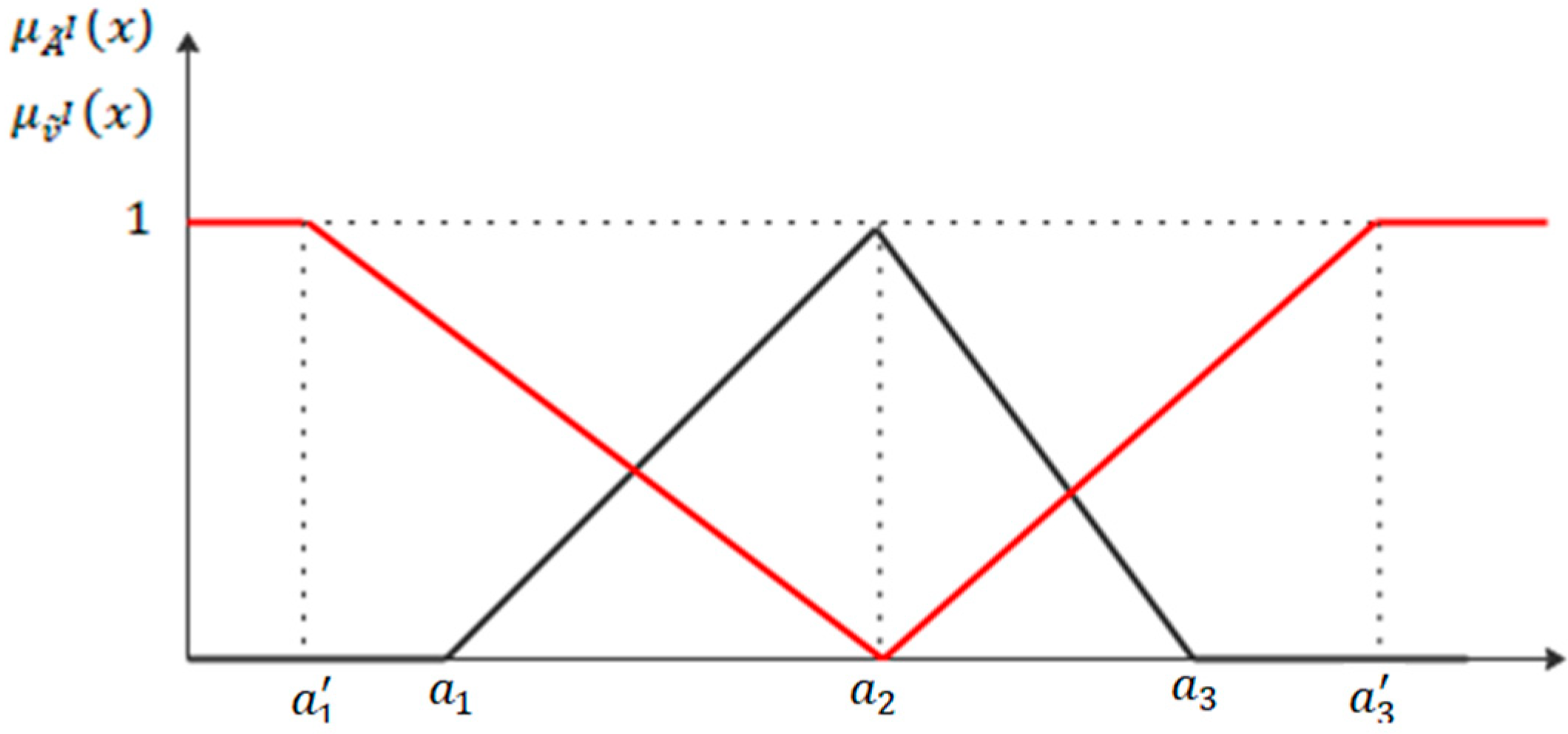
Figure 1. Triangular intuitionistic fuzzy number.
Fractalfract 09 00675 g001
Figure 2. Intuitionistic fuzzy values of f 11 x .
Fractalfract 09 00675 g002
Figure 3. Intuitionistic fuzzy values of f 12 ( x ) .
Fractalfract 09 00675 g003
Figure 4. Intuitionistic fuzzy values of f 21 ( x ) .
Fractalfract 09 00675 g004
Figure 5. Intuitionistic fuzzy values of f 22 ( x ) .
Fractalfract 09 00675 g005
Figure 6. Intuitionistic fuzzy values of f 31 ( x ) .
Fractalfract 09 00675 g006
Figure 7. Intuitionistic fuzzy values of f 32 ( x ) .
Fractalfract 09 00675 g007
Table 1. Individual maximum and minimum values.
R 11 ( ω , t ) R 12 ( ω , t ) R 21 ( ω , t ) R 22 ( ω , t ) R 31 ( ω , t ) R 32 ( ω , t )
b i j = m a x ( R i j ( ω , t ) ) 0.79441.0261.1390.99541.2711.1759
a i j = m i n ( R i j ω , t ) 0.0001580.0001610.0001940.0002270.0001990.000211
Table 2. Numerical data of interactive approach and NFGP approach.
Interactive ApproachNFGP Approach
Total solver iteration2016
Elapsed runtime seconds0.100.13
Model classLPLP
Total variables1252
Nonlinear variables00
Integer variables00
Total constraints68107
Disclaimer/Publisher’s Note: The statements, opinions and data contained in all publications are solely those of the individual author(s) and contributor(s) and not of MDPI and/or the editor(s). MDPI and/or the editor(s) disclaim responsibility for any injury to people or property resulting from any ideas, methods, instructions or products referred to in the content.