Abstract
In this work, the advection-dispersion model (ADM) is time-fractionalized by the exploitation of Atangana-Baleanu (AB) differential operator to describe contaminant transport in a geological environment. Dispersion, adsorption, and decay, which are known as the foremost transport mechanisms, are considered. The exact solutions of the suggested Atangana-Baleanu advection-dispersion models (AB-ADMs) are acquired using Fourier sine transform and Laplace transform. The classical ADMs are demonstrated to be the special limiting cases of the suggested models. The high consistency among the suggested models and experimental data denotes that the AB-ADMs characterize contaminant transport more effectively. Additionally, the corresponding numerical and graphical results are explored to demonstrate the necessity, effectiveness, and suitability of the suggested models.
Keywords:
Atangana-Baleanu differential operator; advection-dispersion; contaminant transport; adsorption; first-order decay MSC:
26A33; 35R11; 44A10; 47A62; 74S40
1. Introduction
Efforts to inhibit or even prevent the migration of a contaminant through the geological system have always been the focus of safe treatment and disposal of contaminants. Researchers with diverse backgrounds in hydrology, geology, soil science, engineering, physics, chemistry, statistics, and mathematics have undertaken a broad range of theoretical, numerical, laboratory, and field investigations [1]. Many issues focusing on migration of contaminants have been addressed, from a variety of perspectives. It is found that, due to the complex contaminant migration mechanism, the diversity of surrounding rock selection, the heterogeneity of geological body, the complexity and variability of groundwater flow field, and so on, multiple mechanisms, including convection, dispersion, adsorption, and decay, need to be considered in the establishment of contaminant diffusion models [2], which means the analytical solutions of solute transport models considering multiple mechanisms are expressed in more complicated forms [3]. Then, it is a key point to establish the contaminant transport models to portray the process of contaminant transport more accurately. At the same time, the experimental research on the migration of a contaminant is in progress; Ajayi et al. [4] and Krsti et al. [5] investigated the vertical distribution of Cesium in soil. Pang and Casey et al. [6,7] discussed the solute transport with sorption and degradation, while Chen et al. [8,9] studied the migration of radionuclides in granite. A great deal of experimental studies indicated that the contaminant migration in porous media reveals a long-tail phenomenon [10,11,12], which cannot be captured via the traditional contaminant transport models. As a result, the improvement of contaminant transport models is necessary.
On the other hand, the fractional derivative [13] emerged as an idea of generalization of the classical derivative definition, and it has become a key tool in engineering modeling [14,15,16,17]. The non-locality property of the fractional derivative makes problems fractionalized so that they are more functional and precise in relation to the classical cases, and it turned out to yield obvious advantages in describing the long-tail phenomenon and time-dependence characteristics [18,19]. Convincing evidence in much literature has shown that the typical deviations from classical ADM (power-law decay in breakthrough curves) can be amended by introducing fractional operators. The well-known fractional derivative definition, the Caputo derivative [20], has wide applications in many fields, such as non-Darcian flow [21], contaminant transport [22], and the viscoelastic model and diffusion [23,24], due to the fact that the Caputo derivative is not necessary to define fractional-order initial conditions when solving the differential equations. Unlike the Caputo derivative definition based on power-law kernel with singularity; in the last decade, some new non-singular differential operators have been proposed. Caputo and Fabrizio [25] proposed a differential operator with an exponential kernel. The Caputo–Fabrizio differential operator has been employed in a number of areas, for instance, fluid flow [26,27], the virus model [28,29], and the human liver model [30]. Recently, Atangana and Baleanu [31] put forward a new non-local and non-singular fractional operator employing the Mittag–Leffler function as its kernel, which aims to describe the full memory effect in systems since the Mittag–Leffler function features exponential and power-law decay at short and long time scales, respectively. It is widely used to describe real-world problems [32,33,34,35,36].
The diffusion model is the basic and classical model for describing solute transport. In order to describe a realistic transport phenomenon in a geological system, the solute transport models in porous media usually consider diffusion, advection, and other reactions. Apart from the diffusion model forms, the continuous-time random walk model [37], which is often discussed in physics, the multirate mass transfer model [38], fractional mobile–immobile models [39], and stochastic streamtube approaches [40] are frequently used in the literature. Considering first-order decay, adsorption, and advection to the diffusion model of the contaminant, which is also called the advection–dispersion model (ADM), the objective of this work is expected to provide generalized models of contaminant migration in geological environment associated with the Atangana–Baleanu (AB) differential operator to develop and analytically solve AB-fractional advection–dispersion equations with adsorption and decay and to validate them against benchmark experimental datasets. The relative experimental data are used to fit the obtained analytical solution, and the corresponding numerical pictures give a clear description of the results shown in this work. The commonly used solutions of ADM are shown to be the special cases of the proposed model.
The rest of this work is organized as follows. In Section 2, the advection–dispersion model with Atangana–Baleanu differential operator (AB-ADM) is proposed. In Section 3 and Section 4, the AB-ADMs with linear adsorption and first-order decay for describing contaminant transport are introduced, respectively, and the accurate analytical solutions are obtained. Moreover, the related experimental data are displayed to acquire the fitting results with the analytical solutions. Furthermore, the relevant numerical and graphical results are explored to demonstrate the necessity, effectiveness, and suitability of the suggested models. In Section 5, the limitations and further extensions of AB-ADM are discussed. In Section 6, the conclusions are drawn. In Appendix A, the basic integral transforms and formula used in this work are given.
2. Advection-Dispersion Models with Atangana–Baleanu Differential Operator
In this section, we build the advection–dispersion model by using the AB differential operator to depict the contaminant transport in a geological environment.
2.1. Advection-Dispersion Model
The basic formulation of flow and transport in porous media has been intensively studied by researchers from the theoretical and simulation levels. The classical one-dimensional advection–dispersion model to describe contaminant transport is represented as [41,42]
where is the concentration function, D is the diffusion coefficient, u is convective velocity, and represents arbitrary sinks or sources of solute, such as adsorption, first-order decay, and production.
2.2. Atangana-Baleanu Differential Operator
The well-known Caputo derivative [20] can be interpreted as the convolution of the first derivative of function and the power-law function, i.e., , where , which is also known as the memory kernel. Changing the memory kernel to the exponential function, i.e., , it denotes the Caputo–Fabrizio differential operator [25], when the memory kernel is , it represents the Atangana–Baleanu differential operator [31] defined by
Here, is called Mittag–Leffler function [43]. In particular, , .
These newly defined differential operators have been applied to model radionuclide anomalous transport [33] and non-Darcian flow [27], from which we conclude that the AB differential operators could better fit with the relative long-time memory effect. Moreover, the essential integral transformations used can be referred to in Appendix A.
2.3. Advection–Dispersion Models with AB Differential Operator
Integrating the AB differential operator into Equation (1), the one-dimensional AB-ADM for contaminant transport can be derived as
Considering the following conditions in virtue of engineering practices,
is the generalized diffusion coefficient, is the unit step function [44], is the injected concentration, is the duration of injection.
3. The AB-ADM with Linear Adsorption
If it is supposed that contaminant transport with linear adsorption , then the sinks or source term can be referred to as
where is the adsorbed concentration in a solid phase, and n refers to the porosity of the porous medium.
Combining Equation (5) with Equation (3) leads to the following AB-ADM with linear adsorption:
is the retardation factor (when , no adsorption phenomena are considered).
Introducing the new function , one can obtain
When F.S.T. and L.T. are applied to Equation (7), conditions Equation (4), and considering Equations (A2), (A5), and (A7), we derive
that is,
where .
Employing the I.F.S.T. and inverse L.T. to Equation (9), and utilizing Equations (A3) and (A4), we infer that
where with , and .
Consequently, the analytical solution of Equation (6) is
where
Figure 1 shows the concentration distributions of AB-ADM with linear adsorption in Equation (11) for different fractional index .
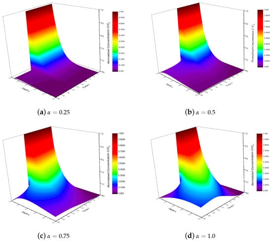
Figure 1.
Concentration distribution of AB-ADM with linear adsorption in Equation (11) with different values when , , , , .
For the limit of time , cases for different concentration sources can be derived.
3.1. AB-ADM with Linear Adsorption for Pulse-like Input Source
When , , it develops into
Through a similar process of calculation, the exact solution to Equation (12) can be represented as
When , Equation (13) is reduced to
Figure 2 indicates that the suggested model in Equation (13) fits the experimental data [45] well and is appropriate to describe advection dispersion problems. The numerical simulations of the AB-ADM in Equation (13) for different values are displayed in Figure 3.
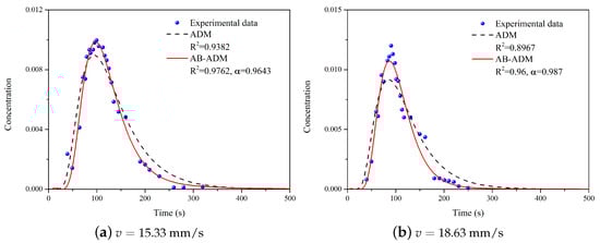
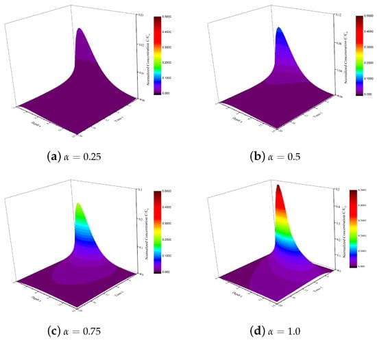
Figure 3.
Concentration distributions of AB-ADM with linear adsorption for an instantaneous concentration source in Equation (13) with different values when , , , .
3.2. AB-ADM with Linear Adsorption for Constant Concentration Source
When , , it comes to
Further, the exact analytic solution of the AB-ADM in Equation (15) is
When , Equation (16) can be presented as
which is the asymmetrical solution to the classical ADM proposed by Ogata and Banks [46].
Figure 4 indicates that the AB-ADM in Equation (16) fits the experimental data better than the classical ADM in Equation (17). The numerical simulations of the AB-ADM in Equation (16) are exhibited in Figure 5.
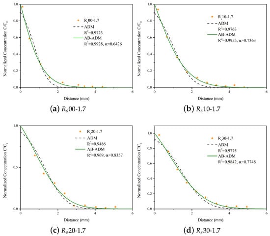
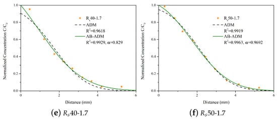
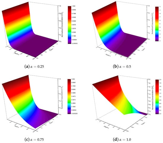
Figure 5.
Numerical simulations of AB-ADM with linear adsorption for a constant concentration source in Equation (16) with different values when , , , .
4. The AB-ADM with First-Order Decay
If it is assumed that the contaminant transport is subject to first-order decay without multi-step or nonlinear reactions, then the sinks or source term is
where is the decay constant.
Integrating Equation (18) into Equation (3) results in
Introducing the new function satisfied , and making use of F.S.T. and L.T. with Equation (19) develops into
where
, ; employing I.F.S.T. and inverse L.T. to Equation (21) results in
where .
Further, when I.F.S.T. and inverse L.T. are employed with Equation (20), considering Equations (A3) and (22), the exact solution of Equation (19) is
where
Figure 6 shows concentration distributions of AB-ADM with first-order decay in Equation (23) for different fractional index values.
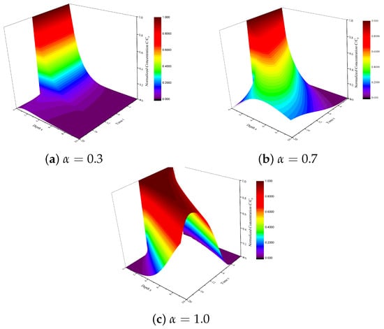
Figure 6.
Numerical simulations of AB-ADM with first-order decay in Equation (23) with different values when , , , , .
It is easy to infer that the hypothesis of a constant source case is valid for a large enough time, . When , it comes to
Similarly, the analytical solution of AB-ADM in Equation (24) is
When ,
the classical symmetric analytical solution of ADM [48] is acquired.
Figure 7 indicates that the fitting results of AB-ADM in Equation (25) with experimental data [49] for long-term tritium transport are better than the fitting results of ADM in Equation (26). The numerical simulations of the AB-ADM in Equation (25) are displayed in Figure 8.
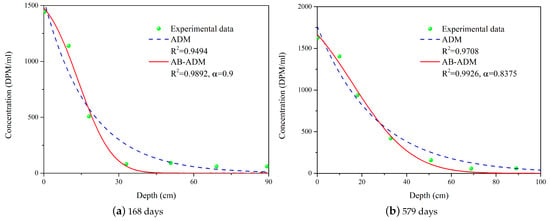
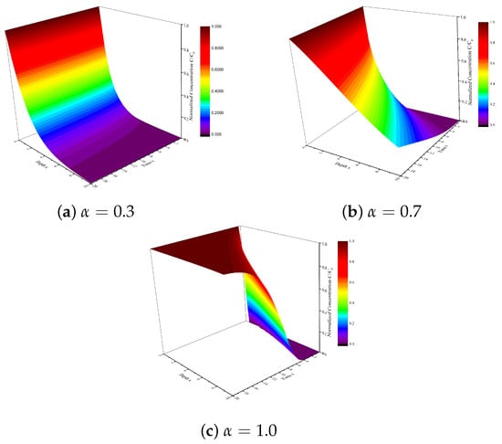
Figure 8.
Numerical simulations of AB-ADM with first-order decay for constant source in Equation (25) with different values when , , and , .
5. Discussion
In this work, the AB differential operator is introduced to the ADM to describe contaminant transport in geological systems. The exact analytic solutions of the new models are given in the light of two cases, including adsorption and first-order decay. The results of the experimental data-fitting analysis indicate that the fractional models provide a relatively more accurate fit. The classical ADMs are demonstrated to be the particular limiting cases of the suggested models. The AB-ADM could be applied to the process of laboratory columns, radionuclide migration, and groundwater solute transport. However, the proposed models still face limitations. Firstly, AB-ADM with linear adsorption neglects nonlinear sorption isotherms (like Freundlich and Langmuir), which are often observed in soils and rocks; this limits applicability. Secondly, the proposed models only considered the first-order decay, which is simplistic, but many contaminants undergo high-order decay or nonlinear reactions, which should also be taken into account. Thirdly, the boundary conditions are somehow idealized for contaminant transport in real geological systems. In addition, the fractional parameter represents the power-law or memory effect in the contaminant transport process, we should further discuss and address its physical meaning. Whether it is linked to pore-scale heterogeneity, memory in adsorption, or anomalous diffusion pathways certainly needs to be validated in further investigations. The AB-ADM with first-order decay is compared with tritium transport data, but long-term predictions and deviations at later times are not analyzed. The benchmarking against other fractional or stochastic models (Caputo-based ADE, continuous-time random walk) is lacking. The presented AB-ADM should help assess and compare different formulations of contaminant transport models in describing anomalous diffusion dynamics. Moreover, different forms of crossovers to normal dynamics should be studied. For practical application in contaminant transport, the most significance is extending AB-ADMs to two- or three-dimensional cases incorporating variable velocity fields, nonlinear sorption, and reactive transport coupling, which would better reflect the natural geological systems. In order to accomplish these generalizations, undertaking an effective (convergent and stable), a numerical simulation is also required. All of these further studies would improve the applicability of AB-ADM and help engineers or hydrogeologists predict contaminant spread more reliably.
6. Conclusions
The AB-ADMs using the AB differential operator are more capable of catching the concentration variation characteristics presented in the real-world experimental data than the traditional ADMs from the data-based fitting results. The AB-ADMs provides flexible and adequate simulations of contaminant transport by selecting different differential-order values. Towards the end, all the results are supported with the assistance of graphical portrayal via a numerical investigation, which would be beneficial for researchers to contemplate the dynamics of the contaminant transport. As a consequence, the proposed AB-ADM provide an effective description of contaminant transport in a geological environment.
Author Contributions
Conceptualization, S.Y. and Q.W.; methodology, Q.W. and S.X.; validation, S.X., Q.W. and L.A.; formal analysis, S.Y.; investigation, L.A.; data curation, Q.W.; writing–original draft preparation, Q.W. and S.Y.; writing–review and editing, S.Y.; visualization, Q.W.; supervision, S.Y. and H.Z.; funding acquisition, S.Y., S.X. and H.Z. All authors have read and agreed to the published version of the manuscript.
Funding
This work was funded by the National Natural Science Foundation of China (52204110, 52574121, 52504102), the Deep Earth Probe and Mineral Resources Exploration-National Science and Technology Major Project (2024ZD1003902), the Intergovernmental International Science and Technology Innovation Cooperation Key Special Project (2025YFE0109800), and the European Commission Horizon Europe Marie Skłodowska-Curie Actions Staff Exchanges Project-LOC3G (101129729).
Data Availability Statement
Data are contained within the article.
Acknowledgments
The authors really appreciate the editors and anonymous reviewers for providing rigorous and constructive suggestions, which have greatly contributed to the improvement of this work.
Conflicts of Interest
The authors declare no conflicts of interest.
Abbreviations
The following abbreviations are used in this manuscript:
| ADM | Advection–dispersion model |
| AB | Atangana–Baleanu |
| AB-ADMs | Atangana–Baleanu advection-dispersion models |
| L.T. | Laplace transform |
| I.L.T. | Inverse Laplace transform |
| F.S.T. | Fourier sine transform |
| I.F.S.T. | Inverse Fourier sine transform |
Appendix A. Integral Transforms
We give the basic mathematical formula used in the calculation process. The Laplace transform (L.T) [43] of is defined as
In addition, we recall some L.T. of basic functions herein that will be used later in this work [31,43]:
The Fourier sine transform (F.S.T.) [50] of is
and the inverse Fourier sine transform (I.F.S.T.) of is . The properties of F.S.T. are as follows,
References
- Berkowitz, B. Characterizing flow and transport in fractured geological media: A review. Adv. Water Resour. 2002, 25, 861–884. [Google Scholar] [CrossRef]
- Zheng, C.M.; Bennett, G. Applied Contaminant Transport Modeling; Wiley: Hoboken, NJ, USA, 2002. [Google Scholar]
- Medved’, I.; Černý, R. Modeling of radionuclide transport in porous media: A review of recent studies. J. Nucl. Mater. 2019, 526, 151765. [Google Scholar] [CrossRef]
- Ajayi, I.R.; Fischer, H.W.; Burak, A.; Qwasmeh, A.; Tabot, B. Concentration and vertical distribution of 137Cs in the undisturbed soil of southwestern Nigeria. Health Phys. 2007, 92, 73. [Google Scholar] [CrossRef]
- Krsti, D.; Nikezi, D.; Stevanovi, N.; Jeli, M. Vertical profile of 137Cs in soil. Appl. Radiat. Isot. 2004, 61, 1487–1492. [Google Scholar] [CrossRef]
- Pang, L.; Goltz, M.; Close, M. Application of the method of temporal moments to interpret solute transport with sorption and degradation. J. Contam. Hydrol. 2003, 60, 123–134. [Google Scholar] [CrossRef]
- Casey, F.; Ong, S.K.; Horton, R. Degradation and transformation of trichloroethylene in miscible-displacement experiments through zerovalent metals. Environ. Sci. Technol. 2000, 34, 5023–5029. [Google Scholar] [CrossRef]
- Chen, T.; Sun, M.; Li, C.; Tian, W.; Liu, X.; Wang, L.; Wang, X.; Liu, C. The influence of temperature on the diffusion of 125I in Beishan granite. Int. J. Chem. Asp. Nucl. Sci. Technol. 2010, 98, 301–305. [Google Scholar] [CrossRef]
- Chen, T.; Li, C.; Liu, X.Y.; Wang, L. Migration study of iodine in Beishan granite by a column method. J. Radioanal. Nucl. Chem. 2013, 298, 219–225. [Google Scholar] [CrossRef]
- Zhang, X.X.; Crawford, J.W.; Deeks, L.K.; Stutter, M.I.; Bengough, A.G.; Young, I.M. A mass balance based numerical method for the fractional advection-dispersion equation: Theory and application. Water Resour. Res. 2005, 41, 62–75. [Google Scholar] [CrossRef]
- Hatano, Y.; Hatano, N. Dispersive transport of ions in column experiments: An explanation of long-tailed profiles. Water Resour. Res. 1998, 34, 1027–1034. [Google Scholar] [CrossRef]
- Raveh-Rubin, S.; Edery, Y.; Dror, I.; Berkowitz, B. Nickel migration and retention dynamics in natural soil columns. Water Resour. Res. 2015, 51, 7702–7722. [Google Scholar] [CrossRef]
- Podlubny, I. Fractional Differential Equations, Mathematics in Science and Engineering; Academic Press: New York, NY, USA, 1999. [Google Scholar]
- Mainardi, F. Fractional Calculus and Waves in Linear Viscoelasticity: An Introduction to Mathematical Models; World Scientific: Singapore, 2010. [Google Scholar]
- Evangelista, L.R.; Lenzi, E.K. Fractional Diffusion Equations and Anomalous Diffusion; Cambridge University Press: Cambridge, UK, 2018. [Google Scholar]
- Chen, K.W.; Zhan, H.B.; Yang, Q. Fractional models simulating non-Fickian behavior in four stage single well push pull tests. Water Resour. Res. 2017, 53, 9528–9545. [Google Scholar] [CrossRef]
- Yang, S.; Song, H.C.; Zhou, H.W.; Xie, S.L.; Zhang, L.; Zhou, W.T. A fractional derivative insight into full-stage creep behavior in deep coal. Fractal Fract. 2025, 9, 473. [Google Scholar] [CrossRef]
- Chen, W.; Sun, H.G.; Li, X. Fractional Derivative Modeling in Mechanics and Engineering; Springer Nature: Berlin/Heidelberg, Germany, 2022. [Google Scholar]
- Yang, S.; Jia, W.H.; Xie, S.L.; Wang, H.C.; An, L. Fractional modeling of deep coal rock creep considering strong time-dependent behavior. Mathematics 2025, 13, 3247. [Google Scholar] [CrossRef]
- Caputo, M. Linear models of dissipation whose Q is almost frequency independent. Ann. Geophys. 1966, 19, 383–393. [Google Scholar] [CrossRef]
- Zhou, H.W.; Yang, S. Fractional derivative approach to non-Darcian flow in porous media. J. Hydrol. 2018, 566, 910–918. [Google Scholar] [CrossRef]
- Benson, D.A.; Meerschaert, M.M.; Revielle, J. Fractional calculus in hydrologic modeling: A numerical perspective. Adv. Water Resour. 2013, 51, 479–497. [Google Scholar] [CrossRef]
- Caputo, M.; Plastino, W. Diffusion in porous layers with memory. Geophys. J. Int. 2004, 158, 385–396. [Google Scholar] [CrossRef]
- Caputo, M. Diffusion of fluids in porous media with memory. Geothermics 1999, 28, 113–130. [Google Scholar] [CrossRef]
- Caputo, M.; Fabrizio, M. A new definition of fractional derivative without singular kernel. Prog. Fract. Differ. Appl. 2015, 1, 73–85. [Google Scholar]
- Sheikh, N.A.; Ali, F.; Khan, I.; Saqib, M. A modern approach of Caputo–Fabrizio time-fractional derivative to MHD free convection flow of generalized second-grade fluid in a porous medium. Neural Comput. Appl. 2018, 30, 1865–1875. [Google Scholar] [CrossRef]
- Wei, Q.; Zhou, H.W.; Yang, S. Non-Darcy flow models in porous media via Atangana-Baleanu derivative. Chaos Solitons Fractals 2020, 141, 110335. [Google Scholar] [CrossRef]
- Khan, M.A.; Hammouch, Z.; Baleanu, D. Modeling the dynamics of hepatitis E via the Caputo–Fabrizio derivative. Math. Model. Nat. Phenom. 2019, 14, 311. [Google Scholar] [CrossRef]
- Baleanu, D.; Mohammadi, H.; Rezapour, S. A fractional differential equation model for the COVID-19 transmission by using the Caputo–Fabrizio derivative. Adv. Differ. Equ. 2020, 2020, 1–27. [Google Scholar] [CrossRef] [PubMed]
- Baleanu, D.; Jajarmi, A.; Mohammadi, H.; Rezapour, S. A new study on the mathematical modelling of human liver with Caputo–Fabrizio fractional derivative. Chaos Solitons Fractals 2020, 134, 109705. [Google Scholar] [CrossRef]
- Atangana, A.; Baleanu, D. New fractional derivatives with nonlocal and non-singular kernel: Theory and application to heat transfer model. Therm. Sci. 2016, 20, 763–769. [Google Scholar] [CrossRef]
- Yu, Y.J.; Deng, Z.C. Fractional order theory of cattaneo-type thermoelasticity using new fractional derivatives. Appl. Math. Model. 2020, 87, 731–751. [Google Scholar] [CrossRef]
- Wei, Q.; Yang, S.; Zhou, H.W.; Zhang, S.Q.; Li, X.N.; Hou, W. Fractional diffusion models for radionuclide anomalous transport in geological repository systems. Chaos Solitons Fractals 2021, 146, 110863. [Google Scholar] [CrossRef]
- Sin, C.S.; Zheng, L.C.; Sin, J.S.; Liu, F.W.; Liu, L. Unsteady flow of viscoelastic fluid with the fractional K-BKZ model between two parallel plates. Appl. Math. Model. 2017, 47, 114–127. [Google Scholar] [CrossRef]
- Kundu, S.; Ghoshal, K. Effects of non-locality on unsteady nonequilibrium sediment transport in turbulent flows: A study using space fractional ADE with fractional divergence. Appl. Math. Model. 2021, 96, 617–644. [Google Scholar] [CrossRef]
- Mirza, I.A.; Akram, M.S.; Shah, N.A.; Imtiaz, W.; Chung, J.D. Analytical solutions to the advection-diffusion equation with Atangana-Baleanu time-fractional derivative and a concentrated loading. Alex. Eng. J. 2021, 60, 1199–1208. [Google Scholar] [CrossRef]
- Berkowitz, B.; Cortis, A.; Dentz, M.; Scher, H. Modeling non-Fickian transport in geological formations as a continuous time random walk. Rev. Geophys. 2006, 44, RG2003. [Google Scholar] [CrossRef]
- Haggerty, R.; Gorelick, S.M. Multiple-rate mass transfer for modeling diffusion and surface reactions in media with pore-scale heterogeneity. Water Resour. Res. 1995, 31, 2383–2400. [Google Scholar] [CrossRef]
- Schumer, R.; Benson, D.A.; Meerschaert, M.M.; Baeumer, B. Fractal mobile/immobile solute transport. Water Resour. Res. 2003, 39, 1296. [Google Scholar] [CrossRef]
- Jury, W.A.; Roth, K. Transfer Functions and Solute Movement Through Soil: Theory and Applications; Birkhauser Verlag: Basel, Switzerland, 1990. [Google Scholar]
- Marino, M.A. Distribution of contaminants in porous media flow. Water Resour. Res. 1974, 10, 1013–1018. [Google Scholar] [CrossRef]
- Bear, J. Dynamics of Fluids in Porous Media; American Elsevier Publication: New York, NY, USA, 1972. [Google Scholar]
- Kilbas, A.A.; Srivastava, H.M.; Trujillo, J.J. Theory and applications of fractional differential equations. In North-Holland Mathematics Studies; Elsevier Science: Amsterdam, The Netherlands, 2006; Volume 204. [Google Scholar]
- Legua, M.P.; Morales, I.; Ruiz, L.M.S. The heaviside step function and matlab. In Computational Science and Its Applications—ICCSA 2008; Springer: Berlin/Heidelberg, Germany, 2008; pp. 1212–1221. [Google Scholar]
- Qian, J.Z.; Chen, Z.; Zhan, H.B.; Luo, S.H. Solute transport in a filled single fracture under non-darcian flow. Int. J. Rock Mech. & Min. Sci. 2011, 48, 132–140. [Google Scholar] [CrossRef]
- Ogata, A.; Banks, R. A Solution of the Differential Equation of Longitudinal Dispersion in Porous Media; Geological Survey Professional Paper 411 (A); U.S. Geological Survey: Reston, VA, USA, 1961. [Google Scholar] [CrossRef]
- Lang, Z.; Zhang, H.; Ming, Y.; Hang, C.; Ming, Z. Laboratory determination of migration of Eu(III) in compacted bentonite-sand mixtures as buffer/backfill material for high-level waste disposal. Appl. Radiat. Isot. 2013, 82, 139–144. [Google Scholar] [CrossRef]
- Genuchten, M.T.V.; Alves, W.J. Analytical Solutions of the One-Dimensional Convective-Dispersive Solute Transport Equation; Technical Bulletin No. 1661; US Department of Agriculture, Agricultural Research Service: Beltsville, MA, USA, 1982. [CrossRef]
- Toupiol, C.; Willingham, T.W.; Valocchi, A.J.; Werth, C.J.; Krapac, I.G.; Stark, T.D.; Daniel, D.E. Long-term tritium transport through field-scale compacted soil liner. J. Geotech. Geoenviron. Eng. 2002, 128, 640–650. [Google Scholar] [CrossRef][Green Version]
- Debnath, L.; Bhatta, D. Integral Transforms and Their Applications, 3rd ed.; Taylor & Francis Group: Abingdon, UK, 2015. [Google Scholar]


Disclaimer/Publisher’s Note: The statements, opinions and data contained in all publications are solely those of the individual author(s) and contributor(s) and not of MDPI and/or the editor(s). MDPI and/or the editor(s) disclaim responsibility for any injury to people or property resulting from any ideas, methods, instructions or products referred to in the content. |
© 2025 by the authors. Licensee MDPI, Basel, Switzerland. This article is an open access article distributed under the terms and conditions of the Creative Commons Attribution (CC BY) license (https://creativecommons.org/licenses/by/4.0/).