Article

Mathematical Perspectives of a Coupled System of Nonlinear Hybrid Stochastic Fractional Differential Equations

1
Department of Mathematics, College of Science, University of Ha’il, Ha’il 55473, Saudi Arabia
2
Department of Mathematics and Statistics, Imam Mohammad Ibn Saud Islamic University (IMSIU), Riyadh 13318, Saudi Arabia
3
Department of Mathematics and Statistics, University of Swat, Swat 19200, Pakistan
4
Department of Mathematics, Faculty of Science, Islamic University of Madinah, Madinah 42351, Saudi Arabia
5
Department of Mathematics, College of Science, Qassim University, Buraydah 51452, Saudi Arabia
*
Authors to whom correspondence should be addressed.
Fractal Fract. 2025, 9(10), 622; https://doi.org/10.3390/fractalfract9100622
Submission received: 17 August 2025 / Revised: 8 September 2025 / Accepted: 15 September 2025 / Published: 24 September 2025

Abstract

This research develops a novel coupled system of nonlinear hybrid stochastic fractional differential equations that integrates neutral effects, stochastic perturbations, and hybrid switching mechanisms. The system is formulated using the Atangana–Baleanu–Caputo fractional operator with a non-singular Mittag–Leffler kernel, which enables accurate representation of memory effects without singularities. Unlike existing approaches, which are limited to either neutral or hybrid stochastic structures, the proposed framework unifies both features within a fractional setting, capturing the joint influence of randomness, history, and abrupt transitions in real-world processes. We establish the existence and uniqueness of mild solutions via the Picard approximation method under generalized Carathéodory-type conditions, allowing for non-Lipschitz nonlinearities. In addition, mean-square Mittag–Leffler stability is analyzed to characterize the boundedness and decay properties of solutions under stochastic fluctuations. Several illustrative examples are provided to validate the theoretical findings and demonstrate their applicability.

1. Introduction

This study focuses on the qualitative analysis of a coupled system of fractional hybrid neutral stochastic differential equations. In this section, we presented some fundamentals of fractional calculus (FC), coupled systems, hybrid differential equations, and literature concerning these significant aspects of FC.

1.1. Fractional Calculus

In the modern era, FC plays a vital role due to its potential applications in epidemic modeling, viscoelastic material control, population growth, and smart engineering systems. FC is the study of non-integer order derivatives and integrals, evolving from purely theoretical aspects into a powerful tool for modeling real-world phenomena characterized by memory, nonlocality, and hereditary effects [1,2,3,4]. Classical differential equations (DEs) often fall short when describing materials or processes where the present state depends not only on the current conditions but also on historical behavior. These significant aspects of FC have led to the development of various fractional derivatives (FDs), including the Riemann–Liouville, Hosmanard, Grünwald–Letnikov, Caputo, and, more recently, the Atangana–Baleanu (AB) derivatives [5]. Among the different types of FDs, each has its own advantages and limitations under certain circumstances. One of the most important classes is the Atangana–Baleanu–Caputo (ABC) derivative, defined with a non-singular Mittag-Leffler kernel, which has received significant attention due to its ability to preserve memory without introducing singularities [6]. The advantages of the ABC derivative allow for better investigation of stability analysis and physical interpretation, especially in modeling viscoelastic materials, anomalous diffusion, biological systems, and control processes [7].
An important aspect of FC is the study of fractional differential equations (FDEs) from different points of view, such as theoretical insight and numerical approximations. Researchers employ FDEs for accurate and reliable modeling of dynamical systems involving sudden fluctuations, long-term memory, and non-local effects. One notable class of these DEs is stochastic differential equations (SDEs). SDEs introduce random perturbations into dynamical systems, often represented through Wiener processes or white noise [8]. They are essential for understanding systems affected by uncertainty, noise, or incomplete information, such as financial models (e.g., the Black–Scholes equation), control systems, and gene expression under stochastic regulation in noisy environments. SDEs have become a fundamental framework in fields such as statistical physics, quantitative finance, epidemiology, and machine learning [9,10,11,12]. Moreover, SDEs allow analysis not only of mean trajectories but also of variances and probabilistic bounds.

1.2. Coupled System and Hybrid Differential Equations

A system of multi-differential equations containing interdependent variables and their derivatives, where the evolution of each dependent variable depends on the others, is called a coupled system of differential equations (CSDE). In certain circumstances, real-world problems arise in the form of CSDEs. Such systems describe multiple interacting subsystems that evolve together through interdependence. They can capture a wide range of phenomena, including cooperative dynamics, synchronized behaviors, and feedback regulation. Common examples of CSDEs include multi-agent robotics, reaction–diffusion systems in chemistry, electrical oscillator networks, and interconnected ecological models such as predator–prey dynamics [13,14]. This type of coupling structure allows for rich dynamical behavior, such as phase locking or multi-stability, that cannot be modeled by isolated systems. These systems play a crucial role in both the modeling and control of distributed systems. Recently, a class of CSDEs, i.e., coupled systems of hybrid neutral stochastic fractional differential equations (HNSFDEs), has gained more attention from researchers around the globe. HNSFDEs represent systems that exhibit both continuous evolution and discrete transitions [15]. Neutral differential equations (NDEs) extend the concepts of delay differential equations (DDEs) by incorporating dependence on past derivatives, making them particularly useful for modeling systems with memory-dependent dynamics, such as circuit networks or viscoelastic materials with transmission delays [16]. These models are essential for accurately describing processes where abrupt changes, switching dynamics, or threshold-based decisions coexist with smooth temporal evolution. Hybrid systems naturally arise in power electronics (e.g., switching converters), robotics (e.g., legged locomotion), biochemical networks (e.g., gene regulation), and cyber–physical systems where digital logic interacts with analog physical processes [17,18]. By blending discrete and continuous behaviors, hybrid models offer a more flexible and realistic description of systems with regime-switching dynamics and logic-driven feedback.
Hybrid differential equations combined with neutral stochastic differential equations (NSDEs) model complex systems where continuous random fluctuations interact with sudden discrete transitions [19]. When hybrid behavior and stochastic effects are embedded within a fractional framework, we obtain a powerful unified tool for modeling complex phenomena in neural networks, fractional order sliding mode control multiagent system with time-varying delays [20], epidemic propagation [21], and industrial automation [22], finite time stability results were deduced for fractional-order hydraulic turbine regulating system [23], regime switching [24], and Mittag-Leffler stability for Hopfield neural networks [25]. These systems appear in financial markets experiencing both Brownian-motion-driven price changes and abrupt regime shifts and in biological systems where stochastic chemical reactions coexist with discrete cellular events [26]. This mathematical framework typically involves an SDE governing the continuous state dynamics, coupled with a Markov chain or deterministic switching mechanism that triggers instantaneous jumps in system parameters [27]. Such models require specialized analytical techniques, including extended versions of Itô’s calculus and piecewise deterministic Markov process theory. The applications of coupled systems of HNSDEs range from robotics to power systems, where purely continuous or purely discrete models prove inadequate. The study draws on tools from stochastic analysis, dynamical systems theory, and control engineering to address these hybrid stochastic dynamics [28]. Likewise, HNSDEs are effective tools for modeling smart energy grids, where the neutral nature is used for voltage regulation, stochasticity arises from renewable energy output, and switching between power sources ensures stability despite unsteady supply and demand [29]. HNSDEs also play a vital role in biomedical systems, optimizing drug delivery by addressing delayed metabolic reactions, adaptive dosage adjustments, and random patient responses, leading to more effective and precise treatments [30]. To handle such significant and complex problems, specialized techniques are required, whether analyzing almost-sure stability in stochastic cases or developing adaptive solvers for their deterministic counterparts [31].

1.3. Related Literature to the Study

The existence and uniqueness (EU) of solutions to SDEs driven by Brownian motion are widely examined in the literature [32]. Additionally, significant attention has been given to extending the qualitative theory of SDEs to infinite-dimensional settings [33,34]. Among these developments, Taniguchi [35] demonstrates EU results for SDEs under generalized non-Lipschitz conditions on the drift and diffusion terms, which encompass earlier findings of Yamada as a special case. Further contributions by Yamada [36], Rodkina [37], and Taniguchi [35] provided analogous EU theorems for ordinary SDEs with non-Lipschitz coefficients. In addition, Vinayagam and Balasubramaniam [38] explored the existence of mild solutions (MSs) for a specific category of non-linear neutral SDEs formulated in Hilbert spaces. Meanwhile, Jiang and Shen [39] advanced the theory by analyzing EU for neutral stochastic partial functional DEs under certain Carathéodory-type coefficient conditions. Their approach relied on successive approximation methods and led to generalizations of earlier work, including results from [40]. Arzu and Nazim [41] extended the EU of MSs to general fractional neutral SDEs under Carathéodory-type conditions (CTCs) on the coefficients using the well-known Picard iterative method (PIM).

1.4. New Findings

After reviewing the existing literature on the existence theory of FSDEs and considering the aforementioned research, this study uses the PIM to generalize the results concerning EU of mild solutions and mean square stability analysis for the proposed novel coupled system of HNSFDEs (1) under CTC on the coefficients. The proposed generalized coupled system of HNSFDEs with ( ν ( 1 2 , 1 ) ) is given by
D 0 + ν ABC ( Ψ ( t ) + g 1 ( t , Ψ ( t ) ) ) = A 1 Ψ ( t ) + F 1 ( t , Υ ( t ) ) + σ 1 ( t , Ψ ( t ) ) d W ( t ) d t , D 0 + ν ABC ( Υ ( t ) + g 2 ( t , Υ ( t ) ) ) = A 2 Υ ( t ) + F 2 ( t , Ψ ( t ) ) + σ 2 ( t , Υ ( t ) ) d W ( t ) d t , Ψ ( 0 ) = α 1 , Υ ( 0 ) = α 2 ,
where D 0 + ν ABC is the ABC fractional derivative, ( W ( t ) ) t 0 is a standard Brownian motion on a complete probability space ( Ω , F T , P ) for T 0 , with some filtration F T : = { F t } t [ 0 , t ] satisfying the usual conditions (i.e., F 0 consists of all P -null sets, while it is right-continuous and increasing), where g 1 ,   g 2 : [ 0 , t ] × R d R d are the nonlinear functions defining the neutral terms. The functions F 1 ,   F 2 represent the nonlinear drift terms, and σ 1 ,   σ 2 are the diffusion coefficients governing the stochastic perturbations. The initial conditions α 1 ,   α 2 are F 0 -measurable H-valued random variables, and A 1 , A 2 R d × d .
Previous studies on neutral FSDEs have mainly focused on simple forms using classical derivatives, and primarily from the existence perspective. This work addresses the following novel aspects, which were not yet been analyzed to the best of our knowledge, particularly in terms of stability:
  • We introduce the idea of coupling neutral DEs with hybrid stochasticity, thereby advancing research in new directions by formulating a more realistic and mathematically enriched model.
  • By incorporating hybrid differential structures, our model accounts for both continuous dynamics and discrete regime-switching behavior.
  • Instead of relying on traditional fractional derivatives, which involve singular kernels and associated limitations, we employ the ABC derivative with a non-singular Mittag-Leffler kernel.
  • We establish the mean-square Mittag-Leffler stability of the proposed system, ensuring that solutions remain bounded and decay predictably under stochastic fluctuations.
  • To the best of our knowledge, mean-square stability analysis for both simple and coupled systems of FSDEs has not yet been investigated.
We address the theoretical gap by formulating a nonlinear coupled system of hybrid stochastic differential equations using the ABC derivative, establishing existence and uniqueness under CTC via the Picard approximation and proving mean-square Mittag-Leffler stability for reliable applications in engineering, neuroscience, epidemiology, and control systems. The introduction of these aspects into existing models enhances theoretical and mathematical understanding. In particular, by extending a single SDE to a coupled system of FSDEs with hybrid concepts, which allow for mutual interactions between subsystems, an essential feature in modeling real-world phenomena such as interconnected biological systems and cyber–physical infrastructures. The stability property reinforces the robustness and applicability of our framework, making it a powerful generalization of existing models and highly suitable for simulating complex, real-world dynamical systems, which have not yet been studied. The investigation of the proposed coupled system of HNSDEs also provides new directions for researchers to establish further results regarding the existence of mild solutions and stability analysis.

2. Preliminaries

We present essential structures of fractional calculus and necessary facts about fractional stochastic neutral differential systems.
Definition 1 
([5]). For a function f A C ( [ a , b ] ) and 0 < ν < 1 , the ABC fractional derivative is defined as
D a ν ABC f ( t ) = C ( ν ) 1 ν a t f ( δ ) E ν ν ( t δ ) ν ν 1 d δ .
Definition 2
([42]). The associated ABC fractional integral is given by
I a ν ABC f ( t ) = 1 ν C ( ν ) f ( t ) + ν C ( ν ) Γ ( ν ) a t ( t δ ) ν 1 f ( δ ) d δ .
where Γ ( · ) is the Gamma function:
Γ ( ν ) : = 0 δ ν 1 e δ d δ ,
and C ( ν ) is a normalization function with C ( 0 ) = C ( 1 ) = 1 , and E ν ( · ) is the Mittag-Leffler function (MLF).
Definition 3 
([43]). MLF, in two parameters,
E ν , β ( z ) = k = 0 z k Γ ( k u + β ) , ν , β > 0 ,
with its matrix version,
E ν , β ( t ν A ) = k = 0 A k t k u Γ ( k u + β ) , A R n × n ,
satisfying:
D 0 + ν C E ν ( t ν A ) = A E ν ( t ν A ) .
Definition 4 
([44]). Let ( Ψ ( t ) , Υ ( t ) ) be a mild solution of the coupled system on [ 0 , t ] . The system is said to be mean-square Mittag-Leffler-stable, if there exist constants C > 0 , λ > 0 , and 0 < ν < 1 such that
E Υ ( t ) 2 + E Ψ ( t ) 2 C E ν ( λ t ν ) ( E α 1 2 + E α 2 2 ) .
Let R d be endowed with the standard Euclidean norm, and let H 2 ( [ 0 , t ] , R d ) denote the space of all F T -measurable processes ξ satisfying:
H 2 ( [ 0 , t ] , R d ) : = ξ : ξ H 2 2 = sup t [ 0 , t ] E ξ ( t ) 2 < .
Lemma 1. 
Assume that Ψ ( δ ) is an H-valued process which satisfies E 0 T Ψ ( δ ) 2 d δ < . Then, for every 0 < T and 2 ν > 1 , there exists a constant C T = T 2 ν 1 2 ν 1 such that
sup 0 t T E 0 t ( t δ ) ν 1 Ψ ( δ ) d W ( δ ) 2 C T E 0 T Ψ ( δ ) 2 d δ .
Apparently, (8) is a Banach space, and g i ,   F i ,   σ i : [ 0 , t ] × R d R d are bounded and measurable functions that satisfy the following assumptions:
Assumption 1.
( A 1 ) :
The functions g i satisfy E g i ( t , Ψ ) g i ( t , Y ) 2 L i 2 E Ψ Y 2 with 0 < L i < 1 2 .
( A 2 ) :
The drift and diffusion terms satisfy
F 1 ( t , Ψ 1 , Υ 1 ) F 1 ( t , Ψ 2 , Υ 2 ) 2   L F 1 ( Ψ 1 Ψ 2 2 +   Υ 1 Υ 2 2 ) , σ 1 ( t , Ψ ) σ 1 ( t , Υ ) 2   L σ 1 Ψ Υ 2 , F 2 ( t , Ψ 1 , Υ 1 ) F 2 ( t , Ψ 2 , Υ 2 ) 2   L F 2 ( Ψ 1 Ψ 2 2 +   Υ 1 Υ 2 2 ) , σ 2 ( t , Υ 1 ) σ 2 ( t , Υ 2 ) 2   L σ 2 Υ 1 Υ 2 2 .
( A 3 ) :
Linear growth conditions hold: F i ( t , 0 , 0 ) 2 + σ i ( t , 0 ) 2 K i < .

3. Results of Existence

Lemma 2. 
The mild solution to the coupled system of NHSFDEs (1) with order ν ( 0.5 , 1 ) , is given by
Ψ ( t ) = α 1 + g 1 ( 0 , α 1 ) g 1 ( t , Ψ ( t ) ) + 1 ν C ( ν ) F 1 ( t , Υ ( t ) ) + A 1 Ψ ( t ) + ν C ( ν ) Γ ( ν ) 0 t ( t δ ) ν 1 F 1 ( δ , Υ ( δ ) ) + A 1 Ψ ( δ ) d δ + 1 ν C ( ν ) σ 1 ( t , Ψ ( t ) ) W ˙ ( t ) + ν C ( ν ) Γ ( ν ) 0 t ( t δ ) ν 1 σ 1 ( δ , Ψ ( δ ) ) d W ( δ ) ,
Υ ( t ) = α 2 + g 2 ( 0 , α 2 ) g 2 ( t , Υ ( t ) ) + 1 ν C ( ν ) F 2 ( t , Ψ ( t ) ) + A 2 Υ ( t ) + ν C ( ν ) Γ ( ν ) 0 t ( t δ ) ν 1 F 2 ( δ , Ψ ( δ ) ) + A 2 Υ ( t ) d δ + 1 ν C ( ν ) σ 2 ( t , Υ ( t ) ) W ˙ ( t ) + ν C ( ν ) Γ ( ν ) 0 t ( t δ ) ν 1 σ 2 ( δ , Υ ( δ ) ) d W ( δ ) .
Proof. 
We consider the coupled system of NHSFDEs (1) involving the ABC fractional derivative with ν ( 1 2 , 1 ) . Applying I 0 ν ABC on both sides of the system and using the identity
I 0 ν ABC D 0 ν ABC f ( t ) = f ( t ) f ( 0 ) ,
we obtain
Ψ ( t ) + g 1 ( t , Ψ ( t ) ) = α 1 + g 1 ( 0 , α 1 ) + I 0 ν ABC A 1 Ψ ( t ) + F 1 ( t , Υ ( t ) ) + σ 1 ( t , Ψ ( t ) ) d W ( t ) d t , Υ ( t ) + g 2 ( t , Υ ( t ) ) = α 2 + g 2 ( 0 , α 2 ) + I 0 ν ABC A 2 Υ ( t ) + F 2 ( t , Ψ ( t ) ) + σ 2 ( t , Υ ( t ) ) d W ( t ) d t .
Subtracting the nonlinear terms g 1 ( t , Ψ ( t ) ) and g 2 ( t , Υ ( t ) ) , we have
Ψ ( t ) = α 1 + g 1 ( 0 , α 1 ) g 1 ( t , Ψ ( t ) ) + I 0 ν ABC A 1 Ψ ( t ) + F 1 ( t , Υ ( t ) ) + σ 1 ( t , Ψ ( t ) ) d W ( t ) d t , Υ ( t ) = α 2 + g 2 ( 0 , α 2 ) g 2 ( t , Υ ( t ) ) + I 0 ν ABC A 2 Υ ( t ) + F 2 ( t , Ψ ( t ) ) + σ 2 ( t , Υ ( t ) ) d W ( t ) d t .
Applying the ABC Integral to each term,
  • For I 0 + ν ABC [ A 1 Ψ ( t ) ]
    I 0 + ν ABC [ A 1 Ψ ( t ) ] = 1 ν C ( ν ) A 1 Ψ ( t ) + ν C ( ν ) Γ ( ν ) 0 t ( t δ ) ν 1 A 1 Ψ ( δ ) d δ .
  • For I 0 + ν ABC [ F 1 ( t , Υ ( t ) ) ] :
    I 0 + ν ABC [ F 1 ( t , Υ ( t ) ) ] = ν C ( ν ) Γ ( ν ) 0 t ( t δ ) ν 1 F 1 ( δ , Υ ( δ ) ) d δ + 1 ν C ( ν ) F 1 ( t , Υ ( t ) ) .
  • For the stochastic term,
    I 0 + ν ABC [ σ 1 ( t , Ψ ( t ) ) d W ( t ) d t ] ν C ( ν ) Γ ( ν ) 0 t ( t δ ) ν 1 σ 1 ( δ , Ψ ( δ ) ) d W ( δ ) .
  • We use the term ν C ( ν ) Γ ( ν ) 0 t ( t s ) ν 1 σ 1 ( δ , Ψ ( δ ) ) d W ( δ ) from (12) instead of I 0 + ν ABC [ σ 1 ( t , Ψ ( t ) ) d W ( t ) d t ] in the Itô calculus for simplicity.
  • Putting these in the original equation, we get
Ψ ( t ) = α 1 + g 1 ( 0 , α 1 ) g 1 ( t , Ψ ( t ) ) + 1 ν C ( ν ) F 1 ( t , Υ ( t ) ) + A 1 Ψ ( t ) + ν C ( ν ) Γ ( ν ) 0 t ( t δ ) ν 1 F 1 ( δ , Υ ( δ ) ) + A 1 Ψ ( t ) d δ + 1 ν C ( ν ) σ 1 ( t , Ψ ( t ) ) W ˙ ( t ) + ν C ( ν ) Γ ( ν ) 0 t ( t δ ) ν 1 σ 1 ( δ , Ψ ( δ ) ) d W ( δ ) .
A similar procedure follows for the mild solution of Υ ( t ) ,
Υ ( t ) = α 2 + g 2 ( 0 , α 2 ) g 2 ( t , Υ ( t ) ) + 1 ν C ( ν ) A 2 Υ ( t ) + F 2 ( t , Ψ ( t ) ) + ν C ( ν ) Γ ( ν ) 0 t ( t δ ) ν 1 A 2 Υ ( δ ) + F 2 ( δ , Ψ ( δ ) ) d δ + 1 ν C ( ν ) σ 2 ( t , Υ ( t ) ) W ˙ ( t ) + ν C ( ν ) Γ ( ν ) 0 t ( t δ ) ν 1 σ 2 ( δ , Υ ( δ ) ) d W ( δ ) .
These represent the required mild solutions. □

3.1. Results with Lipschitz Coefficients

Here, we analyze the ES of solutions to a coupled system of NHSFDEs. The primary focus is on applying a weighted maximum norm to demonstrate that the integral Equation (10) coincides with the mild solution (15).
Theorem 1. 
Under the conditions ( A 1 ) to ( A 3 ), there exists a mild solution ( Ψ ( t ) w h i c h i s u n i q u e , Υ ( t ) ) to the coupled system of NHSFDEs (1), satisfying Ψ ( 0 ) = α 1 , Υ ( 0 ) = α 2 , which can be written in the following way:
Ψ ( t ) = E ν C ( ν ) 1 ν A 1 t ν [ α 1 + g 1 ( 0 , α 1 ) ] g 1 ( t , Ψ ( t ) ) + ν C ( ν ) Γ ( ν ) 0 t ( t δ ) ν 1 F 1 ( δ , Υ ( δ ) ) E ν , ν C ( ν ) 1 ν A 1 ( t δ ) ν d δ + 1 ν C ( ν ) 0 t E ν C ( ν ) 1 ν A 1 ( t δ ) ν σ 1 ( δ , Ψ ( δ ) ) d W ( δ ) + ν C ( ν ) Γ ( ν ) 0 t ( t δ ) ν 1 E ν , ν C ( ν ) 1 ν A 1 ( t δ ) ν σ 1 ( δ , Ψ ( δ ) ) d W ( δ ) ,
and
Υ ( t ) = E ν C ( ν ) 1 ν A 2 t ν [ α 2 + g 2 ( 0 , α 2 ) ] g 2 ( t , Υ ( t ) ) + ν C ( ν ) Γ ( ν ) 0 t ( t δ ) ν 1 E ν , ν C ( ν ) 1 ν A 2 ( t δ ) ν F 2 ( δ , Ψ ( δ ) ) d δ + 1 ν C ( ν ) 0 t E ν C ( ν ) 1 ν A 2 ( t δ ) ν σ 2 ( δ , Υ ( δ ) ) d W ( δ ) + ν C ( ν ) Γ ( ν ) 0 t ( t δ ) ν 1 E ν , ν C ( ν ) 1 ν A 2 ( t δ ) ν σ 2 ( δ , Υ ( δ ) ) d W ( δ ) .
Proof: 
We establish the result using Banach’s fixed point theorem on the product space as the extension of b-matric space defined in [45],
H : = H α 2 ( [ 0 , t ] , R d ) × H α 2 ( [ 0 , t ] , R d ) ,
equipped with the weighted norm:
( Ψ , Υ ) β 2 : = sup t [ 0 , t ] E Ψ ( t ) 2 + E Υ ( t ) 2 E ν 2 ν 1 ( β t 2 ν 1 ) .
Define T = ( T 1 , T 2 ) : H H where
T 1 ( Ψ , Υ ) ( t ) = E ν C ( ν ) 1 ν A 1 t ν [ α 1 + g 1 ( 0 , α 1 ) ] g 1 ( t , Ψ ( t ) ) + ν C ( ν ) Γ ( ν ) 0 t ( t δ ) ν 1 E ν , ν C ( ν ) 1 ν A 1 ( t δ ) ν F 1 ( δ , Υ ( δ ) ) d δ + 1 ν C ( ν ) 0 t E ν C ( ν ) 1 ν A 1 ( t δ ) ν σ 1 ( δ , Ψ ( δ ) ) d W ( δ ) + ν C ( ν ) Γ ( ν ) 0 t ( t δ ) ν 1 E ν , ν C ( ν ) 1 ν A 1 ( t δ ) ν σ 1 ( δ , Ψ ( δ ) ) d W ( δ ) ,
and
T 2 ( Ψ , Υ ) ( t ) = E ν C ( ν ) 1 ν A 2 t ν [ α 2 + g 2 ( 0 , α 2 ) ] g 2 ( t , Υ ( t ) ) + ν C ( ν ) Γ ( ν ) 0 t ( t δ ) ν 1 E ν , ν C ( ν ) 1 ν A 2 ( t δ ) ν F 2 ( δ , Ψ ( δ ) ) d δ + 1 ν C ( ν ) 0 t E ν C ( ν ) 1 ν A 2 ( t δ ) ν σ 2 ( δ , Υ ( δ ) ) d W ( δ ) + ν C ( ν ) Γ ( ν ) 0 t ( t δ ) ν 1 E ν , ν C ( ν ) 1 ν A 2 ( t δ ) ν σ 2 ( δ , Υ ( δ ) ) d W ( δ ) .
For T 1 : Using assumptions ( A 1 ) ( A 3 ) and Hölder’s inequality,
E T 1 ( Ψ 1 , Υ 1 ) ( t ) T 1 ( Ψ 2 , Υ 2 ) ( t ) 2 4 L 1 2 E Ψ 1 ( t ) Ψ 2 ( t ) 2 + 4 M 1 2 A 1 2 T 2 ν 1 2 ν 1 L 1 2 0 t ( t δ ) 2 ν 2 E Ψ 1 ( δ ) Ψ 2 ( δ ) 2 d δ + 4 M 1 2 T 2 ν 1 2 ν 1 L F 1 0 t ( t δ ) 2 ν 2 ( E Ψ 1 ( δ ) Ψ 2 ( δ ) 2 + E Υ 1 ( δ ) Υ 2 ( δ ) 2 ) d δ + 4 M 1 2 L σ 1 0 t ( t δ ) 2 ν 2 E Ψ 1 ( δ ) Ψ 2 ( δ ) 2 d δ , E T 1 ( Ψ 1 , Υ 1 ) ( t ) T 1 ( Ψ 2 , Υ 2 ) ( t ) 2 4 L 1 2 E Ψ 1 ( t ) Ψ 2 ( t ) 2 + 4 u 2 M 1 2 A 1 2 L 1 2 C ( ν ) 2 Γ ( ν ) 2 ( 2 ν 1 ) 0 t ( t δ ) 2 ν 2 E Ψ 1 ( δ ) Ψ 2 ( δ ) 2 d δ + 4 u 2 M 1 2 L F 1 T 2 ν 1 C ( ν ) 2 Γ ( ν ) 2 ( 2 ν 1 ) 0 t ( t δ ) 2 ν 2 ( E Ψ 1 ( δ ) Ψ 2 ( δ ) 2 + E Υ 1 ( δ ) Υ 2 ( δ ) 2 ) d δ + 8 ( 1 ν ) 2 M 1 2 L σ 1 C ( ν ) 2 E Ψ 1 ( t ) Ψ 2 ( t ) 2 + 8 u 2 M 1 2 L σ 1 C ( ν ) 2 Γ ( ν ) 2 ( 2 ν 1 ) 0 t ( t δ ) 2 ν 2 E Ψ 1 ( δ ) Ψ 2 ( δ ) 2 d δ .
For T 2 ,
E T 2 ( Ψ 1 , Υ 1 ) ( t ) T 2 ( Ψ 2 , Υ 2 ) ( t ) 2 4 L 2 2 E Υ 1 ( t ) Υ 2 ( t ) 2 + 4 M 2 2 A 2 2 T 2 ν 1 2 ν 1 L 2 2 0 t ( t δ ) 2 ν 2 E Υ 1 ( δ ) Υ 2 ( δ ) 2 d δ + 4 M 2 2 T 2 ν 1 2 ν 1 L F 2 0 t ( t δ ) 2 ν 2 ( E Ψ 1 ( δ ) Ψ 2 ( δ ) 2 + E Υ 1 ( δ ) Υ 2 ( δ ) 2 ) d δ + 4 M 2 2 L σ 2 0 t ( t δ ) 2 ν 2 E Υ 1 ( δ ) Υ 2 ( δ ) 2 d δ , 4 L 2 2 E Υ 1 ( t ) Υ 2 ( t ) 2 + 4 u 2 M 2 2 A 2 2 L 2 2 C ( ν ) 2 Γ ( ν ) 2 ( 2 ν 1 ) 0 t ( t δ ) 2 ν 2 E Υ 1 ( δ ) Υ 2 ( δ ) 2 d δ + 4 u 2 M 2 2 L F 2 T 2 ν 1 C ( ν ) 2 Γ ( ν ) 2 ( 2 ν 1 ) 0 t ( t δ ) 2 ν 2 ( E Ψ 1 ( δ ) Ψ 2 ( δ ) 2 + E Υ 1 ( δ ) Υ 2 ( δ ) 2 ) d δ + 8 ( 1 ν ) 2 M 2 2 L σ 2 C ( ν ) 2 E Υ 1 ( t ) Υ 2 ( t ) 2 + 8 u 2 M 2 2 L σ 2 C ( ν ) 2 Γ ( ν ) 2 ( 2 ν 1 ) 0 t ( t δ ) 2 ν 2 E Υ 1 ( δ ) Υ 2 ( δ ) 2 d δ .
Dividing both estimates by E 2 ν 1 ( β t 2 ν 1 ) and combining
T ( Ψ 1 , Υ 1 ) T ( Ψ 2 , Υ 2 ) β 2 max 4 L 1 2 + 8 ( 1 ν ) 2 M 1 2 L σ 1 / C ( ν ) 2 1 4 L 1 2 , 4 L 2 2 + 8 ( 1 ν ) 2 M 2 2 L σ 2 / C ( ν ) 2 1 4 L 2 2 + C β ( Ψ 1 , Υ 1 ) ( Ψ 2 , Υ 2 ) β 2 ,
which implies that
T ( Ψ 1 , Υ 1 ) T ( Ψ 2 , Υ 2 ) β 2 ρ ( Ψ 1 , Υ 1 ) ( Ψ 2 , Υ 2 ) β 2 ,
where C collects all the constants from the estimates. Choose a β that is sufficiently large such that
ρ : = 4 max ( L 1 2 , L 2 2 ) 1 4 max ( L 1 2 , L 2 2 ) + C β < 1 ,
This is possible since 0 < L i < 1 2 by assumption ( A 1 ) . Thus, T is a contraction on ( H , · β , R d ) . Hence, by the contraction principle, T has a unique fixed point. □
Further, we require the following results in our work. Using the representation theorem for martingales, i.e., for any function h L 2 ( Ω , F T , R d ) , there exist unique adapted processes θ 1 , θ 2 H α 2 ( [ 0 , t ] , R d ) such that
h = E h + 0 T θ 1 ( δ ) d W ( δ ) + 0 T θ 2 ( δ ) d W ( δ ) .
It is clear that
h = n = 1 d h n e n = n = 1 d E h n + 0 T θ 1 , n ( δ ) d W ( δ ) + 0 T θ 2 , n ( δ ) d W ( δ ) e n ,
where
h n = E h n + 0 T θ 1 , n ( δ ) d W ( δ ) + 0 T θ 2 , n ( δ ) d W ( δ ) ,
h n L 2 ( Ω , F T , R d )
To show uniqueness for the coupled system of NHSFDEs (1), it is important to prove that
Υ ( t , α ) = Ψ ( t , α ) .
For any h L 2 ( Ω , F T , R d ) , we must verify
E Ψ ( t , α ) , h = E Υ ( t , α ) , h .
Equivalently,
E Ψ ( t , α ) Υ ( t , α ) , h = n = 1 d E ( Ψ n ( t , α ) Υ n ( t , α ) ) h n , e n .
Since R d has the Euclidean norm,
E Ψ ( t , α ) Υ ( t , α ) , h 2 n = 1 d E Ψ n ( t , α ) Υ n ( t , α ) h n 2 , d n = 1 d E Ψ n ( t , α ) Υ n ( t , α ) h n 2 .
Before finding E Ψ ( t , n ) Υ ( t , n ) , h . Define the following measurable and bounded functions:
Ψ n ( t ) = E Ψ n ( t , α ) h n , ν n ( t ) = E ϝ 1 , n ( t , Υ ( t , α ) ) h n , ω n ( t ) = E g 1 , n ( t , Ψ ( t , α ) ) h n , Ψ ˜ n ( t ) = E Υ n ( t , α ) h n , ν ˜ n ( t ) = E F 2 , n ( t , Ψ ( t , α ) ) h n , ω ˜ n ( t ) = E g 2 , n ( t , Υ ( t , α ) ) h n .
Remark 1. 
Since Ψ ( t , α ) , Υ ( t , α ) H α 2 ( [ 0 , t ] , R d ) , the functions Ψ n ,   ν n ,   ω n ,   Ψ ˜ n ,   ν ˜ n ,   ω ˜ n are bounded and measurable on [ 0 , t ] .
Lemma 3. 
Let t [ 0 , t ] and c R d ; then, for the hybrid coupled stochastic neutral system involving the ABC derivative, the following hold:
Ψ n ( t ) = 1 ν B ( ν ) c E α + g ( 0 , α ) ω n ( t ) + ν B ( ν ) 0 t E ν ν ν 1 ( t δ ) ν × A Ψ n ( δ ) + u n ( δ ) + E θ n ( δ ) σ ( δ , Ψ ( δ , α 1 ) ) + E J ( δ , Ψ ( δ ) ) d δ ,
Ψ ˜ n ( t ) = 1 ν B ( ν ) c E ν ( t ν A ) E α 1 + g ( 0 , α ) ω ˜ n ( t ) + ν B ( ν ) 0 t E ν ν ν 1 ( t δ ) ν ( t δ ) ν 1 × E ν , ν ( t δ ) ν A × ν ˜ n ( δ ) + E θ n ( δ ) σ ( δ , Υ ( δ , α 2 ) ) + E J ( δ , Υ ( δ ) ) d δ .
where the hybrid jump function J : [ 0 , t ] × R d R d is defined as
J ( δ , Ψ ( δ ) ) = lim ϵ 0 + Ψ ( δ + ϵ ) Ψ ( δ ) ,
where Ψ ( δ ) denotes the left-limit of the process X at time s. The inclusion of the hybrid jump function f ( δ , X ( δ ) ) in Lemma 3 is a critical feature that significantly expands the modeling capability of the proposed framework beyond conventional stochastic differential equations. While the subsequent stability analysis (Theorem 4) and examples focus on the continuous dynamics for clarity and conciseness, the mathematical framework is explicitly designed to incorporate discrete events. Here, we discuss the role and potential impact of this function.
That is, J captures possible discrete jumps or switching effects in the hybrid stochastic system.
Proof: 
Since Ψ ( t , α 1 ) is a mild solution for the hybrid coupled ABC stochastic neutral differential system, it satisfies the stochastic ABC integral equation:
B ( ν ) 1 ν 0 t d d δ Ψ ( δ , α 1 ) + g ( δ , Ψ ( δ , α 1 ) ) E ν ν ν 1 ( t δ ) ν d δ = A Ψ ( t , α 1 ) + b ( t , Ψ ( t , α 1 ) ) + σ ( t , Ψ ( t , α 1 ) ) d W ( t ) d t + J ( t , Ψ ( t ) ) .
Applying the inverse ABC fractional integral to both sides gives
Ψ ( t , α 1 ) = 1 ν B ( ν ) g ( 0 , α ) + α g ( t , Ψ ( t , α 1 ) ) + ν B ( ν ) 0 t E ν ν ν 1 ( t δ ) ν A Ψ ( δ ) + b ( δ , Ψ ( δ ) ) d δ + ν B ( ν ) 0 t E ν ν ν 1 ( t δ ) ν σ ( δ , Ψ ( δ ) ) d W ( δ ) + ν B ( ν ) 0 t E ν ν ν 1 ( t δ ) ν J ( δ , Ψ ( δ ) ) d δ .
Taking the inner product with h n and the expectation E yields
Ψ n ( t ) = 1 ν B ( ν ) c E g ( 0 , α + α ) ω n ( t ) + ν B ( ν ) 0 t E ν ν ν 1 ( t δ ) ν × A Ψ n ( δ ) + ν n ( δ ) + E θ n ( δ ) σ ( δ , Ψ ( δ , α 1 ) ) + E J ( δ , Ψ ( δ ) ) d δ ,
from which we proved the result (17).
  • Similarly, for the mild solution Ψ ( t , α 2 ) ,
Ψ ( t , α 2 ) = E ν ( t ν A ) ( g ( 0 , α ) + α g ( t , Ψ ( t , α 2 ) ) ) 0 t A ( t δ ) ν 1 E ν , ν ( t δ ) ν A g ( δ , Υ ( δ ) ) d δ + 0 t ( t δ ) ν 1 E ν , ν ( t δ ) ν A b ( δ , Υ ( δ ) ) d δ + 0 t ( t δ ) ν 1 E ν , ν ( t δ ) ν A σ ( δ , Υ ( δ ) ) d W ( δ ) + 0 t ( t δ ) ν 1 E ν , ν ( t δ ) ν A J ( δ , Υ ( δ ) ) d δ .
Taking inner product with h n and expectation E , using Itô’s isometry theorem, we derive
Ψ ˜ n ( t ) = 1 ν B ( ν ) c E ν ( t ν A ) E g ( 0 , α ) + α ω ˜ n ( t ) + ν B ( ν ) 0 t E ν ν ν 1 ( t δ ) ν ( t δ ) ν 1 E ν , ν ( t δ ) ν A × ν ˜ n ( δ ) + E θ n ( δ ) σ ( δ , Υ ( δ , α 2 ) ) + E J ( δ , Υ ( δ ) ) d δ ,
from which we proved the result (18). □
Remark 2. 
Let h L 2 ( Ω , F T , R d ) . Then, for any t [ 0 , t ] , we have
E Ψ ( t , α 1 ) Ψ ( t , α 2 ) , h 2 4 d L g 2 E Ψ ( t , α 1 ) Ψ ( t , α 2 ) 2 E h 2 + 4 d M 2 L g 2 A 2 T 2 ν 1 2 ν 1 0 t E Ψ ( δ , α 1 ) Υ ( δ , α 2 ) 2 d δ E h 2 + 4 d M 2 L b 2 T 2 ν 1 2 ν 1 0 t E Ψ ( δ , α 1 ) Υ ( δ , α 2 ) 2 d δ E h 2 + 4 d M 2 L σ 2 0 t ( t δ ) 2 ν 2 E Ψ ( δ , α 1 ) Υ ( δ , α 2 ) 2 d δ E h 2 .
Proof: 
We begin by expanding the left-hand side using the orthonormal basis { h n } n = 1 d of R d :
| Ψ ( t , α 1 ) Ψ ( t , α 2 ) , h | 2 = n = 1 d Ψ ( t , α 1 ) Ψ ( t , α 2 ) , h n 2 , n = 1 d 1 2 n = 1 d | Ψ ( t , α 1 ) Ψ ( t , α 2 ) , h n | 2 , = d n = 1 d | Ψ ( t , α 1 ) Ψ ( t , α 2 ) , h n | 2 .
Taking the expectation
E Ψ ( t , α 1 ) Ψ ( t , α 2 ) , h 2 d n = 1 d E Ψ ( t , α 1 ) Ψ ( t , α 2 ) , h n 2 .
Since Ψ n ( t ) and Ψ ˜ n ( t ) are projections, we have
E Ψ ( t , α 1 ) Ψ ( t , α 2 ) , h n 2 Ψ n ( t ) Ψ ˜ n ( t ) 2 ,
and thus,
E Ψ ( t , α 1 ) Ψ ( t , α 2 ) , h 2 d n = 1 d Ψ n ( t ) Ψ ˜ n ( t ) 2 .
Now, estimate Ψ n ( t ) Ψ ˜ n ( t ) carefully.
By the mild solution with ABC derivative:
Ψ n ( t ) Ψ ˜ n ( t )   ω n ( t ) ω ˜ n ( t ) + M A 0 t ( t δ ) ν 1 ω n ( δ ) ω ˜ n ( δ ) d δ + M 0 t ( t δ ) ν 1 ν n ( δ ) ν ˜ n ( δ ) d δ + M L σ 0 t ( t δ ) ν 1 E ( θ n ( δ ) Ψ ( δ , α 1 ) Υ ( δ , α 2 ) ) d δ .
Applying Cauchy-Schwarz inequality on each integral:
First integral:
0 t ( t δ ) ν 1 ω n ( δ ) ω ˜ n ( δ ) d δ 0 t ( t δ ) 2 ν 2 d δ 1 2 0 t ω n ( δ ) ω ˜ n ( δ ) 2 d δ 1 2 .
Second integral:
0 t ( t δ ) ν 1 ν n ( δ ) ν ˜ n ( δ ) d δ 0 t ( t δ ) 2 ν 2 d δ 1 2 0 t ν n ( δ ) ν ˜ n ( δ ) 2 d δ 1 2 .
Third integral:
0 t ( t δ ) ν 1 E ( θ n ( δ )   Ψ ( δ , α 1 ) Υ ( δ , α 2 ) ) d δ 0 t E θ n ( δ ) 2 d δ 1 2 0 t ( t δ ) 2 ν 2 E Ψ ( δ , α 1 ) Υ ( δ , α 2 ) 2 d δ 1 2 . Ψ n ( t ) Ψ ˜ n ( t ) .
Bounded by terms involving integrals of differences,
Thus,
Ψ n ( t ) Ψ ˜ n ( t ) L g E Ψ ( t , α 1 ) Ψ ( t , α 2 ) 2 1 2 E h n 2 1 2 + M L g A T 2 ν 1 2 ν 1 0 t E Ψ ( δ , α 1 ) Υ ( δ , α 2 ) 2 d δ 1 2 E h n 2 1 2 + M L b T 2 ν 1 2 ν 1 0 t E Ψ ( δ , α 1 ) Υ ( δ , α 2 ) 2 d δ 1 2 E h n 2 1 2 + M L σ 0 t ( t δ ) 2 ν 2 E Ψ ( δ , α 1 ) Υ ( δ , α 2 ) 2 d δ 1 2 E h n 2 1 2 .
Now, summing over n = 1 , , d and multiplying by d leads exactly to
E Ψ ( t , α 1 ) Ψ ( t , α 2 ) , h 2 4 d L g 2 E Ψ ( t , α 1 ) Ψ ( t , α 2 ) 2 E h 2 + 4 d M 2 L g 2 A 2 T 2 ν 1 2 ν 1 0 t E Ψ ( δ , α 1 ) Υ ( δ , α 2 ) 2 d δ E h 2 + 4 d M 2 L b 2 T 2 ν 1 2 ν 1 0 t E Ψ ( δ , α 1 ) Υ ( δ , α 2 ) 2 d δ E h 2 + 4 d M 2 L σ 2 0 t ( t δ ) 2 ν 2 E Ψ ( δ , α 1 ) Υ ( δ , α 2 ) 2 d δ E h 2 .
This concludes the proof. □
Theorem 2. 
The mild solution for the coupled system of NHSFDEs (1) is unique, if for any δ > 0 satisfying
L g 2 + ν 2 M 2 C ( ν ) 2 L g 2 A 2 + L b 2 Γ ( ν ) 2 T 2 ν 1 2 ν 1 + L σ 2 ( 2 ν 1 ) δ 1 2 ν < 1 4 δ d ,
where L g ,   L b ,   L σ are Lipschitz constants for g i ,   F i ,   σ i respectively, and M bounds the MLFs.
Proof. 
Let T * = inf { t [ 0 , t ] : Ψ ( t , α 1 ) Υ ( t , α 2 ) or Υ ( t , α 2 ) Ψ ( t , α 1 ) } . We prove T * = T by contradiction. Suppose T * < T . For t [ T * , T * + δ ] , using the ABC integral form,
E Ψ ( t ) Υ ( t ) 2 4 d E g 1 ( t , Ψ ) g 2 ( t , Υ ) 2 + 4 d ν 2 C ( ν ) 2 Γ ( ν ) 2 × E T * t ( t δ ) ν 1 [ A 1 Ψ A 2 Υ + F 1 ( δ , Υ ) F 2 ( δ , Ψ ) ] d δ 2 + 4 d ( 1 ν ) 2 C ( ν ) 2 E σ 1 ( t , Ψ ) σ 2 ( t , Υ ) 2 + 4 d ν 2 C ( ν ) 2 Γ ( ν ) 2 × E T * t ( t δ ) ν 1 [ σ 1 ( δ , Ψ ) σ 2 ( δ , Υ ) ] d W ( δ ) 2 .
For the deterministic integrals,
T * t ( t δ ) 2 ν 2 d δ = δ 2 ν 1 2 ν 1 ,
and
T * t E Ψ Υ 2 d δ sup s [ T * , T * + δ ] δ E Ψ ( δ ) Υ ( δ ) 2 .
For the stochastic integral,
E T * t ( t δ ) ν 1 [ σ 1 σ 2 ] d W ( δ ) 2 L σ 2 δ 2 ν 1 2 ν 1 sup s [ T * , T * + δ ] E Ψ Υ 2 .
Using the Lipschitz conditions and Itô’s isometry, and by combining all estimates:
sup t [ T * , T * + δ ] E Ψ Υ 2 4 d L g 2 sup E Ψ Υ 2 + 4 d ν 2 M 2 C ( ν ) 2 Γ ( ν ) 2 2 A 1 2 + 2 L b 2 2 ν 1 δ + L σ 2 δ 2 ν 1 2 ν 1 sup E Ψ Υ 2 .
Under condition (20), with a Grönwall-type Argument, we obtain,
sup t [ T * , T * + δ ] E Ψ ( t ) Υ ( t ) 2 C ( δ ) sup E Ψ Υ 2 < sup E Ψ Υ 2 .
where C ( ν ) 1 , which forces sup E Ψ Υ 2 = 0 , contradicting T * < T . Thus T * = T . □

3.2. Results Without Lipschitz Conditions

Here, we examine the ES of mild solutions to the coupled system (1) by applying Picard’s successive approximation method. The analysis relies on certain CTCs imposed on the coefficients. Specifically, we make the following five key assumptions:
Hypothesis 1. 
The functions F i ( t , · ) and σ i ( t , · ) ( i = 1 , 2 ) satisfy the non-Lipschitz condition:
for any t [ 0 , t ] and Ψ ˜ , Υ ˜ , Ψ , Υ H 2 ( [ 0 , t ] , R d ) ,
F 1 ( t , Υ ) F 1 ( t , Υ ˜ ) 2 + σ 1 ( t , Ψ ) σ 1 ( t , Ψ ˜ ) 2 + F 2 ( t , Ψ ) F 2 ( t , Ψ ˜ ) 2 + σ 2 ( t , Υ ) σ 2 ( t , Υ ˜ ) 2 ν Ψ Ψ ˜ 2 + Υ Υ ˜ 2 ,
where ν ( · ) : R + R + is a concave, non-decreasing function.
Hypothesis 2. 
There exists a constant N > 0 such that for all t [ 0 , t ] ,
F 1 ( t , 0 ) 2     σ 1 ( t , 0 ) 2     F 2 ( t , 0 ) 2     σ 2 ( t , 0 ) 2 N .
Hypothesis 3. 
The mappings g 1 and g 2 satisfy Lipschitz conditions: there exists L ( 0 , 1 ) such that
E g i ( t , Ψ i ) g i ( t , Ψ ˜ i ) 2     L 2 E Ψ i Ψ ˜ i 2 , for all t [ 0 , t ] , where i = 1 , 2 .
Hypothesis 4. 
There exists a non-decreasing continuous function G : [ 0 , t ] × R + R + such that for some D > 0 , if a non-negative continuous function ν ( t ) satisfies
ν ( t ) 0 t D G ( δ , ν ( δ ) ) d δ , t [ 0 , t ] ,
then ν ( t ) 0 on [ 0 , t ] .
Hypothesis 5. 
For all β > 0 and 0 ν ( 0 ) ,
ν ( t ) = β 0 t G ( δ , ν ( δ ) ) d δ + ν ( 0 ) ,
has a solution on [ 0 , t ] . By considering these assumptions, we will find the ES results for the mild solutions to (1).
Theorem 3. 
Assume that H1–H5 hold. Then, the CSNHSDE (1) admits a mild solution, which is unique on [ 0 , t ] . We check the existence by the Picard successive approximation method. Define the sequence for the stochastic processes { ( Ψ n ( t ) , Υ n ( t ) ) } n 0 as given:
Ψ 0 ( t ) = E ν ( t ν A 1 ) [ α 1 + g 1 ( 0 , α 1 ) ] , Υ 0 ( t ) = E ν ( t ν A 2 ) [ α 2 + g 2 ( 0 , α 2 ) ] ,
and for n 0 ,
Ψ n + 1 ( t ) + g 1 ( t , Ψ n + 1 ( t ) ) = Ψ 0 ( t ) + G 1 ( Ψ n + 1 ) ( t ) + C 1 ( Υ n ) ( t ) + Σ 1 ( Ψ n ) ( t ) , Υ n + 1 ( t ) + g 2 ( t , Υ n + 1 ( t ) ) = Υ 0 ( t ) + G 2 ( Υ n + 1 ) ( t ) + C 2 ( Ψ n ) ( t ) + Σ 2 ( Υ n ) ( t ) ,
where the operators are defined by
G 1 ( Ψ n + 1 ) ( t ) = 0 t A 1 ( t δ ) ν 1 E ν , ν ( t δ ) ν A 1 g 1 ( δ , Ψ n + 1 ( δ ) ) d δ , C 1 ( Υ n ) ( t ) = 0 t ( t δ ) ν 1 E ν , ν ( t δ ) ν A 1 F 1 ( δ , Υ n ( δ ) ) d δ , Σ 1 ( Ψ n ) ( t ) = 0 t ( t δ ) ν 1 E ν , ν ( t δ ) ν A 1 σ 1 ( δ , Ψ n ( δ ) ) d W ( δ ) ,
and similarly for Y:
G 2 ( Υ n + 1 ) ( t ) = 0 t A 2 ( t δ ) ν 1 E ν , ν ( t δ ) ν A 2 g 2 ( δ , Υ n + 1 ( δ ) ) d δ , C 2 ( Ψ n ) ( t ) = 0 t ( t δ ) ν 1 E ν , ν ( t δ ) ν A 2 F 2 ( δ , Ψ n ( δ ) ) d δ , Σ 2 ( Υ n ) ( t ) = 0 t ( t δ ) ν 1 E ν , ν ( t δ ) ν A 2 σ 2 ( δ , Υ n ( δ ) ) d W ( δ ) .
To prove the existence results of this theorem, we consider the following lemma.
Lemma 4. 
Using the assumptions H1–H3, the sequence { ( Ψ n ( t ) , Υ n ( t ) ) } n 0 defined by the Picard iteration for the coupled ABC system is well-defined and uniformly bounded in H 2 ( [ 0 , t ] , R d ) × H 2 ( [ 0 , t ] , R d ) . Specifically, there exists a constant C T > 0 such that
sup n 0 sup 0 t T E Ψ n ( t ) 2 + sup 0 t T E Υ n ( t ) 2 C T .
Proof: 
For the coupled ABC fractional system with derivatives, we define the iterative scheme as follows:
Ψ n + 1 ( t ) = 1 ν C ( ν ) ( A 1 α 1 + F 1 ( 0 , α 2 ) ) + ν C ( ν ) Γ ( ν ) 0 t ( t δ ) ν 1 ( A 1 α 1 + F 1 ( 0 , α 2 ) ) d δ g 1 ( t , Ψ n + 1 ( t ) ) + 1 ν C ( ν ) F 1 ( t , Υ n ( t ) ) + ν C ( ν ) Γ ( ν ) 0 t ( t δ ) ν 1 F 1 ( δ , Υ n ( δ ) ) d δ + 1 ν C ( ν ) σ 1 ( t , Ψ n ( t ) ) W ( t ) + ν C ( ν ) Γ ( ν ) 0 t ( t δ ) ν 1 σ 1 ( δ , Ψ n ( δ ) ) d W ( δ ) ,
and symmetrically for Υ n + 1 ( t ) with A 2 , F 2 , σ 2 , and W . First, consider the neutral-term structure. From ( H 3 ) , for 0 < L < 1 ,
E Ψ n + 1 ( t ) + g 1 ( t , Ψ n + 1 ( t ) ) 2 ( 1 L ) 2 E Ψ n + 1 ( t ) 2 , E g 1 ( t , Ψ n + 1 ( t ) ) 2 L 2 E Ψ n + 1 ( t ) 2 .
This implies
E Ψ n + 1 ( t ) 2 E Ψ n + 1 ( t ) + g 1 ( t , Ψ n + 1 ( t ) ) 2 1 ( 1 L ) 2 + L ( 1 L ) 2 E α 1 2 .
We analyze the norm of the Picard iteration by decomposing it into deterministic and stochastic components:
E Ψ n + 1 ( t ) + g 1 ( t , Ψ n + 1 ( t ) ) 2 5 ( E Ψ 0 ( t ) 2 + E g 1 ( t , Ψ n + 1 ( t ) ) 2 + E 1 ν C ( ν ) F 1 ( t , Υ n ( t ) ) 2 + E ν C ( ν ) Γ ( ν ) 0 t ( t δ ) ν 1 F 1 ( δ , Υ n ( δ ) ) d δ 2 + E stochastic terms 2 ) ,
and
E Ψ 0 ( t ) 2 2 1 ν C ( ν ) ( A 1 α 1 + F 1 ( 0 , α 2 ) ) 2 + 2 ν C ( ν ) Γ ( ν ) 0 t ( t δ ) ν 1 ( A 1 α 1 + F 1 ( 0 , α 2 ) ) d δ 2 , C 1 ( ν , C ( ν ) , T ) ( E α 1 2 + E α 2 2 ) .
Using the hypothesis H 1 and H 2 with the concavity of ν :
E F 1 ( t , Υ n ( t ) ) 2 2 ν ( E Υ n ( t ) 2 ) + 2 N , E 0 t ( t δ ) ν 1 F 1 ( δ , Υ n ( δ ) ) d δ 2 t 2 ν 1 2 ν 1 0 t ν ( E Υ n ( δ ) 2 ) d δ .
By Itô isometry and hypothesis H 1 with H 2 :
E 0 t ( t δ ) ν 1 σ 1 ( δ , Ψ n ( δ ) ) d W ( δ ) 2 = 0 t ( t δ ) 2 ν 2 E σ 1 ( δ , Ψ n ( δ ) ) 2 d δ t 2 ν 1 2 ν 1 N + 0 t ν ( E Ψ n ( δ ) 2 ) d δ .
E Ψ n + 1 ( t ) 2 C 1 ( 1 L ) 2 + C 2 ( ν , C ( ν ) ) ( 1 L ) 2 0 t ν ( E Υ n ( δ ) 2 ) d δ + C 3 ( ν , C ( ν ) ) ( 1 L ) 2 0 t ν ( E Ψ n ( δ ) 2 ) d δ + L ( 1 L ) 2 E α 1 2 .
The same estimate holds for E Υ n + 1 ( t ) 2 with Ψ n and Υ n interchanged. Define ν n ( t ) : = E Ψ n ( t ) 2 + E Υ n ( t ) 2 . Then,
ν n + 1 ( t ) C 4 + C 5 0 t ν ( ν n ( δ ) ) d δ + C 6 0 t ν ( ν n + 1 ( δ ) ) d δ , C 4 + ( C 5 + C 6 ) 0 t ν ( max { ν n ( δ ) , ν n + 1 ( δ ) } ) d δ .
By the comparison principle for integral equations and the concavity of ν , there exists a global bound ν n ( t ) C T for all n and t [ 0 , t ] . □
Lemma 5. 
The sequence { ( Ψ n , Υ n ) } n 0 is Cauchy under assumptions H1–H5, in H 2 ( [ 0 , t ] , R d ) × H 2 ( [ 0 , t ] , R d ) .
Proof: 
For the proposed coupled system in the sense of ABC derivatives, we analyze the difference between successive iterates:
Ψ n + 1 ( t ) Ψ n ( t ) = g 1 ( t , Ψ n + 1 ( t ) ) g 1 ( t , Ψ n ( t ) ) + 1 ν C ( ν ) F 1 ( t , Υ n ( t ) ) F 1 ( t , Υ n 1 ( t ) ) + ν C ( ν ) Γ ( ν ) 0 t ( t δ ) ν 1 F 1 ( δ , Υ n ( δ ) ) F 1 ( δ , Υ n 1 ( δ ) ) d δ + 1 ν C ( ν ) σ 1 ( t , Ψ n ( t ) ) σ 1 ( t , Ψ n 1 ( t ) ) W ( t ) + ν C ( ν ) Γ ( ν ) 0 t ( t δ ) ν 1 σ 1 ( δ , Ψ n ( δ ) ) σ 1 ( δ , Ψ n 1 ( δ ) ) d W ( δ ) .
Taking expectations and applying Itô isometry,
E Ψ n + 1 ( t ) Ψ n ( t ) 2 1 ( 1 L ) 2 ( E 1 ν C ( ν ) F 1 ( t , Υ n ( t ) ) F 1 ( t , Υ n 1 ( t ) ) 2 + E ν C ( ν ) Γ ( ν ) 0 t ( t δ ) ν 1 F 1 ( δ , Υ n ( δ ) ) F 1 ( δ , Υ n 1 ( δ ) ) d δ 2 + ( 1 ν ) 2 C ( ν ) 2 E σ 1 ( t , Ψ n ( t ) ) σ 1 ( t , Ψ n 1 ( t ) ) 2 + ν 2 C ( ν ) 2 Γ ( ν ) 2 E 0 t ( t δ ) ν 1 σ 1 ( δ , Ψ n ( δ ) ) σ 1 ( δ , Ψ n 1 ( δ ) ) d W ( δ ) 2 ) ,
Applying the martingale property of Itô integrals,
E Ψ n + 1 ( t ) Ψ n ( t ) 2 = 1 ( 1 L ) 2 ( ( 1 ν ) 2 C ( ν ) 2 E F 1 ( t , Υ n ) F 1 ( t , Υ n 1 ) 2 + ν 2 C ( ν ) 2 Γ ( ν ) 2 E 0 t ( t δ ) ν 1 F 1 ( δ , Υ n ) F 1 ( δ , Υ n 1 ) d δ 2 + ( 1 ν ) 2 C ( ν ) 2 E σ 1 ( t , Ψ n ) σ 1 ( t , Ψ n 1 ) 2 + ν 2 C ( ν ) 2 Γ ( ν ) 2 0 t ( t δ ) 2 ν 2 E σ 1 ( δ , Ψ n ) σ 1 ( δ , Ψ n 1 ) 2 d δ ) .
Using ( H 1 ) with ν ( · ) concavity,
E Ψ n + 1 ( t ) Ψ n ( t ) 2 1 ( 1 L ) 2 ( 2 ( 1 ν ) 2 C ( ν ) 2 ν E Υ n Υ n 1 2 + 2 ν 2 T 2 ν 1 C ( ν ) 2 Γ ( ν ) 2 ( 2 ν 1 ) 0 t ν E Υ n Υ n 1 2 d δ + 2 ( 1 ν ) 2 C ( ν ) 2 ν E Ψ n Ψ n 1 2 + 2 ν 2 C ( ν ) 2 Γ ( ν ) 2 ( 2 ν 1 ) 0 t ν E Ψ n Ψ n 1 2 d δ ) .
The symmetric estimate holds for E Υ n + 1 ( t ) Υ n ( t ) 2 . Defining λ n ( t ) : = sup m n E Ψ m Ψ n 2 + E Υ m Υ n 2 , we obtain
λ n ( t ) D 0 t G ( δ , λ n 1 ( δ ) ) d δ ,
where D = max 4 ( 1 ν ) 2 C ( ν ) 2 ( 1 L ) 2 , 4 u 2 T 2 ν 1 C ( ν ) 2 Γ ( ν ) 2 ( 1 L ) 2 ( 2 ν 1 ) . That is, λ = 0 for all t [ 0 , t ] , via H 4 , which implies that λ is continuous and lim n λ n ( T ) = λ ( T ) = 0 ; as a result, { Ψ n } n 0 is a Cauchy sequence in H 2 ( [ 0 , t ] , R d ) . □
Proof of Theorem 3. 
  • Existence: Using Lemma (4), we represent Ψ and Υ as the limit of the sequences { Ψ n } n 0 and { Υ n } n 0 . Now, in Lemma (4), as n , the RHS of (21) becomes
Ψ ( t ) = 1 ν C ( ν ) ( A 1 α 1 + F 1 ( 0 , α 2 ) ) + ν C ( ν ) Γ ( ν ) 0 t ( t δ ) ν 1 ( A 1 α 1 + F 1 ( 0 , α 2 ) ) d δ g 1 ( t , Ψ ( t ) ) + 1 ν C ( ν ) F 1 ( t , Υ ( t ) ) + ν C ( ν ) Γ ( ν ) 0 t ( t δ ) ν 1 F 1 ( δ , Υ ( δ ) ) d δ + 1 ν C ( ν ) σ 1 ( t , Ψ ( t ) ) W ( t ) + ν C ( ν ) Γ ( ν ) 0 t ( t δ ) ν 1 σ 1 ( δ , Ψ ( δ ) ) d W ( δ ) ,
and symmetrically for Υ ( t ) .
  • Uniqueness: Assume that ( Ψ 1 , Υ 1 ) , ( Ψ 2 , Υ 2 ) ( [ 0 , t ] , R d ) are two mild solutions of Equation (6). Using Lemma (4), we obtain the estimate
( Ψ 1 , Υ 1 ) ( Ψ 2 , Υ 2 ) H 2 2 D 0 t G δ , ( Ψ 1 , Υ 1 ) ( Ψ 2 , Υ 2 ) H 2 2 d δ .
Applying assumption ( H 4 ) , we conclude that ( Ψ 1 , Υ 1 ) ( Ψ 2 , Υ 2 ) H 2 2 = 0 for all t [ 0 , t ] , which implies that ( Ψ 1 , Υ 1 ) ( Ψ 2 , Υ 2 ) . This completes the proof. □
Corollary 1. 
Suppose that the hypotheses (H1)–(H5) are satisfied. Let ( Ψ ( t ) , Υ ( t ) ) and ( Ψ ˜ ( t ) , Υ ˜ ( t ) ) be two mild solutions of system (1) corresponding to initial values ( α 1 , α 2 ) and ( α ˜ 1 , α ˜ 2 ) , respectively.
Then, there exists a constant C > 0 such that
sup t [ 0 , t ] E Ψ ( t ) Ψ ˜ ( t ) 2 + Υ ( t ) Υ ˜ ( t ) 2 C E α 1 α ˜ 1 2 + α 2 α ˜ 2 2 .
Proof. 
Let ( Ψ ( t ) , Υ ( t ) ) and ( Ψ ˜ ( t ) , Υ ˜ ( t ) ) be the mild solutions with respective initial conditions.
Taking the difference of the two mild solution expressions and applying Itô’s isometry, together with the assumptions H 1 H 3 , we obtain
E Ψ ( t ) Ψ ˜ ( t ) 2 + E Υ ( t ) Υ ˜ ( t ) 2 C 1 E α 1 α ˜ 1 2 + α 2 α ˜ 2 2 + C 2 0 t ν E Ψ ( δ ) Ψ ˜ ( δ ) 2 + E Υ ( δ ) Υ ˜ ( δ ) 2 d δ ,
for some positive constants C 1 and C 2 .
Applying the assumption H 5 and the structure of G ( t , ν ) , and using standard integral inequalities (e.g., a generalized Gronwall-type argument under non-Lipschitz conditions), we deduce that
sup t [ 0 , t ] E Ψ ( t ) Ψ ˜ ( t ) 2 + Υ ( t ) Υ ˜ ( t ) 2 C E α 1 α ˜ 1 2 + α 2 α ˜ 2 2 ,
for some constant C > 0 depending on T and the data of the problem. □

4. Mean-Square Mittag-Leffler Stability Analysis

The study of stability is fundamental for understanding the long-term behavior of dynamical systems, ensuring that solutions remain bounded and converge to an equilibrium over time. For the coupled system of HNSDEs (6), establishing a stability result is particularly crucial. The system’s complexity rising from memory effects (via the ABC derivative), stochastic disturbances, nonlinearities, and coupling between subsystems raises natural questions about its robustness and reliability. To address this, we adopt the concept of mean-square Mittag-Leffler stability. This notion is the natural generalization of exponential stability to the fractional-order stochastic setting. The Mittag-Leffler function captures the characteristic power-law decay and long-range memory effects inherent to fractional systems, while the mean-square criterion ensures that not only the average trajectory but also its variance (i.e., the spread of all possible sample paths) decays reliably. This provides a strong guarantee of performance under uncertainty. The following theorem establishes the sufficient conditions under which our coupled system exhibits this desirable form of stability, ensuring that the complex interactions between noise, memory, and coupling do not lead to divergent behavior.
Assumption  2. 
The following assumptions holds for the mean square stability of the coupled system (1).
Hypothesis  6. 
The nonlinear functions g i , F i , and σ i ( i = 1 , 2 ) are Lipschitz-continuous in the spatial variable with a common constant L > 0 :
g i ( t , Ψ ) g i ( t , y ) L x y , for all x , y R d .
The same is true for F i and σ i .
Hypothesis  7. 
The matrices  A 1  and  A 2  are negative definite: there exist constants μ 1 , μ 2 > 0  such that
A i x , x μ i x 2 , for all x R d , i = 1 , 2 .
Hypothesis  8.
The initial data  α 1 , α 2  are square-integrable, i.e.,
E α 1 2 < , E α 2 2 < .
Remark 3 
(Remark on Assumptions). The conditions ( A 1 ) ( A 3 ) and H1–H8 are technical but have practical interpretations. In particular, (H1) requires that the drift and diffusion satisfy a non-Lipschitz growth bound through a concave modulus ν ( · ) , which covers many realistic cases such as Hölder-type nonlinearities ( ν ( δ ) = C s α , 0 < α < 1 ), saturating functions, or logarithmic growth. For a given physical system, this condition can be verified either analytically by bounding the increments of the nonlinear terms or numerically by fitting a concave function ν to finite-difference tests or simulation data. Thus, while abstract, these assumptions provide verifiable criteria that link the mathematical theory to practical models.
Theorem 4. 
Consider the coupled system of NHSDEs (1) governed by the ABC derivative. Then, under assumptions H6–H8, the mild solution ( Ψ ( t ) , Υ ( t ) ) of the system (1) is mean-square Mittag-Leffler-stable. Thus,constants 0 < C and 0 < λ , such that
E Ψ ( t ) 2 + E Υ ( t ) 2 C E ν ( λ t ν ) ( E α 1 2 + E α 2 2 ) , t [ 0 , t ] .
Proof. 
Let ( Ψ ( t ) , Υ ( t ) ) be the mild solution to the system (1). From the mild solution representation using the ABC derivative, we have
Ψ ( t ) = E ν ( t ν A 1 ) ( α 1 + g 1 ( 0 , α 1 ) ) g 1 ( t , Ψ ( t ) ) 0 t A 1 ( t δ ) ν 1 E ν , ν ( ( t s ) ν A 1 ) g 1 ( δ , Ψ ( δ ) ) d δ + 0 t ( t δ ) ν 1 E ν , ν ( ( t s ) ν A 1 ) F 1 ( δ , Υ ( δ ) ) d δ + 0 t ( t δ ) ν 1 E ν , ν ( ( t s ) ν A 1 ) σ 1 ( δ , Ψ ( δ ) ) d W ( δ ) ,
Υ ( t ) = E ν ( t ν A 2 ) ( α 2 + g 2 ( 0 , α 2 ) ) g 2 ( t , Υ ( t ) ) 0 t A 2 ( t δ ) ν 1 E ν , ν ( ( t s ) ν A 2 ) g 2 ( δ , Υ ( δ ) ) d δ + 0 t ( t δ ) ν 1 E ν , ν ( ( t s ) ν A 2 ) F 2 ( δ , Ψ ( δ ) ) d δ + 0 t ( t δ ) ν 1 E ν , ν ( ( t s ) ν A 2 ) σ 2 ( δ , Υ ( δ ) ) d W ( δ ) .
We now estimate E Ψ ( t ) 2 and E Υ ( t ) 2 separately. Before estimating the mean-square norms of the mild solution, we apply the inequality for the square of the norm of a sum of vectors. Let x 1 , x 2 , , x 5 R d ; then,
i = 1 5 x i 2 5 i = 1 5 x i 2 .
Taking expectations preserves the inequality due to linearity. We apply this bound to both Ψ ( t ) and Υ ( t ) , whose mild solutions consist of five additive terms, allowing us to estimate
E Ψ ( t ) 2 5 i = 1 5 E Ψ i ( t ) 2 , E Υ ( t ) 2 5 i = 1 5 E Υ i ( t ) 2 ,
where each Ψ i ( t ) , Υ i ( t ) corresponds to a term in the mild solution expressions of Ψ ( t ) and Υ ( t ) , respectively. Using the triangle inequality and Jensen’s inequality, we obtain
E Ψ ( t ) 2 5 [ E ν ( t ν A 1 ) 2 E α 1 + g 1 ( 0 , α 1 ) 2 + E g 1 ( t , Ψ ( t ) ) 2 + 0 t A 1 ( t δ ) ν 1 E ν , ν ( ( t δ ) ν A 1 ) g 1 ( δ , Ψ ( δ ) ) d δ 2 + 0 t ( t δ ) ν 1 E ν , ν ( ( t δ ) ν A 1 ) F 1 ( δ , Υ ( δ ) ) d δ 2 + E 0 t ( t δ ) ν 1 E ν , ν ( ( t δ ) ν A 1 ) σ 1 ( δ , Ψ ( δ ) ) d W ( δ ) 2 ] .
Using Lipschitz and boundedness assumptions, we derive
E Ψ ( t ) 2 C 1 E α 1 2 + C 2 0 t ( t δ ) 2 ν 2 E Ψ ( δ ) 2 + E Υ ( δ ) 2 d δ .
Similarly, we bound
E Υ ( t ) 2 5 [ E ν ( t ν A 2 ) 2 E α 2 + g 2 ( 0 , α 2 ) 2 + E g 2 ( t , Υ ( t ) ) 2 + E 0 t A 2 ( t δ ) ν 1 E ν , ν ( ( t δ ) ν A 2 ) g 2 ( δ , Υ ( δ ) ) d δ 2 + E 0 t ( t δ ) ν 1 E ν , ν ( ( t δ ) ν A 2 ) F 2 ( δ , Ψ ( δ ) ) d δ 2 + E 0 t ( t δ ) ν 1 E ν , ν ( ( t δ ) ν A 2 ) σ 2 ( δ , Υ ( δ ) ) d W ( δ ) 2 ] .
which leads to
E Υ ( t ) 2 C 3 E α 2 2 + C 4 0 t ( t δ ) 2 ν 2 E Υ ( δ ) 2 + E Ψ ( δ ) 2 d δ .
Define
ν ( t ) : = E Ψ ( t ) 2 + E Υ ( t ) 2 , ν ( 0 ) = E α 1 2 + E α 2 2 .
Then,
ν ( t ) C 0 ν ( 0 ) + C 0 t ( t δ ) 2 ν 2 ν ( δ ) d δ ,
where C 0 , C > 0 depend on Lipschitz constants and operator norms. From the inequality
ν ( t ) C 0 ν ( 0 ) + C 0 t ( t s ) 2 ν 2 ν ( δ ) d δ ,
we apply the fractional Gronwall lemma (see e.g., Diethelm, 2010) to obtain
ν ( t ) C ν ( 0 ) E 2 ν 1 ( C t 2 ν 1 ) ,
and since 2 ν 1 ( 0 , 1 ) , we use the inequality
E 2 ν 1 ( C t 2 ν 1 ) C E ν ( λ t ν ) ,
for suitable λ > 0 to conclude
E Ψ ( t ) 2 + E Υ ( t ) 2 C E ν ( λ t ν ) ( E α 1 2 + E α 2 2 ) .
This proves mean-square Mittag-Leffler stability. □
Remark 4. 
The stability result is not merely a theoretical exercise. It provides a crucial design criterion for applications in smart grids, neural networks, and epidemiological modeling. By ensuring the system parameters (matrices A 1 ,   A 2 and Lipschitz constants L F ,   L σ ) satisfy the conditions of Theorem 4, an engineer or scientist can be confident that the underlying system will remain stable despite stochastic environmental fluctuations and complex subsystem interactions. The Mittag-Leffler function provides the precise rate at which the system returns to equilibrium after a disturbance.

5. Examples

This section of the research is devoted to the numerical applicability of the derived results concerning the existence of mild solutions and the mean-square stability analysis. We present some examples to demonstrate the validity of the obtained results.
Example 1 
Consider the following fractional neural hybrid stochastic coupled system with ν = 3 4 :
D 0 + 2 / 3 ABC Ψ ( t ) + C Ψ ( t ) = A 1 Ψ ( t ) + B 1 Υ ( t ) + σ 1 d W ( t ) d t , D 0 + 2 / 3 ABC Υ ( t ) + D Υ ( t ) = A 2 Υ ( t ) + B 2 Ψ ( t ) + σ 2 d W ( t ) d t , Ψ ( 0 ) = x 0 , Υ ( 0 ) = y 0 ,
where
C = 0.5 0 0 0.5 , D = 0.2 0 0 0.2 , A 1 = 2 0 0 1 , A 2 = 1 0 0 3 ,
B 1 = B 2 = 1 0 0 1 , σ 1 = σ 2 = 1 0 0 1 .
We define the mappings:
g 1 ( t , Ψ ) = C Ψ , g 2 ( t , Υ ) = D Υ , F 1 ( t , Υ ) = B 1 Υ , F 2 ( t , Ψ ) = B 2 Ψ , σ 1 ( t , Ψ ) = σ 1 , σ 2 ( t , Υ ) = σ 2 .
The mild solutions of the system (23), based on the ABC derivative are given by
Ψ ( t ) + C Ψ ( t ) = E 3 / 4 ( t 3 / 4 A 1 ) ( x 0 + C x 0 ) 0 t A 1 ( t δ ) 1 / 4 E 3 / 4 , 3 / 4 ( ( t δ ) 3 / 4 A 1 ) C Ψ ( δ ) d δ + 0 t ( t δ ) 1 / 4 E 3 / 4 , 3 / 4 ( ( t δ ) 3 / 4 A 1 ) B 1 Υ ( δ ) d δ + 0 t ( t δ ) 1 / 4 E 3 / 4 , 3 / 4 ( ( t δ ) 3 / 4 A 1 ) σ 1 d W ( δ ) , Υ ( t ) + D Υ ( t ) = E 3 / 4 ( t 3 / 4 A 2 ) ( y 0 + D y 0 ) 0 t A 2 ( t δ ) 1 / 4 E 3 / 4 , 3 / 4 ( ( t δ ) 3 / 4 A 2 ) D Υ ( δ ) d δ + 0 t ( t δ ) 1 / 4 E 3 / 4 , 3 / 4 ( ( t δ ) 3 / 4 A 2 ) B 2 Ψ ( δ ) d δ + 0 t ( t δ ) 1 / 4 E 3 / 4 , 3 / 4 ( ( t δ ) 3 / 4 A 2 ) σ 2 d W ( δ ) .
All operators F i and σ i are linear and therefore Lipschitz:
F 1 ( Υ 1 ) F 1 ( Υ 2 ) = B 1 ( Υ 1 Υ 2 ) B 1 · Υ 1 Υ 2 ,
so condition H 1 is satisfied with ν ( r ) = L 2 r . At the origin,
F i ( t , 0 ) = 0 , σ i ( t , 0 ) = σ i F i ( 0 ) 2 σ i ( 0 ) 2 < ,
so H 2 holds.
The neutral terms g 1 ( Ψ ) = C Ψ and g 2 ( Υ ) = D Υ are Lipschitz with C , D < 1 , satisfying H 3 :
g i ( Z 1 ) g i ( Z 2 ) C · Z 1 Z 2 .
For the function ν ( r ) = L 2 r , any inequality of the form
ν ( t ) D 0 t L 2 ν ( δ ) d δ ,
implies ν ( t ) 0 by Gronwall’s inequality, satisfying H 4 .
The following integral equation
ν ( t ) = ν ( 0 ) + β 0 t L 2 ν ( δ ) d δ ,
has the explicit solution ν ( t ) = ν ( 0 ) e β L 2 t , which is globally defined on [ 0 , t ] , satisfying ( H 5 ) . Since the system is linear with matrices A 1 , A 2 , i.e.,
E Υ ( t ) 2 + E Ψ ( t ) 2 C E 3 / 4 ( λ t 3 / 4 ) .
Therefore, for constants C , λ > 0 , the mild solution ( Ψ ( t ) , Υ ( t ) ) is mean-square Mittag-Leffler-stable and admits a unique mild solution on [ 1 2 , 1 ] .
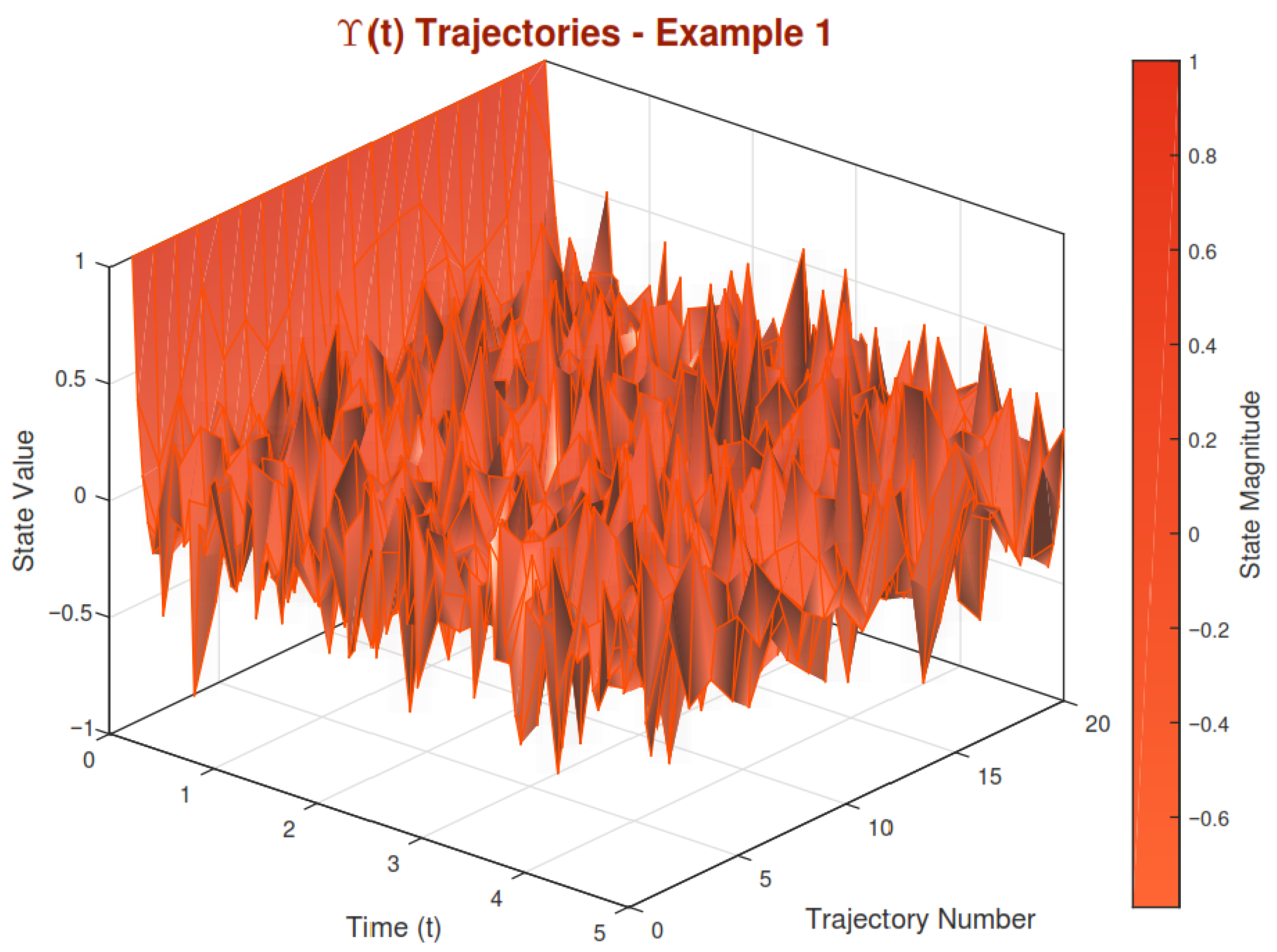
The Figure 1 and Figure 2 for the Ψ ( t ) and Υ ( t ) trajectories demonstrate the behavior of the linear coupled fractional stochastic system. Both variables exhibit smooth exponential decay due to negative eigenvalues ( A 1 = 2 , A 2 = 3 ) , with Ψ ( t ) starting at 2 and Υ ( t ) at 1. While Ψ ( t ) shows slightly wider variations due to noise, Υ decays faster and remains more tightly clustered, reflecting lower stochastic sensitivity. The blue Ψ ( t ) and red Υ ( t ) gradients highlight initial conditions fading over time, confirming the system’s mean-square Mittag-Leffler stability despite random perturbations.
Example 2. 
Consider the following nonlinear fractional neural hybrid stochastic system with ν = 2 3 :
D 0 + 2 / 3 ABC Ψ ( t ) + tanh ( Ψ ( t ) ) = Ψ ( t ) + | Υ ( t ) | 3 + d W ( t ) d t , D 0 + 2 / 3 ABC Υ ( t ) + tanh ( Υ ( t ) ) = Υ ( t ) + | Ψ ( t ) | 3 + d W ( t ) d t , Ψ ( 0 ) = 2 , Υ ( 0 ) = 1 ,
where W ( t ) are independent scalar Wiener processes.
We identify the system components as
A 1 = A 2 = 1 , g 1 ( t , Ψ ) = tanh ( Ψ ) , g 2 ( t , Υ ) = tanh ( Υ ) ,
F 1 ( t , Υ ) = | Υ | 3 , F 2 ( t , Ψ ) = | Ψ | 3 , σ 1 ( t , Ψ ) = σ 2 ( t , Υ ) = 1 .
The mild solution of system (24) is given by
Ψ ( t ) + tanh ( Ψ ( t ) ) = E 2 / 3 ( t 2 / 3 A 1 ) 2 + tanh ( 2 ) 0 t A 1 ( t δ ) 1 / 3 × E 2 / 3 , 2 / 3 ( ( t δ ) 2 / 3 A 1 ) tanh ( Ψ ( δ ) ) d δ + 0 t ( t δ ) 1 / 3 E 2 / 3 , 2 / 3 ( ( t δ ) 2 / 3 A 1 ) | Υ ( δ ) | 3 d δ + 0 t ( t δ ) 1 / 3 E 2 / 3 , 2 / 3 ( ( t δ ) 2 / 3 A 1 ) d W ( δ ) , Υ ( t ) + tanh ( Υ ( t ) ) = E 2 / 3 ( t 2 / 3 A 2 ) 1 + tanh ( 1 ) 0 t A 2 ( t δ ) 1 / 3 × E 2 / 3 , 2 / 3 ( ( t δ ) 2 / 3 A 2 ) tanh ( Υ ( δ ) ) d δ + 0 t ( t δ ) 1 / 3 E 2 / 3 , 2 / 3 ( ( t δ ) 2 / 3 A 2 ) | Ψ ( δ ) | 3 d δ + 0 t ( t δ ) 1 / 3 E 2 / 3 , 2 / 3 ( ( t δ ) 2 / 3 A 2 ) d W ( δ ) .
The nonlinear functions g 1 , g 2 and F 1 , F 2 satisfy CTC. They are measurable in t, continuous in state variables, and satisfy growth conditions via
| tanh ( Ψ ) | 1 , | x | 3 C ( 1 + | x | ) ,
ensuring non-Lipschitz but controlled growth.
The nonlinear integral equation
ν ( t ) = β 0 t ( ν ( δ ) ν ) d δ + ν ( 0 ) ,
admits a global solution by Peano-type existence theorems, as ν ( ν ) = C ( 1 + | ν | ) is continuous and sublinear.
All hypotheses H1–H5 in Theorem (3) are thus satisfied, and the system admits a unique mild solution on 1 2 , 1 . The linear operators A 1 = A 2 = 1 are negative definite. The nonlinearities satisfy growth conditions allowing for integral bounds in the stability estimate. The Lipschitz constants of σ i are bounded and continuous, i.e.,
E Ψ ( t ) 2 + E Υ ( t ) 2 C E 2 / 3 ( λ t 2 / 3 ) ,
for constants C , λ > 0 . Hence, by the stability result in Theorem (4), the solution ( Ψ ( t ) , Υ ( t ) ) is mean-square Mittag-Leffler stable. This guarantees long-term boundedness under stochastic perturbations, confirming the robustness of the solution.
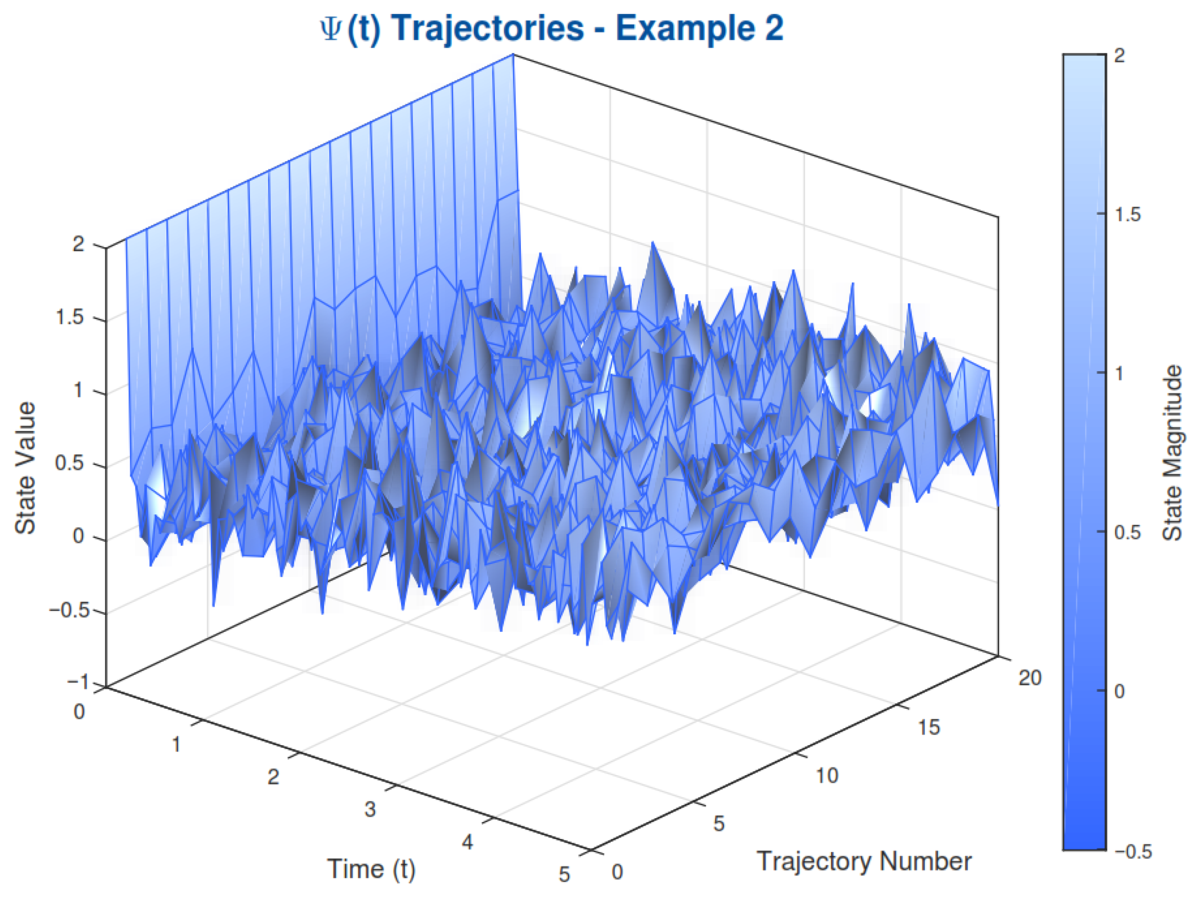
The nonlinear coupled system displays more complex dynamics, with Figure 3 and Figure 4 for Ψ and Υ trajectories showing irregular decay patterns influenced by tanh and cube root terms. Unlike the linear case, the paths exhibit intermittent plateaus and wider dispersion due to noise, particularly for Υ . The fractional-order memory effects are visible in the persistent correlations between states, while the ABC derivative ensures Mittag-Leffler-type stability. The plots illustrate how nonlinearities introduce richer behavior while maintaining overall stochastic stability.
Example 3. 
Consider the following nonlinear fractional hybrid stochastic coupled system with ν = 4 5 :
D 0 + 4 / 5 ABC Ψ ( t ) + 0.4 Ψ ( t ) cos ( Ψ ( t ) ) = A 1 ( r ( t ) ) Ψ ( t ) + B 1 tanh ( Υ ( t ) ) + σ 1 ( r ( t ) ) d W 1 ( t ) d t , D 0 + 4 / 5 ABC Υ ( t ) + 0.3 Υ ( t ) sin ( Υ ( t ) ) = A 2 ( r ( t ) ) Υ ( t ) + B 2 Ψ ( t ) e Ψ 2 ( t ) + σ 2 ( r ( t ) ) d W 2 ( t ) d t , Ψ ( 0 ) = 2.0 , Υ ( 0 ) = 1.0 ,
where r ( t ) is a continuous-time Markov chain taking values in { 1 , 2 } the with generator matrix
Q = 0.6 0.6 0.8 0.8 .
The mode-dependent parameters are
A 1 ( 1 ) = 3.0 , A 2 ( 1 ) = 2.5 , σ 1 ( 1 ) = 0.4 , σ 2 ( 1 ) = 0.3 , A 1 ( 2 ) = 1.2 , A 2 ( 2 ) = 1.0 , σ 1 ( 2 ) = 0.9 , σ 2 ( 2 ) = 0.7 ,
with coupling coefficients B 1 = 1.2 , B 2 = 0.9 . The mild solutions of the system are given by
Ψ ( t ) = E 4 / 5 t 4 / 5 A 1 ( r ( t ) ) [ 2.0 + 0.4 · 2.0 cos ( 2.0 ) ] 0.4 Ψ ( t ) cos ( Ψ ( t ) ) + 4 / 5 B ( 4 / 5 ) Γ ( 4 / 5 ) 0 t ( t δ ) 1 / 5 E 4 / 5 , 4 / 5 ( t δ ) 4 / 5 A 1 ( r ( δ ) ) × B 1 tanh ( Υ ( δ ) ) + σ 1 ( r ( δ ) ) W ˙ 1 ( δ ) d δ ,
Υ ( t ) = E 4 / 5 t 4 / 5 A 2 ( r ( t ) ) [ 1.0 + 0.3 · 1.0 sin ( 1.0 ) ] 0.3 Υ ( t ) sin ( Υ ( t ) ) + 4 / 5 B ( 4 / 5 ) Γ ( 4 / 5 ) 0 t ( t δ ) 1 / 5 E 4 / 5 , 4 / 5 ( t δ ) 4 / 5 A 2 ( r ( δ ) ) × B 2 Ψ ( δ ) e Ψ 2 ( δ ) + σ 2 ( r ( δ ) ) W ˙ 2 ( δ ) d δ .
g 1 ( t , Ψ ) g 1 ( t , Ψ ˜ ) = 0.4 Ψ cos Ψ Ψ ˜ cos Ψ ˜ 0.8 Ψ Ψ ˜ , g 2 ( t , Υ ) g 2 ( t , Υ ˜ ) = 0.3 Υ sin Υ Υ ˜ sin Υ ˜ 0.6 Υ Υ ˜ ,
with 0 < L 1 = 0.8 < 1 2 , 0 < L 2 = 0.6 < 1 2 .
F 1 ( t , Υ ) F 1 ( t , Υ ˜ ) = 1.2 tanh Υ tanh Υ ˜ 1.2 Υ Υ ˜ , F 2 ( t , Ψ ) F 2 ( t , Ψ ˜ ) = 0.9 Ψ e Ψ 2 Ψ ˜ e Ψ ˜ 2 0.9 Ψ Ψ ˜ , σ i ( t , Ψ ) σ i ( t , Υ ) L σ i Ψ Υ ,
satisfying the Lipschitz conditions.
F 1 ( t , 0 ) 2 + σ 1 ( t , 0 ) 2 ( 0 + 0 . 4 2 ) = 0.16 < , F 2 ( t , 0 ) 2 + σ 2 ( t , 0 ) 2 ( 0 + 0 . 3 2 ) = 0.09 < .
The matrices A 1 and A 2 are negative definite in both modes:
A 1 ( 1 ) x , x 3.0 x 2 , A 2 ( 1 ) x , x 2.5 x 2 , A 1 ( 2 ) x , x 1.2 x 2 , A 2 ( 2 ) x , x 1.0 x 2 .
The initial conditions are square-integrable: E 2.0 2 < , E 1.0 2 < . By Theorem 4, the mild solution ( Ψ ( t ) , Υ ( t ) ) is mean-square Mittag-Leffler-stable:
E Ψ ( t ) 2 + E Υ ( t ) 2 C E 4 / 5 ( λ t 4 / 5 ) ( E 2.0 2 + E 1.0 2 ) , t [ 0 , t ] .
All functions g i , F i , and σ i are measurable in t and continuous in the state variables. The drift terms satisfy
F 1 ( t , Υ ) 1.2 , F 2 ( t , Ψ ) 0.9 e 1 / 2 0.55 ,
ensuring controlled growth. The neutral terms satisfy g i ( t , x ) 0.4 x and g i ( t , x ) 0.3 x , respectively. The integral equation
ν ( t ) = β 0 t G ( δ , ν ( δ ) ) d δ + ν ( 0 ) ,
admits a global solution by Peano’s existence theorem, as the nonlinearities are continuous and sublinear. Therefore, by Theorem 3, the system admits a unique mild solution on 1 2 , 1 . In Figure 5 and Figure 6, we have presented three-dimensional plots for the concerned example.

6. Numerical Scheme: Adams–Bashforth Method for the ABC System

Consider the coupled stochastic fractional system in the Atangana–Baleanu–Caputo (ABC) sense, written in mild form:
X ( t ) = X 0 + 1 ν C ( ν ) F ( t , X ( t ) ) + ν C ( ν ) Γ ( ν ) 0 t ( t s ) ν 1 F ( δ , X ( δ ) ) d s + ν C ( ν ) Γ ( ν ) 0 t ( t s ) ν 1 Σ ( δ , X ( δ ) ) d W ( δ ) ,
where X = ( Ψ , Y ) , F is the drift vector, Σ is the diffusion vector, 0.5 < ν < 1 , and C ( ν ) is the ABC normalization constant.
Let the uniform grid be t n = n t for n = 0 , 1 , , N with t = T / N . Define
F j : = F ( t j , X j ) , Σ j : = Σ ( t j , X j ) , W j = W ( t j + 1 ) W ( t j ) .
The kernel weights for the fractional integral at t n + 1 are
w n + 1 , j = ( t n + 1 t j ) ν 1 , j = 0 , 1 , , n .
The fractional Adams–Bashforth (order–2) predictor is given by
X n + 1 pred = X 0 + 1 ν C ( ν ) F n + ν C ( ν ) Γ ( ν ) j = 0 n w n + 1 , j F ˜ j t + ν C ( ν ) Γ ( ν ) j = 0 n w n + 1 , j Σ j W j ,
where the modified values F ˜ j are defined by
F ˜ 0 = F 0 , F ˜ j = 3 2 F j 1 2 F j 1 , j 1 .
To improve stability and accuracy, a one–step Adams–Moulton corrector is applied using the predicted value:
X n + 1 = X 0 + 1 ν C ( ν ) F n + 1 pred + ν C ( ν ) Γ ( ν ) j = 0 n w n + 1 , j F j t + 1 2 w n + 1 , n F n + 1 pred t + ν C ( ν ) Γ ( ν ) j = 0 n w n + 1 , j Σ j W j + 1 2 w n + 1 , n Σ n + 1 pred W n .
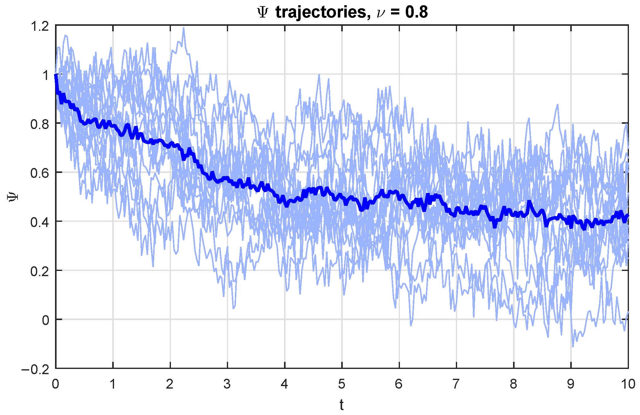
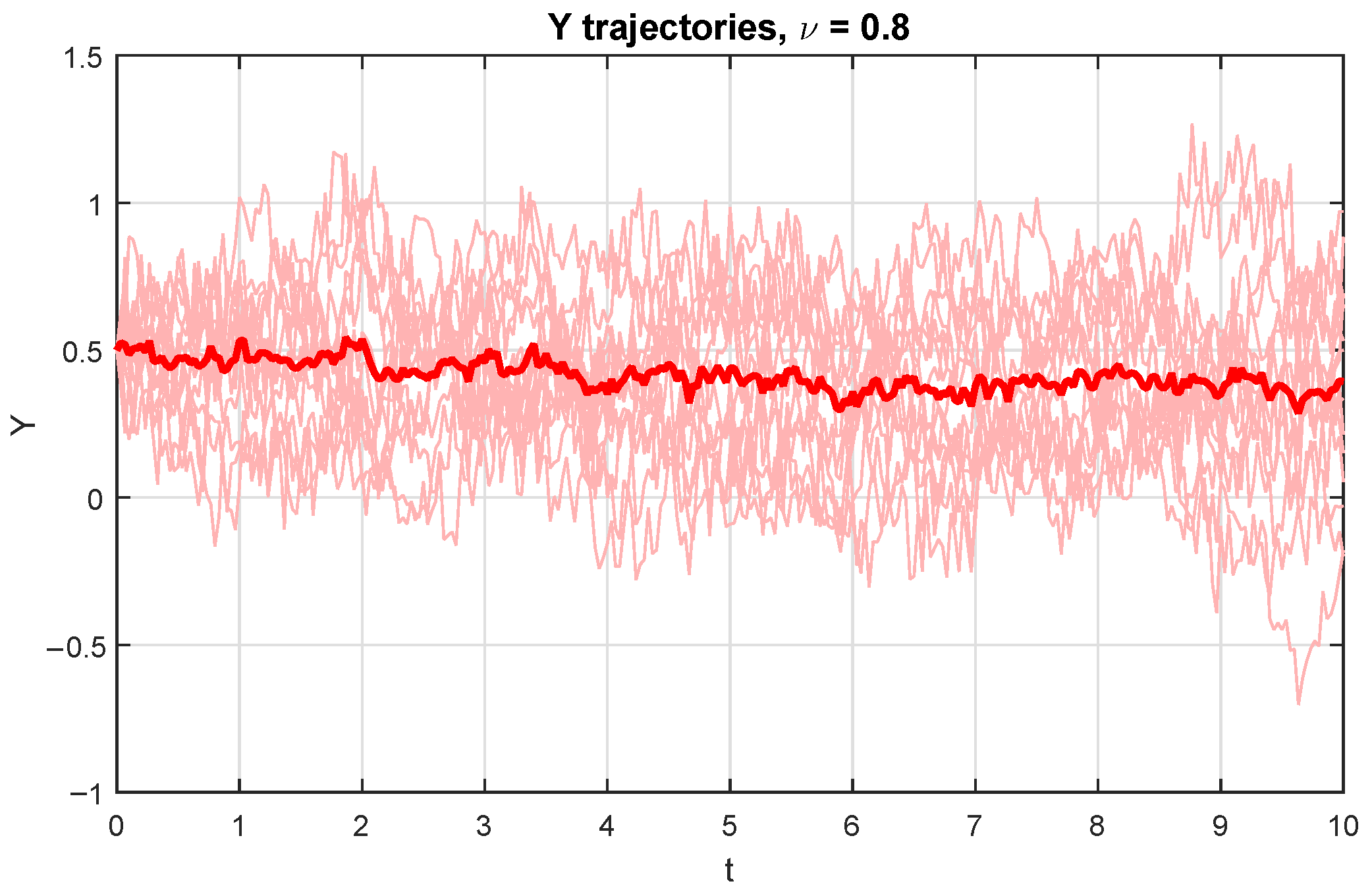
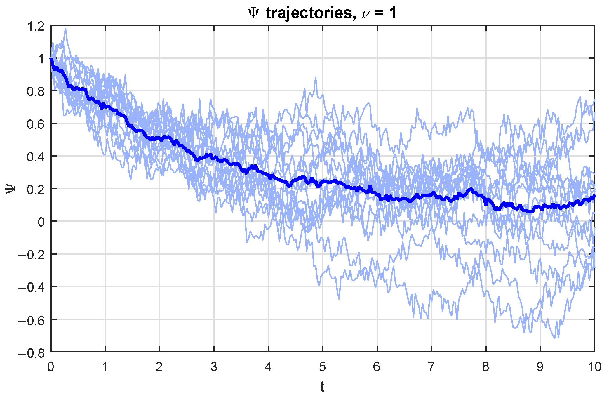
Figure 7 shows the trajectories of Ψ ( t ) , where the mean path (blue) remains stable with a narrow confidence band despite random fluctuations. Figure 8 presents the dynamics of Υ ( t ) , which exhibits higher variability but still converges around its mean (red). Both results confirm that the coupled system remains stable under stochastic and fractional effects.

7. Conclusions

In this article, we have proposed and investigated a novel class of nonlinear FSNHDE coupled systems based on the ABC derivative. The model accurately incorporates nonlocal memory effects, stochastic disturbances, and intercoupled subsystem interactions within a comprehensive framework. Based on the use of the non-singular Mittag-Leffler kernel, the ABC operator provides more accurate modeling of hereditary dynamics than traditional fractional models. The coupled structure also enhances modeling capability by capturing mutual influence and feedback among interdependent subsystems, such as neuron–glia interactions in neuroscience, temperature–humidity feedback cycles in climate models, and bidirectional actuator–sensor systems in engineering controls. By applying rigorous analysis, we proved the existence and uniqueness of mild solutions under Carathéodory-type assumptions, without imposing global Lipschitz continuity. The Picard successive approximation approach, in conjunction with integral kernel estimation, provides such systems with a strong theoretical basis. In addition to modeling flexibility, hybrid coupled systems offer significant benefits for real-world applications by allowing the concurrent representation of multiple dynamic agents that exhibit noise, memory, and switching behavior. The examples demonstrate that the theoretical findings are not only mathematically valid but also applicable to intricate dynamical systems found in bioengineering, smart grid control, epidemiological modeling, and viscoelastic material dynamics.
In summary, this study contributes to the growing body of literature on fractional stochastic dynamics and provides a flexible platform for further research in stability analysis, optimal control, numerical simulations, and delay-induced phenomena in practical hybrid systems.

Author Contributions

A Formal analysis, R.S.; Funding acquisition, A.H.A.A.; Investigation, R.S.; Project administration, K.A.; Resources, R.S.; Software, O.O.; Supervision, A.A.; Writing—original draft, J.A.; Writing—review & editing, A.H.A.A., K.A., A.A. and A.H.T. All authors have read and agreed to the published version of the manuscript.

Funding

This work was supported and funded by the Deanship of Scientific Research at Imam Mohammad Ibn Saud Islamic University (IMSIU) (grant number IMSIU-DDRSP2502).

Data Availability Statement

All data is included in the paper.

Conflicts of Interest

The authors declare no conflicts of interest.

References

  1. Kilbas, A.A.; Srivastava, H.M.; Trujillo, J.J. Theory and Applications of Fractional Differential Equations; Elsevier: Amsterdam, The Netherlands, 2006. [Google Scholar]
  2. Podlubny, I. Fractional Differential Equations:Fractional Differential Equations: An Introduction to Fractional Derivatives, Fractional Differential Equations, to Methods of their Solution and Some of Their Applications; Academic Press: Cambridge, MA, USA, 1998. [Google Scholar]
  3. Hamza, A.E.; Osman, O.; Ali, A.; Alsulami, A.; Aldwoah, K.; Mustafa, A.; Saber, H. Fractal-fractional-order modeling of liver fibrosis disease and its mathematical results with subinterval transitions. Fractal Fract. 2024, 8, 638. [Google Scholar] [CrossRef]
  4. Saber, H.; Almalahi, M.A.; Albala, H.; Aldwoah, K.; Alsulami, A.; Shah, K.; Moumen, A. Investigating a nonlinear fractional evolution control model using W-piecewise hybrid derivatives: An application of a breast cancer model. Fractal Fract. 2024, 8, 735. [Google Scholar] [CrossRef]
  5. Atangana, A.; Baleanu, D. New fractional derivatives with nonlocal and non-singular kernel: Theory and application to heat transfer model. Therm. Sci. 2016, 20, 763–769. [Google Scholar] [CrossRef]
  6. Jarad, F.; Uğurlu, E.; Abdeljawad, T.; Baleanu, D. On a new class of fractional operators. Adv. Differ. Equ. 2017, 2017, 247. [Google Scholar] [CrossRef]
  7. Mainardi, F. Fractional Calculus and Waves in Linear Viscoelasticity; World Scientific: Singapore, 2010. [Google Scholar]
  8. Øksendal, B. Stochastic Differential Equations: An Introduction with Applications; Springer: Berlin/Heidelberg, Germany, 2003. [Google Scholar]
  9. Mao, X. Stochastic Differential Equations and Applications; Horwood Publishing: Chichester, UK, 2007. [Google Scholar]
  10. Allen, L.J.S. An Introduction to Stochastic Processes with Applications to Biology; CRC Press: Boca Raton, FL, USA, 2007. [Google Scholar]
  11. Alqahtani, A.M.; Akram, S.; Ahmad, J.; Aldwoah, K.A.; Rahman, M.U. Stochastic wave solutions of fractional Radhakrishnan–Kundu–Lakshmanan equation arising in optical fibers with their sensitivity analysis. J. Opt. 2024. [Google Scholar] [CrossRef]
  12. Lu, W.; Ahmad, J.; Akram, S.; Aldwoah, K.A. Soliton solutions and sensitive analysis to nonlinear wave model arising in optics. Phys. Scr. 2024, 99, 085230. [Google Scholar] [CrossRef]
  13. Hale, J.K.; Verduyn Lunel, S.M. Dynamics and Delays; Springer: Berlin/Heidelberg, Germany, 2009. [Google Scholar]
  14. Lu, W.; Chen, G.; Cheng, D. Synchronization of coupled chaotic oscillators with time-varying delay. Chaos Solitons Fractals 2002, 14, 883–893. [Google Scholar]
  15. Liberzon, D. Switching in Systems and Control; Springer: Berlin/Heidelberg, Germany, 2003. [Google Scholar]
  16. Hale, J.K.; Verduyn Lunel, S.M. Introduction to Functional Differential Equations; Springer: Berlin/Heidelberg, Germany, 1993. [Google Scholar]
  17. Heemels, W.P.M.H.; De Schutter, B.; Van den Bosch, P.P.J. Hybrid dynamical systems: Modeling, stability, and robustness. Control Eng. Pract. 2009, 17, 1079–1087. [Google Scholar]
  18. Van der Schaft, A.; Schumacher, H. Introduction to Hybrid System Modeling and Control; Springer: Berlin/Heidelberg, Germany, 2000. [Google Scholar]
  19. Mao, X.; Yuan, C.G. Stochastic Differential Equations with Markovian Switching; Imperial College Press: London, UK, 1997. [Google Scholar]
  20. Yan, Y.; Zhang, H.; Sun, J.; Wang, Y. Sliding mode control based on reinforcement learning for TS fuzzy fractional-order multiagent system with time-varying delays. IEEE Trans. Neural Netw. Learn. Syst. 2023, 35, 10368–10379. [Google Scholar] [CrossRef]
  21. Angstmann, C.N.; Erickson, A.M.; Henry, B.I.; McGann, A.V.; Murray, J.M.; Nichols, J.A. Fractional-Order Compartment Models for Epidemic Spread. SIAM J. Appl. Math. 2017, 77, 430–446. [Google Scholar] [CrossRef]
  22. Monje, C.A.; Chen, Y.; Vinagre, B.M.; Xue, D.; Feliu, V. Fractional-Order Systems and Controls: Fundamentals and Applications; Springer: Berlin/Heidelberg, Germany, 2010. [Google Scholar]
  23. Chen, P.; Wang, B.; Tian, Y.; Yang, Y. Finite-time stability of a time-delay fractional-order hydraulic turbine regulating system. IEEE Access. 2019, 7, 82613–82623. [Google Scholar] [CrossRef]
  24. Dong, J.; Yang, Y. Hybrid Switching in Fractional-Order Neural Networks. Neural Netw. 2021, 133. [Google Scholar]
  25. Zhang, S.; Yu, Y.; Wang, H. Mittag-Leffler stability of fractional-order Hopfield neural networks. Nonlinear Analysis: Hybrid Systems. 2015, 16, 104–121. [Google Scholar] [CrossRef]
  26. Arnold, L. Stochastic Differential Equations: Theory and Applications; Wiley: Hoboken, NJ, USA, 1974. [Google Scholar]
  27. Yin, G.G.; Zhang, Q. Discrete-Time Markov Chains and Applications; Springer: Berlin/Heidelberg, Germany, 2002. [Google Scholar]
  28. Kushner, H.J. Stochastic Stability and Control; Academic Press: Cambridge, MA, USA, 1967. [Google Scholar]
  29. Khalil, H.K. Nonlinear Systems, 3rd ed.; Prentice Hall: Saddle River, NJ, USA, 2002. [Google Scholar]
  30. Banks, H.T.; Burns, J.A. Hereditary Control Problems: Numerical Methods Based on Averaging Approximations. SIAM J. Control Optim. 2006, 16, 169–208. [Google Scholar] [CrossRef]
  31. Kloeden, P.E.; Platen, E. Numerical Solution of Stochastic Differential Equations; Springer: Berlin/Heidelberg, Germany, 1992. [Google Scholar]
  32. Prato, G.D.; Zabczyk, J. Stochastic Equations in Infinite Dimensions; Cambridge University Press: Cambridge, UK, 1992. [Google Scholar]
  33. Mahmudov, N.I. Existence and uniqueness results for neutral SDEs in hilbert spaces. Stoch. Anal. Appl. 2007, 24, 79–95. [Google Scholar] [CrossRef]
  34. Govindan, T.E. Stability of mild solutions of stochastic evolution equations with variable delay. Stoch. Anal. Appl. 2003, 21, 1059–1077. [Google Scholar] [CrossRef]
  35. Taniguchi, T. Successive approximations to solutions of stochastic differential equations. J. Differ. Equ. 1992, 96, 152–169. [Google Scholar] [CrossRef]
  36. Yamada, T. On the successive approximation of solutions of stochastic differen- tial equations. J. Math. 1981, 21, 501–515. [Google Scholar]
  37. Rodkina, A.E. On existence and uniqueness of solution of stochastic differential equations with heredity. Stochastics 1984, 12, 187–200. [Google Scholar] [CrossRef]
  38. Balasubramaniam, P.; Vinayagam, D. Existence of solutions of nonlinear neu- tral stochastic differential inclusions in a hilbert space. Stoch. Anal. Appl. 2006, 23, 137–151. [Google Scholar] [CrossRef]
  39. Jiang, F.; Shen, Y. A note on the existence and uniqueness of mild solutions to neutral stochastic partial differential equations with non-Lipschitz coefficients. Comput. Math. Appl. 2011, 61, 1590–1594. [Google Scholar] [CrossRef]
  40. Govindan, T.E. Almost sure exponential stability for stochastic neutral partial functional differential equations. Stochastics 2005, 77, 139–154. [Google Scholar] [CrossRef]
  41. Ahmadova, A.; Mahmudov, N.I. Existence and uniqueness results for a class of fractional stochastic neutral differential equations. Chaos Solitons Fractals 2020, 139, 110253. [Google Scholar] [CrossRef]
  42. Atangana, A.; Gómez-Aguilar, J.F. Decolonisation of fractional calculus rules: Breaking commutativity and associativity to capture more natural phenomena. Eur. Phys. J. Plus 2018, 133, 166. [Google Scholar] [CrossRef]
  43. Gorenflo, R.; Kilbas, A.A.; Mainardi, F.; Rogosin, S.V. Mittag-Leffler Functions, Related Topics and Applications; Springer: Berlin/Heidelberg, Germany, 2014. [Google Scholar]
  44. Alghamdi, M.A.; El-Sayed, A.M.A.; El-Sayed, A.M.A. Mean-square stability of Riemann–Liouville fractional Hopfield’s neural networks with impulses at random times. Adv. Differ. Equ. 2021, 2021, 237. [Google Scholar] [CrossRef]
  45. Belhenniche, A.; Guran, L.; Benahmed, S.; Lobo Pereira, F. Solving nonlinear and dynamic programming equations on extended b-metric spaces with the fixed-point technique. Fixed Point Theory Algorithms Sci. Eng. 2022, 2022, 24. [Google Scholar] [CrossRef]
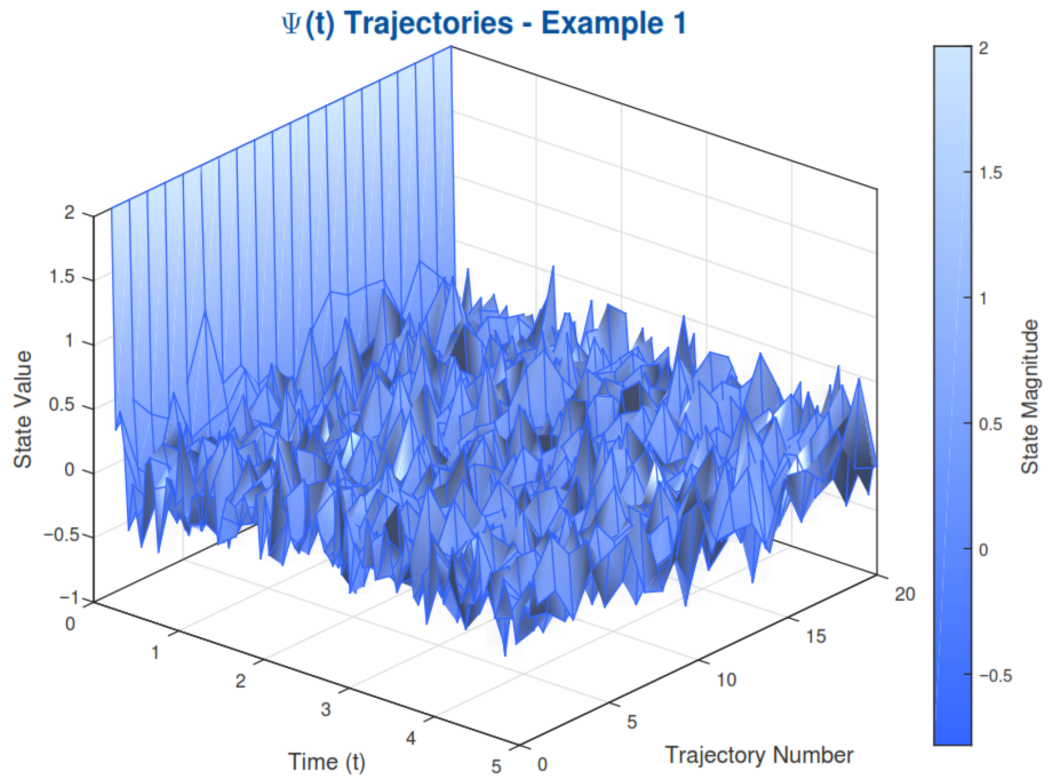
Figure 1. Three-dimensional plot for dynamic of Ψ ( t ) .
Fractalfract 09 00622 g001
Figure 2. Three-dimensional plot for dynamics of Υ ( t ) .
Fractalfract 09 00622 g002
Figure 3. Three-dimensional plot for dynamics of Ψ ( t ) .
Fractalfract 09 00622 g003
Figure 4. Three-dimensional plot for dynamics of Υ ( t ) .
Fractalfract 09 00622 g004
Figure 5. Three-dimensional plot. for dynamics of Ψ ( t ) .
Fractalfract 09 00622 g005
Figure 6. Three-dimensional plot. for dynamics of Υ ( t ) .
Fractalfract 09 00622 g006
Figure 7. Three-dimensional plot for dynamics of Ψ ( t ) .
Fractalfract 09 00622 g007
Figure 8. Three-dimensional plot for dynamics of Υ ( t ) .
Fractalfract 09 00622 g008
Disclaimer/Publisher’s Note: The statements, opinions and data contained in all publications are solely those of the individual author(s) and contributor(s) and not of MDPI and/or the editor(s). MDPI and/or the editor(s) disclaim responsibility for any injury to people or property resulting from any ideas, methods, instructions or products referred to in the content.