Analysis of Vehicle Vibration Considering Fractional Damping in Suspensions and Tires

Abstract

Vehicle dynamics play a crucial role in assessing vehicle performance, comfort, and safety. To precisely depict the dynamic behaviors of a vehicle, fractional damping is employed to substitute the conventional damping in suspensions and tires. Taking the fractional damping into account, a four-degrees-of-freedom vehicle model is developed, which encompasses the vertical vibration and pitch motion of the vehicle body, as well as the vertical motions of the front and rear axles. The vibration equations are solved in the Laplace domain using the transfer function method. The validity of the transfer function method is verified through comparison with a benchmark case. The vibrations of the vehicle are analyzed under the effects of suspension and tire properties, pavement excitation, and vehicle speed. The assessment methods employed include the time-domain vibration response, amplitude–frequency curves, phase diagrams, the frequency response function matrix, and weighted root mean square acceleration. The results show that the larger fractional order results in higher energy dissipation. Elevated values of the fractional order α, suspension stiffness, and the damping coefficient contribute to greater stable vibration amplitudes in vehicles and a consequent degradation in ride comfort. Higher tire stiffness reduces vehicle vibration amplitude, while the fractional order β and tire damping have a negligible effect. Moreover, increased vehicle speed and a greater pavement input amplitude adversely affect ride comfort.

1. Introduction

In recent years, the rapid advancement of the automobile industry has led to a substantial growth in vehicle ownership, making cars the increasingly chosen means of travel [1]. In the evaluation of vehicle performance, ride comfort and driving safety represent key metrics, for which vehicle dynamics is pivotal. Driving inevitably induces vibrations in vehicles, compromising both power efficiency and driving comfort through increased losses and reduced experience. As a result, vehicle dynamics has become a critical focus of research in automotive development [2].

Previous research on automotive vibrations includes modal analysis and experimental investigation, structural natural frequencies determinization [2], and nonlinear vibration analysis [3]. In recent years, propelled by advances in vibration theory and computer technology, research emphasis has shifted towards ensuring operational safety at higher vehicle speeds and exploring novel materials and structures for vibration and noise reduction [4]. Current research on automotive vibration primarily encompasses two major approaches: multi-degree-of-freedom (MDOF) dynamic equations for a vehicle system, and dynamic simulation based on commercial software [5].

A series of MDOF vehicle models were established in order to examine vibrational behavior under a range of operating conditions. The quarter-vehicle model, also known as the single-wheel model, represents the simplest approach for analyzing ride smoothness. This model accounts for two degrees of freedom: the vertical motion of both the vehicle body and a single wheel [6]. Common simplified vehicle dynamics models include the 2-DOF half-vehicle model, and more complex variants ranging from 4-DOF to 7-DOF whole-vehicle models, as well as 5-DOF half-vehicle models [2]. For example, Borowiec et al. [7] investigated a single-DOF nonlinear model focused on a quarter-car automobile with a semi-active nonlinear suspension. Türkay and Akçay [8] employed a single-DOF quarter-car model to study the vehicle’s response to a profile-imposed excitation, incorporating both a randomly varying traversal velocity and a variable vehicle forward speed. Liang et al. [9] used a 2-DOF nonlinear vehicle suspension model to analyze the chaotic vibration of a vehicle passing the consecutive speed control humps on a highway. Paliwal et al. [10] investigated the effect of varying road profile amplitude on the behavior of a nonlinear quarter-car model. Yang et al. [11] analyzed chaotic vibration and ride comfort in a vehicle passing consecutive speed control humps, using a 4-DOF half-vehicle model with a variable-frequency sine-trapezoidal wave excitation. Zhu et al. employed a 4-DOF half-vehicle model [12] and 7-DOF ground vehicle model [13] to investigate chaotic vibration while considering nonlinear spring and damping elements. To enhance the precision of automobile vibration analysis, researchers sometimes employ even more intricate vibration models [14]. However, increased model complexity can create some computational difficulties.

Vibration damping components, such as suspension systems and tires in automobiles, play an important role to ensure the ride comfort and safety of vehicles [15]. The suspension systems are usually characterized by using springs and dampers in lumped mass vehicle models with multiple DOFs [3]. A nonlinear damping model was proposed by Li et al. [16] to characterize hysteretic damping in intelligent vehicle suspension systems, incorporating smart fluids such as electro-rheological and magneto-rheological fluid dampers. Dobriyal [17] established a quarter-car model to analyze the dynamic behaviors of a passive suspension system with a power law spring. Abolfathi [18] examined the possibility of using a nonlinear Quasi-Zero-Stiffness spring in a vehicle suspension. Liang et al. [9] represented both the suspensions and tires with coupled nonlinear spring and damper elements. Zhu and Ishitobi’s MDOF vehicle model [13] used a set of nonlinear spring and damper elements for the suspensions and a nonlinear spring with a linear damper for the tires. These vibration damping components not only exhibit nonlinear characteristics of hysteresis, but also have viscoelastic characteristics that are intermediate between those of solids and liquids [19]. When describing the material properties of viscoelastic materials by integer-order calculus theory, it is often necessary to establish a complex model and obtain a large number of parameters in order to accurately describe their viscoelastic characteristics [20]. Since fractional calculus theory can well describe the properties of viscoelastic materials with few parameters [21,22,23], some researchers have applied the theory to the study of automobile suspensions. For example, Ullah et al. [24] investigated the chaotic vibration of a nonlinear suspension system with a fractional derivative. Tuwa et al. [25] studied the dynamical analysis of a quarter-car suspension based on the fractional Kelvin–Voigt viscoelastic model. Chang et al. [26] proposed a fractional nonlinear model of a 2-DOF quarter vehicle to investigate the dynamic behaviors of suspension systems. Watanabe et al. [27] proposed a fractional delayed feedback control for a semi-active suspension for a nonlinear jumping quarter-car model. Chen et al. [19] analyzed the stochastic bifurcation and dynamic reliability of a nonlinear MDOF vehicle system with generalized fractional damping. Molla et al. [28] analyzed the dynamic responses of quarter-car models with fractional-order damping. Yuvapriya et al. [29] investigated the vibration performance of the suspension using fractional-order synovial control in MATLAB/Simulink software (R2011a). However, these studies solely focused on the fractional damping enhancement within the automotive suspension component, without considering improvements to the vehicle tire damping under fractional calculus theory.

In recent years, the transfer function method in modeling viscoelastic behaviors has been popular [21,22]. This paper investigated the dynamic responses of a car with fractional damping both in the suspension and a tire. The rest of this paper is outlined as follows. In Section 2, the fractional damping element is introduced. In Section 3, the car dynamics are modeled based on fractional damping, and the transfer function method is validated. In Section 4, the effects of several factors on car dynamics are investigated. Some conclusions are presented in Section 5.

2. Fractional Damping Element

This section briefly introduces the theory of fractional calculus first. Then, the fractional damping elements and the fractional Kelvin (FK) model are established, and the mechanical behaviors of the FK model are analyzed with different parameters.

2.1. Theory of Fractional Calculus

Fractional calculus does not have a fixed definition, but the most commonly used ones are the Riemann–Liouville (RL) definition and the Caputo definition [20]. Both definitions have different application scenarios in physical and engineering problems. In this paper, the RL definition is adopted. The RL fractional integral is defined as follows:

$$I_b^{\alpha }f(t)={\displaystyle \frac{1}{\mathsf{\Gamma }(\alpha )}}{\displaystyle {\int }_b^t\frac{f(\tau )d\tau }{{(t-\tau )}^{1-\alpha }}}(t>b,\alpha >0)$$

(1)

where Γ(α) is the gamma function with a variable α, the RL fractional derivative can be defined by the following equation:

$$\begin{gathered} \begin{array}{cc}\hfill {}_a{}^{RL}D_t^{\alpha }f(t)& ={\left({\displaystyle \frac{d}{dt}}\right)}^n{I}_{a+}^{n-\alpha }f(t)\hfill \\ & ={\displaystyle \frac{1}{\mathsf{\Gamma }(n-\alpha )}}{\left({\displaystyle \frac{d}{dt}}\right)}^n{\displaystyle {\int }_a^t\frac{f(\tau )d\tau }{{(t-\tau )}^{\alpha -n+1}}}\hfill \end{array} \\ (n=\left|\alpha \right|+1,n-1\le \alpha <n,t>a) \end{gathered}$$

(2)

For 0 < α < 1, the RL fractional derivative is degenerated by the following equation:

$${}_a{}^{RL}D_t^{\alpha }f(t)={\displaystyle \frac{1}{\mathsf{\Gamma }(1-\alpha )}}{\displaystyle \frac{d}{dt}}{\displaystyle {\int }_a^t\frac{f(\tau )d\tau }{{(t-\tau )}^{\alpha }}}(t>a)$$

(3)

The following is a brief description of some simple, commonly used properties satisfied by RL fractional calculus.

(1)

Linear property

Fractional calculus is a linear operator that satisfies the principle of superposition. If f(t) is a continuous function and its fractional derivative $D_t^{\lambda -\beta }f(t)$ exists, then the following equation holds:

$${}_{0}D_t^{\lambda }{}_{0}D_t^{-\beta }f(t)={}_{0}D_t^{\lambda -\beta }f(t)(\lambda >0,\beta >0)$$

(4)

particularly,

$${}_{0}D_t^{\lambda }{}_{0}D_t^{-\lambda }f(t)=f(t)(\lambda >0)$$

(5)

(2)

Laplace transforms property

The Laplace transform of the RL fractional derivative is expressed as

$$L\left\{{}_a{}^{RL}D_t^{p}f(t);s\right\}=s^{p}F(s)-{\displaystyle \sum _{k=0}^{n-1}{s}^k{}_a{}^{RL}D_t^{p-k-1}f(t){|}_{t=0}}$$

(6)

For $0\le p<1$, the above equation can be simplified as

$$L\left\{{}_a{}^{RL}D_t^{p}f(t);s\right\}=s^{p}F(s)-{}_{a}D_t^{1-p}f(t){|}_{t=0}$$

(7)

2.2. Fractional Damping Elements

The traditional Kelvin viscoelastic model cannot reflect the real dynamic behaviors of advanced suspensions and tires [19] because of its simple structure. Although the model’s descriptive ability can be enhanced by series-parallel connection with numerous elements, the resultant increase in parameters complicates and challenges model analysis. Therefore, in this paper, the traditional damping element is replaced by a fractional damping element, as shown in Figure 1.

The force-displacement equation of the fractional damping element is written as

$$F=c{D}_t^{\alpha }y$$

(8)

where F represents force, y is displacement; c is the damping coefficient; α is the fractional order. When α equals 1, the fractional damping element is degenerated to the conventional damping element.

The fractional Kelvin model consists of a fractional damping element in series with a spring, and its constitutive relationship is expressed as

$$F=ky+c{D}_t^{\alpha }y$$

(9)

where k is the stiffness coefficient of spring. When α equals 1, the fractional Kelvin model transitions to the conventional Kelvin model.

Next, we change the value of k, c, and α of the fractional Kelvin model, and the corresponding force-displacement hysteresis curves are calculated by the GL fractional derivative [20], as shown in Figure 2.

From Figure 2a, it can be seen that the maximum tensile/compressive load value increases with k. It can be seen from Figure 2b that the larger c leads to the larger maximum tensile/compressive load value and the hysteresis loop area, which means a larger energy dissipation. Furthermore, it can be seen from Figure 2c that the larger α results in the larger hysteresis loop area, which indicates higher energy dissipation.

3. Modeling of Car Dynamics Based on Fractional Damping

3.1. Simplification of the Whole Car Dynamics Modeling

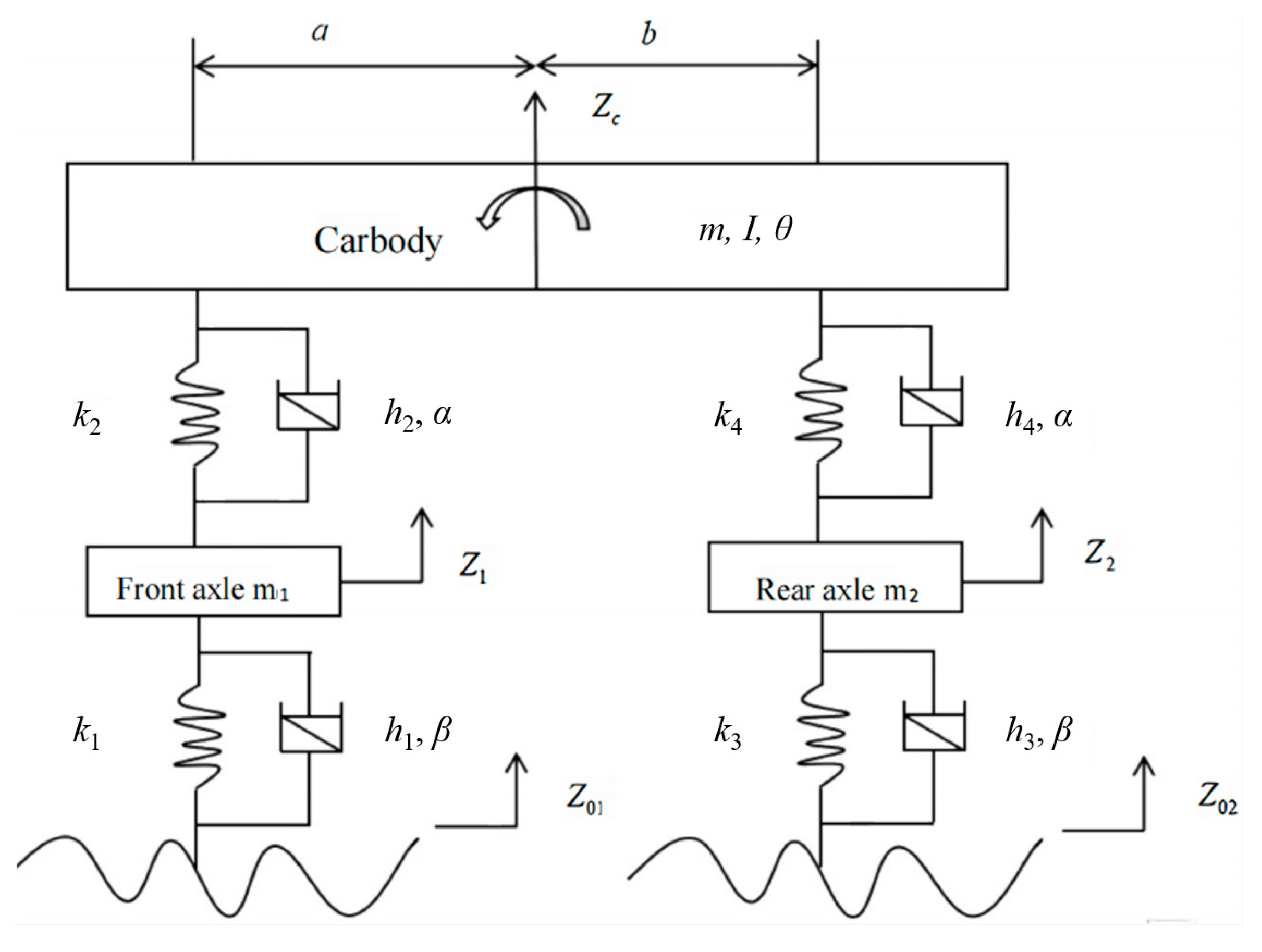
This paper employs an analytical approach that treats the vehicle as an integrated vibration system, comprising dampers, springs, and mass blocks. Given a vehicle symmetric about its longitudinal axis, vertical vibrations and pitching motions substantially influence driving stability and ride comfort. Accordingly, this study concentrates on the vertical vibration and pitch motion of the vehicle body, while also accounting for the vertical displacements of the front and rear axles. Furthermore, the analysis is confined to vibrations occurring in the longitudinal and vertical planes. The road surface is assumed to have unevenness only in the longitudinal direction, consistent with the direction of travel. Based on these assumptions, a four-degrees-of-freedom vehicle model is developed, as illustrated in Figure 3, with the corresponding parameters provided in

Table 1. Table of parameters involved in the diagram and the values [30].

Parameters	Physical Meaning	Unit	Values [30]
m	Car body mass	kg	1535
I	Vehicle body moment of inertia about the center of mass	kg·m2	17,577
m1	Front axle mass	kg	128
m2	Rear axle mass	kg	128
k1	Front tire stiffness	N·m−1	220,000
k2	Front suspension stiffness	N·m−1	22,741
k3	Rear tire stiffness	N·m−1	220,000
k4	Rear suspension stiffness	N·m−1	22,741
h1	Front tire damping	N·sβ·m−1	400
h2	Front suspension damping	N·sα·m−1	3800
h3	Rear tire damping	N·sβ·m−1	400
h4	Rear suspension damping	N·sα·m−1	4000
a	Distance from front axle to the center of mass	m	1.300
b	Distance from rear axle to the center of mass	m	1.705
α	Fractional order in suspensions	-
β	Fractional order in tires	-
zc	Vertical displacement of the car body	m
z1/z2	Axle vertical displacement	m
z01/z02	Pavement excitation input	m

.

3.2. Modeling of Pavement Irregularities’ Excitation Signals

In order to evaluate and improve the driving performance of a car, the dynamic response of the car is usually analyzed using road surface excitation signals. The pavement excitation signal is generated by the unevenness of the road surface, which has a direct impact on the driving comfort, maneuvering stability, ride quality, and the service life of the vehicle structure. By following Refs. [3,13,25], a sinusoidal road surface in the vertical direction is employed to characterize the road unevenness, as shown in Figure 4.

The differences in pavement excitation signals under different road conditions are mainly reflected in the frequency characteristics, amplitude, and vehicle speed. The relation between the pavement excitation amplitude and pavement position established in this paper is as follows:

$$y=A\sin Bx$$

(10)

where y is the height of the road surface, x represents the position of the road surface, A is the pavement input amplitude, and B = 2π/l, where l is the pavement input length representing the wavelength of the sinusoidal road surface. This study assumes that the vehicle travels at a constant speed in a straight line on the road surface. Therefore, the displacement–speed relationship is $x=vt$, where v is the speed of the car, and t is the driving time of car. Hence, the pavement excitation function at the rear axle can be rewritten as follows:

$$z_{01}=A\sin {\displaystyle \frac{2\pi vt}{l}}$$

(11)

Considering the distance a + b between the front and rear axles of the car, the pavement excitation function at the rear axle is expressed by

$$z_{02}=A\sin {\displaystyle \frac{2\pi v}{l}}\left(t+{\displaystyle \frac{a+b}{v}}\right)$$

(12)

In this paper, the vibration characteristics of the vehicle are analyzed mainly in terms of three differences between the pavement input length l, the pavement input amplitude A, and the vehicle speed v.

3.3. Derivation of Dynamical Equations with Fractional Damping Element

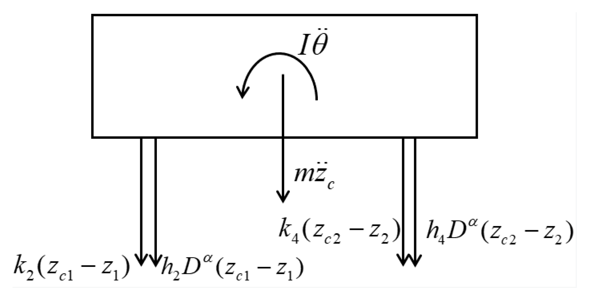
Based on the four-degrees-of-freedom dynamical model of the whole vehicle established in Section 3.1, the force analysis of the whole vehicle body is carried out, as shown in Figure 5.

The vehicle body is subjected to the downward elastic force of the two springs of the suspension and the damping force of the two suspension dampers, which are analyzed by D’Alembert’s principle:

$$m{\ddot{z}}_c+k_2(z_{c1}-z_1)+k_4(z_{c2}-z_2)+h_2{D}^{\alpha }(z_{c1}-z_1)+h_4{D}^{\alpha }(z_{c2}-z_2)=0$$

(13)

Moment equilibrium analysis of the center of mass of the car body from the above forces is written as follows:

$$I\ddot{\theta }+a{k}_2(z_{c1}-z_1)+a{h}_2{D}^{\alpha }(z_{c1}-z_1)-b{k}_4(z_{c2}-z_2)-b{h}_4{D}^{\alpha }(z_{c2}-z_2)=0$$

(14)

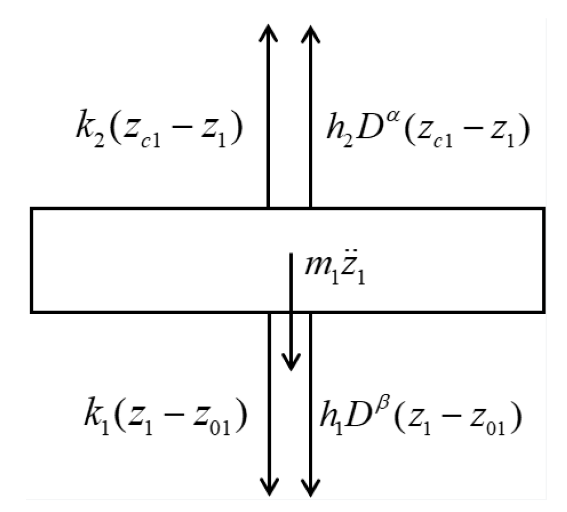
The resultant force acting on the vehicle’s front axle is analyzed in Figure 6. The front axle of the car is subjected to the upward tension of the suspension spring and the upward damping force of the suspension damping, as well as the downward spring force of the front wheel spring and the downward damping force of the front wheel damping, respectively, as analyzed by D’Alembert’s principle:

$$m_1{\ddot{z}}_1+k_1(z_1-z_{01})-k_2(z_{c1}-z_1)+h_1{D}^{\beta }(z_1-z_{01})-h_2{D}^{\alpha }(z_{c1}-z_1)=0$$

(15)

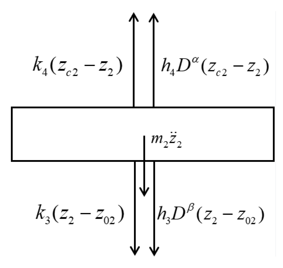
Similarly, Figure 7 illustrates the resultant forces acting on the rear-axle system. The rear axle of the car is subjected to the upward tension of the suspension spring and the upward damping force of the suspension damping, as well as the downward spring force of the rear wheel spring and the downward damping force of the rear wheel damping, respectively, as analyzed by D’Alembert’s principle:

$$m_2{\ddot{z}}_2+k_3(z_2-z_{02})-k_4(z_{c2}-z_2)+h_3{D}^{\beta }(z_2-z_{02})-h_4{D}^{\alpha }(z_{c2}-z_2)=0$$

(16)

According to the relationship between body and axle vertical displacement, it can be listed as follows:

$$z_{c1}=z_c-a\tan \theta$$

(17)

$$z_{c2}=z_c+b\tan \theta$$

(18)

Since the actual nodding motion of the car body is small, $\theta$ and $\tan \theta$ can be approximated to be equal, i.e., $\theta \approx \tan \theta$, which is obtained by taking into account the above two equations:

$$z_{c1}=z_c-a\theta$$

(19)

$$z_{c2}=z_c+b\theta$$

(20)

The vibration differential equation of the system can be obtained by organizing the above equation as follows:

$$m{\ddot{z}}_c+\left[k_2+k_4+\left(h_2+h_4\right)D^{\alpha }\right]z_c+\left[-a{k}_2+b{k}_4+\left(b{h}_4-a{h}_2\right)D^{\alpha }\right]\theta -(k_2+h_2{D}^{\alpha })z_1-(k_4+h_4{D}^{\alpha })z_2=0$$

(21)

$$I\ddot{\theta }+\left[a{k}_2-b{k}_4+\left(a{h}_2-b{h}_4\right)D^{\alpha }\right]z_c-\left[a^2{k}_2+b^2{k}_4+\left(a^2{h}_2+b^2{h}_4\right)D^{\alpha }\right]\theta -a\left(k_2+h_2{D}^{\alpha }\right)z_1+b\left(k_4+h_4{D}^{\alpha }\right)z_2=0$$

(22)

$$m_1{\ddot{z}}_1+\left(k_1+k_2+h_1{D}^{\beta }+h_2{D}^{\alpha }\right)z_1-\left(k_2+h_2{D}^{\alpha }\right)z_c+a\left(k_2+h_2{D}^{\alpha }\right)\theta =\left(k_1+h_1{D}^{\beta }\right)z_{01}$$

(23)

$$m_2{\ddot{z}}_2+\left(k_3+k_4+h_3{D}^{\beta }+h_4{D}^{\alpha }\right)z_2-\left(k_4+h_4{D}^{\alpha }\right)z_c-\left(k_4+h_4{D}^{\alpha }\right)b\theta =\left(k_3+h_3{D}^{\beta }\right)z_{02}$$

(24)

where the expressions of z₀₁ and z₀₂ can be referred to in Equations (11) and (12), respectively.

3.4. Transfer Function Representation of Vibration Response

Equations (21)–(24) can be transformed into algebraic equations by performing Laplace transforms assuming zero initial conditions:

$$\begin{array}{c}\left[k_2+k_4+\left(h_2+h_4\right)s^{\alpha }+m{s}^2\right]Z_c\left(s\right)+\left[-a{k}_2+b{k}_4+\left(b{h}_4-a{h}_2\right)s^{\alpha }\right]\mathsf{\Phi }\left(s\right)\\ -(k_2+h_2{s}^{\alpha })Z_1\left(s\right)-(k_4+h_4{s}^{\alpha })Z_2\left(s\right)=0\end{array}$$

(25)

$$\begin{array}{c}\left[a{k}_2-b{k}_4+\left(a{h}_2-b{h}_4\right)s^{\alpha }\right]Z_c\left(s\right)-\left[a^2{k}_2+b^2{k}_4+\left(a^2{h}_2+b^2{h}_4\right)s^{\alpha }+I{s}^2\right]\mathsf{\Phi }\left(s\right)\\ -a\left(k_2+h_2{s}^{\alpha }\right)Z_1\left(s\right)+b\left(k_4+h_4{s}^{\alpha }\right)Z_2\left(s\right)=0\end{array}$$

(26)

$$-\left(k_2+h_2{s}^{\alpha }\right)Z_c\left(s\right)+a\left(k_2+h_2{s}^{\alpha }\right)\mathsf{\Phi }\left(s\right)+\left(k_1+k_2+h_1{s}^{\beta }+h_2{s}^{\alpha }+m_1{s}^2\right)Z_1\left(s\right)={\displaystyle \frac{ABv\left(k_1+h_1{s}^{\beta }\right)}{s^2+B^2{v}^2}}$$

(27)

$$\begin{array}{c}-\left(k_4+h_4{s}^{\alpha }\right)Z_c\left(s\right)-b\left(k_4+h_4{s}^{\alpha }\right)\mathsf{\Phi }\left(s\right)+\left(k_3+k_4+h_3{s}^{\beta }+h_4{s}^{\alpha }+m_2{s}^2\right)Z_2\left(s\right)\\ ={\displaystyle \frac{A\left(k_3+h_3{s}^{\beta }\right)\left\{s\sin \left[B\left(a+b\right)\right]+Bv\cos \left[B\left(a+b\right)\right]\right\}}{s^2+B^2{v}^2}}\end{array}$$

(28)

where Z_c(s), Φ(s), Z₁(s), and Z₂(s) are the image functions of z_c(t), θ(t), z₁(t), and z₂(t) after Laplace transformation, respectively. Functions Z_c(s), Φ(s), Z₁(s), and Z₂(s) can be solved symbolically in MATLAB. After that, the numerical inverse Laplace transform [31] is taken to obtain the vibration responses in the time domain.

In addition, by replacing s with iω for Equations (25)–(28), the frequency response function (FRF) matrix of the system can be expressed by

$$H\left(\omega \right)={\left[M\left(\omega \right)\right]}^{-1}F\left(\omega \right)$$

(29)

where

$$M\left(\omega \right)=\left[\begin{array}{cccc}{k}_2+k_4+\left(h_2+h_4\right){\left(i\omega \right)}^{\alpha }-m{\omega }^2& -a{k}_2+b{k}_4+\left(b{h}_4-a{h}_2\right){\left(i\omega \right)}^{\alpha }& -(k_2+h_2{\left(i\omega \right)}^{\alpha })& -(k_4+h_4{\left(i\omega \right)}^{\alpha })\\ -a{k}_2+b{k}_4+\left(b{h}_4-a{h}_2\right){\left(i\omega \right)}^{\alpha }& a^2{k}_2+b^2{k}_4+\left(a^2{h}_2+b^2{h}_4\right){\left(i\omega \right)}^{\alpha }-I{\omega }^2& a\left(k_2+h_2{\left(i\omega \right)}^{\alpha }\right)& -b\left(k_4+h_4{\left(i\omega \right)}^{\alpha }\right)\\ -\left(k_2+h_2{\left(i\omega \right)}^{\alpha }\right)& a\left(k_2+h_2{\left(i\omega \right)}^{\alpha }\right)& k_1+k_2+h_1{\left(i\omega \right)}^{\beta }+h_2{\left(i\omega \right)}^{\alpha }-m_1{\omega }^2& 0\\ -\left(k_4+h_4{\left(i\omega \right)}^{\alpha }\right)& -b\left(k_4+h_4{\left(i\omega \right)}^{\alpha }\right)& 0& \left(k_3+k_4+h_3{\left(i\omega \right)}^{\beta }+h_4{\left(i\omega \right)}^{\alpha }-m_2{\omega }^2\right)\end{array}\right]$$

(30)

$$F\left(\omega \right)=\left[\begin{array}{cc}0& 0\\ 0& 0\\ k_1+h_1{\left(i\omega \right)}^{\beta }& 0\\ 0& k_3+h_3{\left(i\omega \right)}^{\beta }\end{array}\right]$$

(31)

3.5. Validation for Transfer Function Method

This section adopts a three-degrees-of-freedom free vibration benchmark problem, with a known analytical solution, to validate the transfer function method using a numerical inverse Laplace transform algorithm in [31]. The dynamic equation of a three-degrees-of-freedom system is written as

$$\left[\begin{array}{ccc}1& 0& 0\\ 0& 1& 0\\ 0& 0& 2\end{array}\right]\left\{\begin{array}{c}{\ddot{x}}_1\\ {\ddot{x}}_2\\ {\ddot{x}}_3\end{array}\right\}+\left[\begin{array}{ccc}2& -1& 0\\ -1& 2& -1\\ 0& -1& 1\end{array}\right]\left\{\begin{array}{c}{x}_1\\ x_2\\ x_3\end{array}\right\}=\left\{\begin{array}{c}0\\ 0\\ 0\end{array}\right\}$$

(32)

where x₁, x₂, and x₃ denote the displacements of the three degrees of freedom. The initial displacements and initial velocities are [0, 1] and [0, 0, 0], respectively. The analytical solution has been presented as [32]

$$x=\left\{\begin{array}{c}{x}_1\\ x_2\\ x_3\end{array}\right\}=\left\{\begin{array}{c}0.0595\\ 0.1059\\ 0.1467\end{array}\right\}\cos \left(0.3559t\right)+\left\{\begin{array}{c}0.5069\\ 0.3687\\ -0.2387\end{array}\right\}\cos \left(1.1281t\right)+\left\{\begin{array}{c}0.4345\\ -0.4783\\ 0.0919\end{array}\right\}\cos \left(1.7609t\right)$$

(33)

According to the transfer function methods, the displacements in the Laplace domain can be deduced by

$$\left\{\begin{array}{c}{X}_1\left(s\right)={\displaystyle \frac{s\left(2s^4+5s^2+1\right)}{2s^6+7s^4+4s^2}}\\ X_2\left(s\right)={\displaystyle \frac{s\left(2s^2+1\right)}{2s^6+7s^4+4s^2}}\\ X_3\left(s\right)={\displaystyle \frac{s}{2s^6+7s^4+4s^2}}\end{array}\right.$$

(34)

where X₁(s), X₂(s), and X₃(s) are the image functions of x₁(t), x₂(t), and x₃(t) in the Laplace domain. s is the complex variable. By taking the fast numerical inversion of Laplace transforms [31], the vibration responses for the three degrees of freedom can be calculated, which are compared with the corresponding analytical solutions, as shown in Figure 8. It can be seen from Figure 8 that the numerical results agree well with the analytical solutions. It validates the effectiveness of the transfer function method for simulating the vibration responses of a multi-degree-of-freedom system.

4. Results and Discussions

The parameters of a car are adopted from Ref. [30], as listed in Table 1. Substituting the parameters from Table 1 into the equations established in Section 3, vibration response curves are derived via inverse Laplace transform. These results undergo comprehensive analysis and discussion in the following section.

In this paper, the default value of l is set to be 5 m, A = 0.1 m, and vehicle speed v = 70 km/h for the sinusoidal excitation pavement. The fractional orders are set as α = 0.5, β = 0.5. The effects of suspensions, tires, pavement excitation, and car speed on vehicle vibration characteristics are comparatively analyzed in the following section.

4.1. Effect of Suspensions on Car Vibration

4.1.1. Fractional Order α

In this section, the effect of fractional order α in suspensions on car vibration is analyzed, where α = 0.3, 0.5, 0.7, and 1. The fractional order β in tires is set as 0.5. The vibration responses at different α are plotted in Figure 9, including the vertical vibration and pitch motion of the vehicle body.

It can be seen from Figure 9 that a higher fractional order α leads to shorter settling times for the vehicle to achieve steady-state periodic vibration, along with a larger stable peak amplitude. Compared with integer-order damping, fractional-order damping exhibits lower (stable) peak amplitudes but requires a longer settling time to reach steady-state vibration.

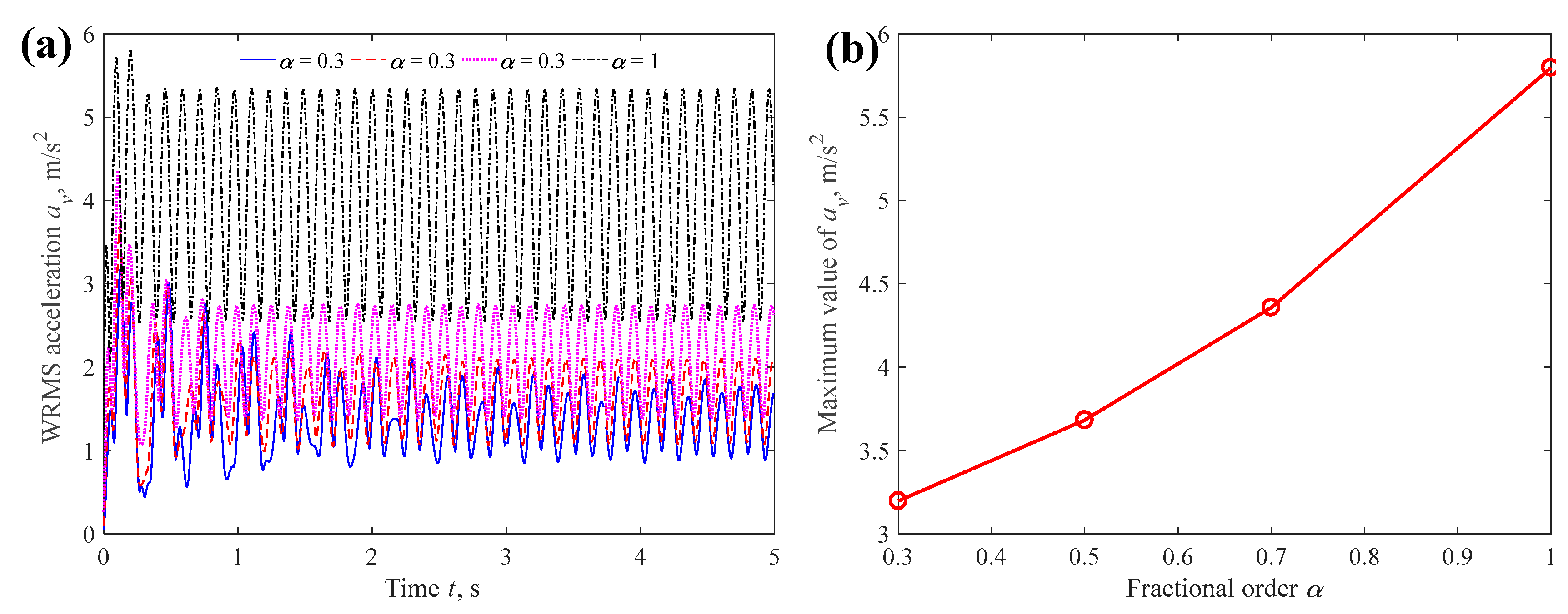
In order to evaluate the vibration comfort, we select the weighted root mean square (WRMS) acceleration a_v as the indicator for passenger comfort. A larger a_v value indicates worse comfort. The calculation formula for a_v is given as follows [33]:

$$a_v=\sqrt{{k_x}^2{a_{wx}}^2+{k_y}^2{a_{wy}}^2+{k_z}^2{a_{wz}}^2}$$

(35)

where a_wx, a_wy, and a_wz are the weighted root mean square accelerations along the orthogonal coordinate axes x, y, and z, respectively, and k_x, k_y, and k_z are the axis factors corresponding to the x-, y-, and z-axes. According to the four-degrees-of-freedom vibration model established in this study, lateral vibration in the y-direction is not considered, and the vertical vibration acceleration can be easily computed: $a_{wz}={\ddot{z}}_c$. Based on kinematic theory, the acceleration in the x-direction can be derived from the pitch angle and the x-direction distance L from the vehicle’s center of mass to the passenger [33]: $a_{wx}=\ddot{\theta }L$. The distance L is set as 1 m in this study. The weighted root mean square acceleration a_v can ultimately be expressed as follows:

$$a_v=\sqrt{{k_x}^2{(\ddot{\theta }L)}^2+{k_z}^2{{\ddot{z}}_c}^2}$$

(36)

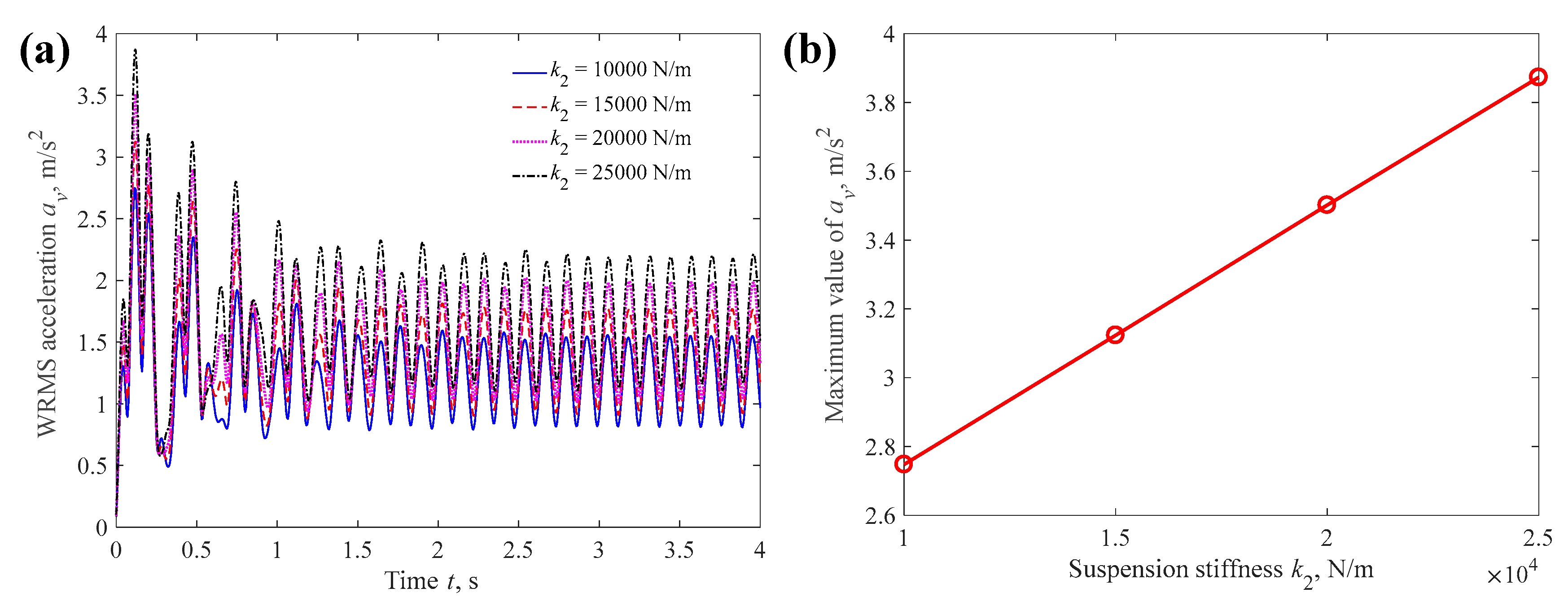
Following Ref. [33], the axis factors are taken as k_x = 1.4 and k_z = 1.0. Therefore, the time-dependent a_v and its maximum values for different fractional orders can be calculated, as shown in Figure 10. The results show that a larger fractional order leads to larger WRMS acceleration, which indicates a deterioration in ride comfort. Furthermore, fractional damping offers superior ride comfort compared to integer-order damping.

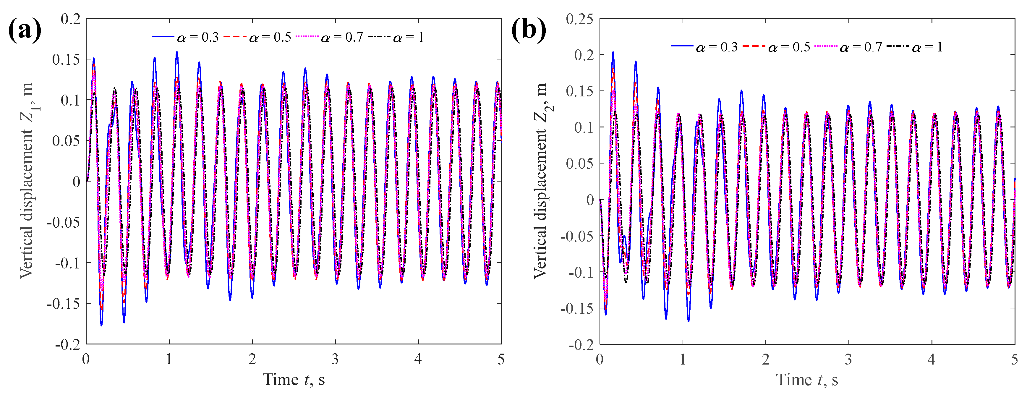
The vibration responses of axles at different α are also plotted in Figure 11. It can be observed that fractional order α has a certain influence on the transient vibration of the axles, whereas its effect on stable vibration is minimal.

4.1.2. Suspension Stiffness

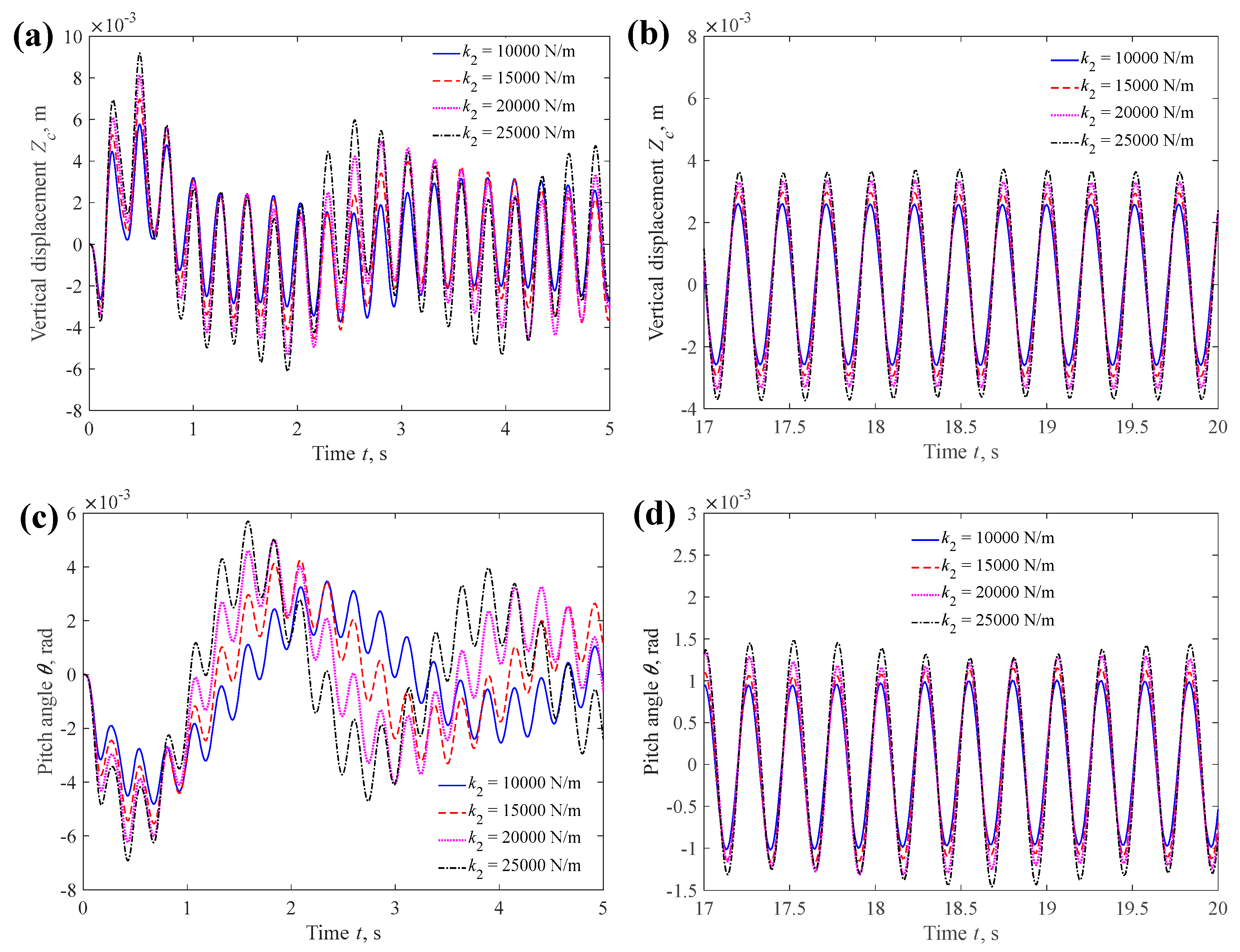
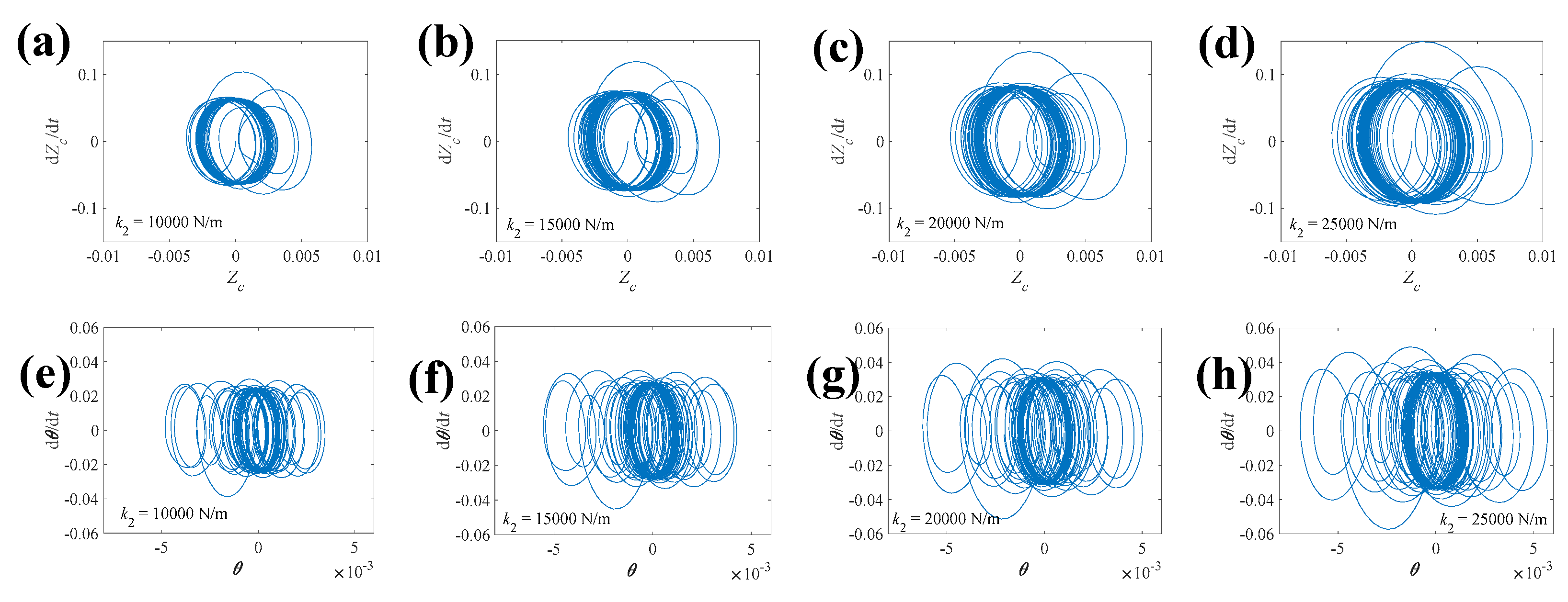
In this section, the effect of suspension stiffness k₂ or k₄ on car vibration is analyzed, where α = 0.5, and β = 0.3. Suspension stiffness k₂ or k₄ is set as 10,000, 15,000, 20,000, and 25,000 N·m⁻¹. The vibration responses at different suspension stiffnesses are plotted in Figure 12, including the vertical vibration and pitch motion of the vehicle body. The phase diagrams of the vehicle body at different suspension stiffnesses are also given in Figure 13. It can be seen from Figure 12 and Figure 13 that after irregular transient vibration, vibration tends to stabilize. Moreover, the higher suspension stiffness leads to a larger stable vibration amplitude.

The time-dependent a_v and its maximum values for different suspension stiffnesses are calculated, as shown in Figure 14. The results show that WRMS acceleration reaches a relatively high value initially, then decreases, and gradually stabilizes. A larger suspension stiffness results in larger WRMS acceleration, which indicates a deterioration in ride comfort. Moreover, the value of a_v exhibits a nearly linear increase with suspension stiffness.

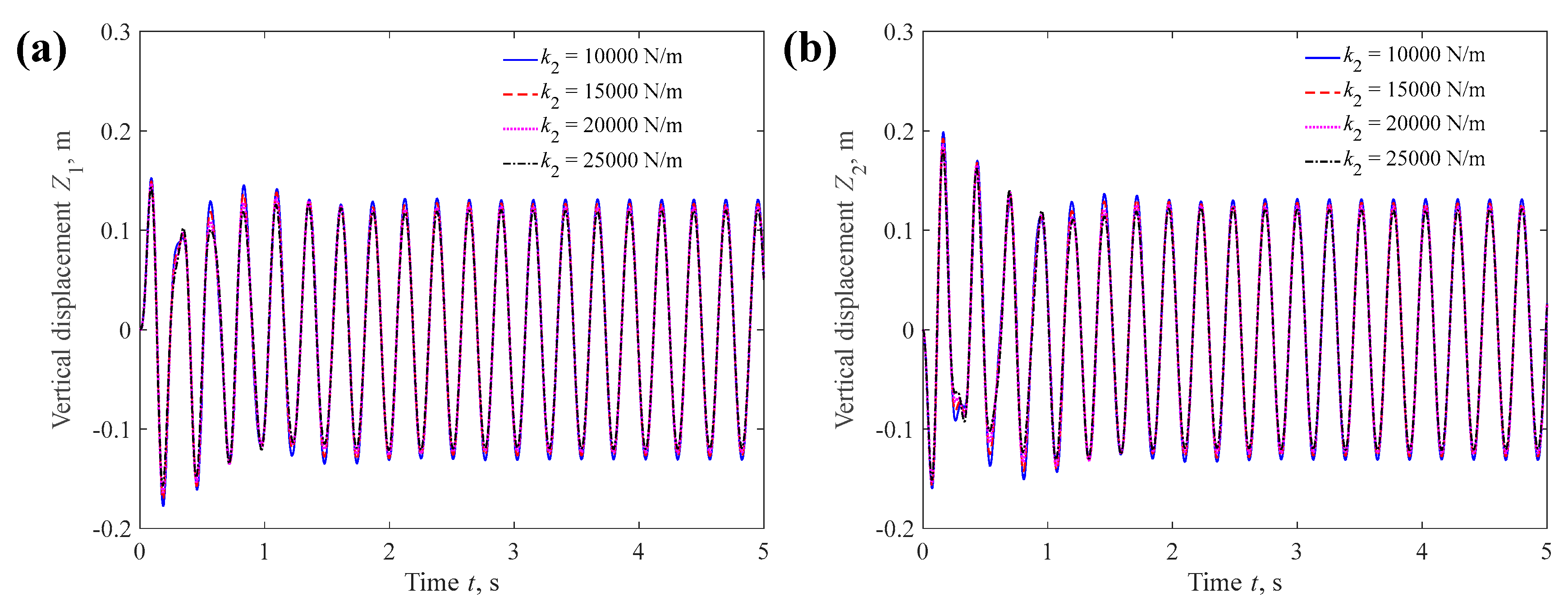
The vibration responses of axles at different suspension stiffnesses are also plotted in Figure 15. The results indicate that the effect of suspension stiffness on the vibration of axles can be ignored.

4.1.3. Suspension Damping

In this section, the effect of suspension damping h₂ or h₄ on car vibration is analyzed, where α = 0.5, and β = 0.3. Suspension damping h₂ or h₄ is set as 1000, 3000, 5000, and 7000 N·s^α·m⁻¹. Damping h₂ and h₄ are assumed to be equal. The vibration responses at different suspension damping amounts are plotted in Figure 16, including the vertical vibration and pitch motion of the vehicle body. From Figure 16, it can be seen that small suspension damping can lead to violent fluctuations in vibration amplitude for both vertical and pitch motions. A smaller damping coefficient leads to a reduced stable vibration amplitude at the expense of a longer settling time.

The time-dependent a_v and its maximum values for different suspension damping amounts are calculated, as shown in Figure 17. The results show that WRMS acceleration reaches a relatively high value initially, then decreases, and gradually stabilizes. A larger suspension damping amount results in larger WRMS acceleration, which indicates a deterioration in ride comfort. Moreover, the value of a_v exhibits a nearly linear increase with suspension damping. Consequently, the findings in Figure 16 and Figure 17 suggest that an optimal value for suspension damping exists, balancing the trade-off between passenger ride comfort and the rapid attainment of stable vibration modes.

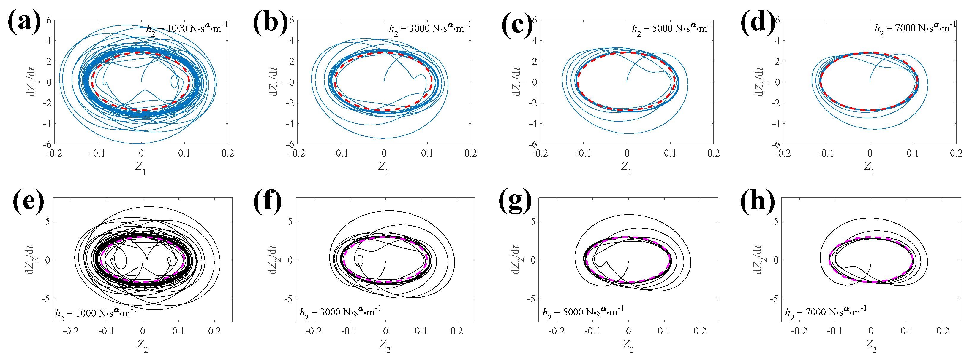
The phase diagrams of axles at different suspension damping amounts are also plotted in Figure 18. The results show that a smaller suspension damping amount leads to more time to reach a stable vibration of the axles. Additionally, the high suspension damping amount slightly reduces the stable vibration amplitude of the axles. According to the findings in Figure 16 and Figure 18, the effects of suspension damping on the vehicle body and axles are opposite. Therefore, for optimal ride comfort, the suspension damping amount should be as low as possible without compromising the rapid settling of vibrations.

4.2. Effect of Tires on Car Vibration

4.2.1. Fractional Order β

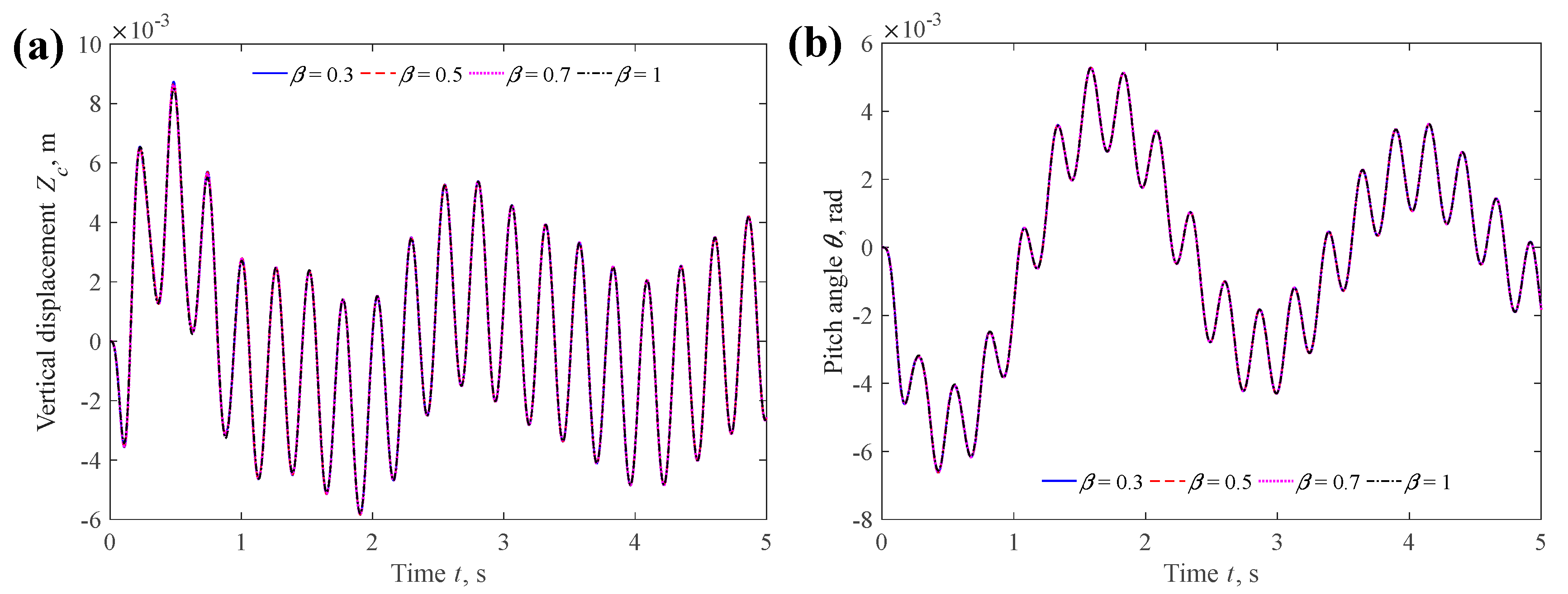
In this section, the effect of fractional order β in tires on car vibration is analyzed, where β = 0.3, 0.5, 0.7, and 1. The fractional order α in tires is set as 0.5. The vibration responses at different β are plotted in Figure 19 and Figure 20, including the vertical vibration and pitch motion of the vehicle body, and axle vertical vibration responses. As shown in Figure 19 and Figure 20, the influence of β on car body vibration is minimal. This phenomenon can be explained by the significantly lower tire damping coefficient (~400) relative to its stiffness (~220,000), as listed in Table 1.

4.2.2. Tire Stiffness

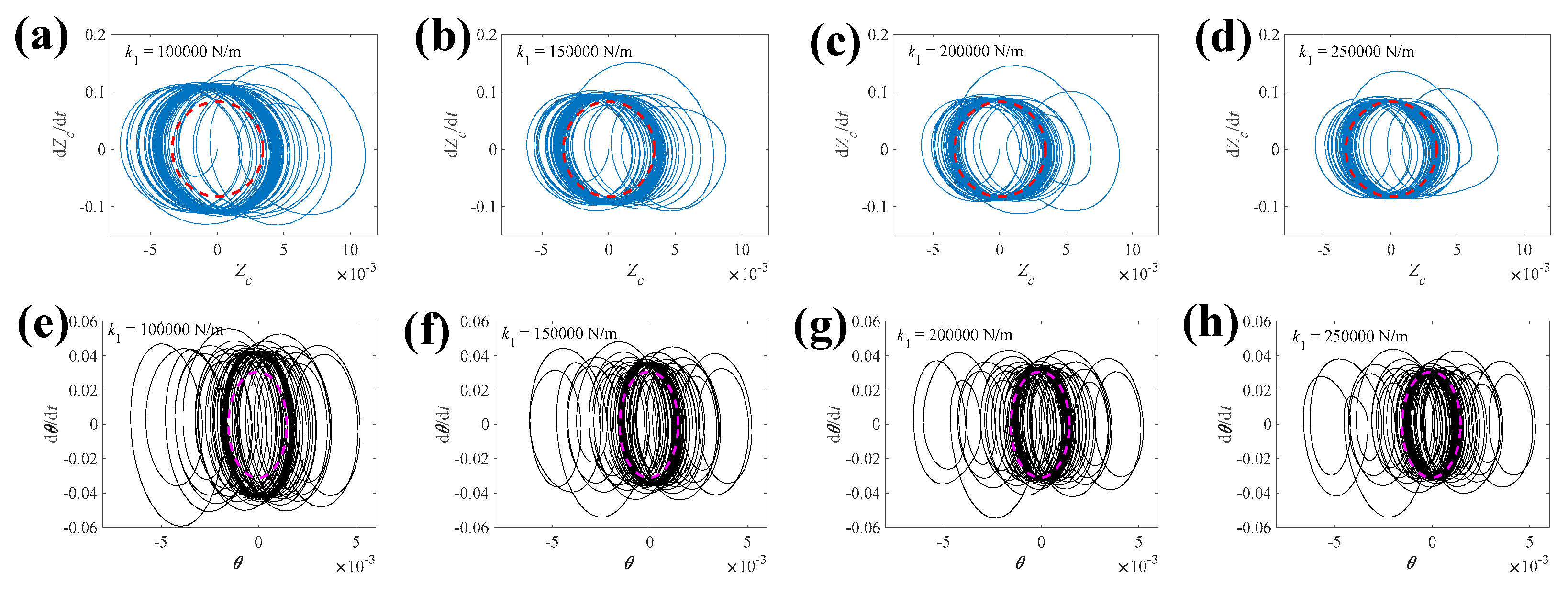
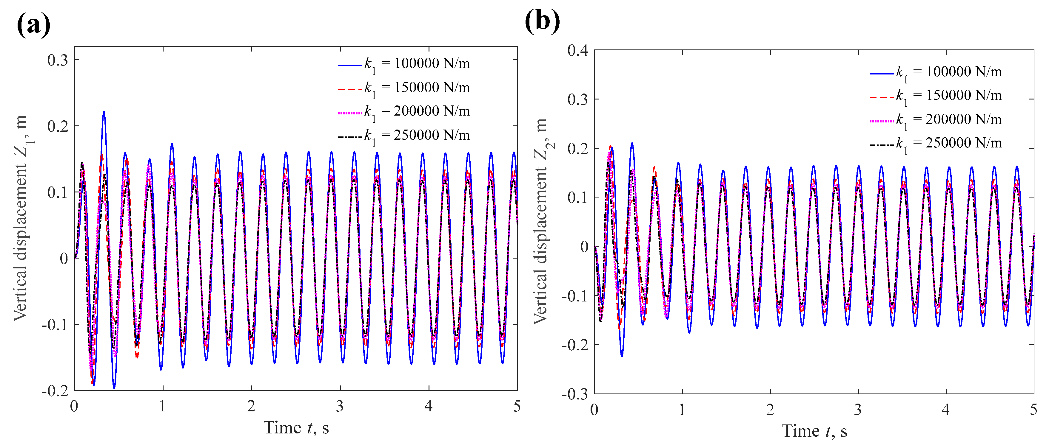
In this section, the effect of tire stiffness k₁ or k₃ on car vibration is analyzed, where α = 0.5, and β = 0.3. Tire stiffness k₁ or k₃ is set as 100,000, 150,000, 200,000, and 250,000 N·m⁻¹. The vibration responses at different tire stiffnesses are plotted in Figure 21, including the vertical vibration and pitch motion of vehicle body, and the axle vertical vibration response. The phase diagrams of vehicle body vibrations at different tire stiffnesses are plotted in Figure 22. From Figure 21 and Figure 22, it can be seen that a high tire stiffness can slightly reduce the vibration amplitude of the vehicle body.

The time-dependent a_v and its maximum values for different tire stiffnesses are calculated, as shown in Figure 23. The results show that WRMS acceleration reaches a relatively high value initially, then decreases, and gradually stabilizes. The WRMS acceleration initially decreases then increases with higher tire stiffness, suggesting the existence of an optimal value that minimizes the WRMS acceleration for optimal ride comfort.

The vibration responses of axles at different tire stiffnesses are plotted in Figure 24. It shows that the larger tire stiffness leads to the smaller vibration amplitude of the axles.

4.2.3. Tire Damping

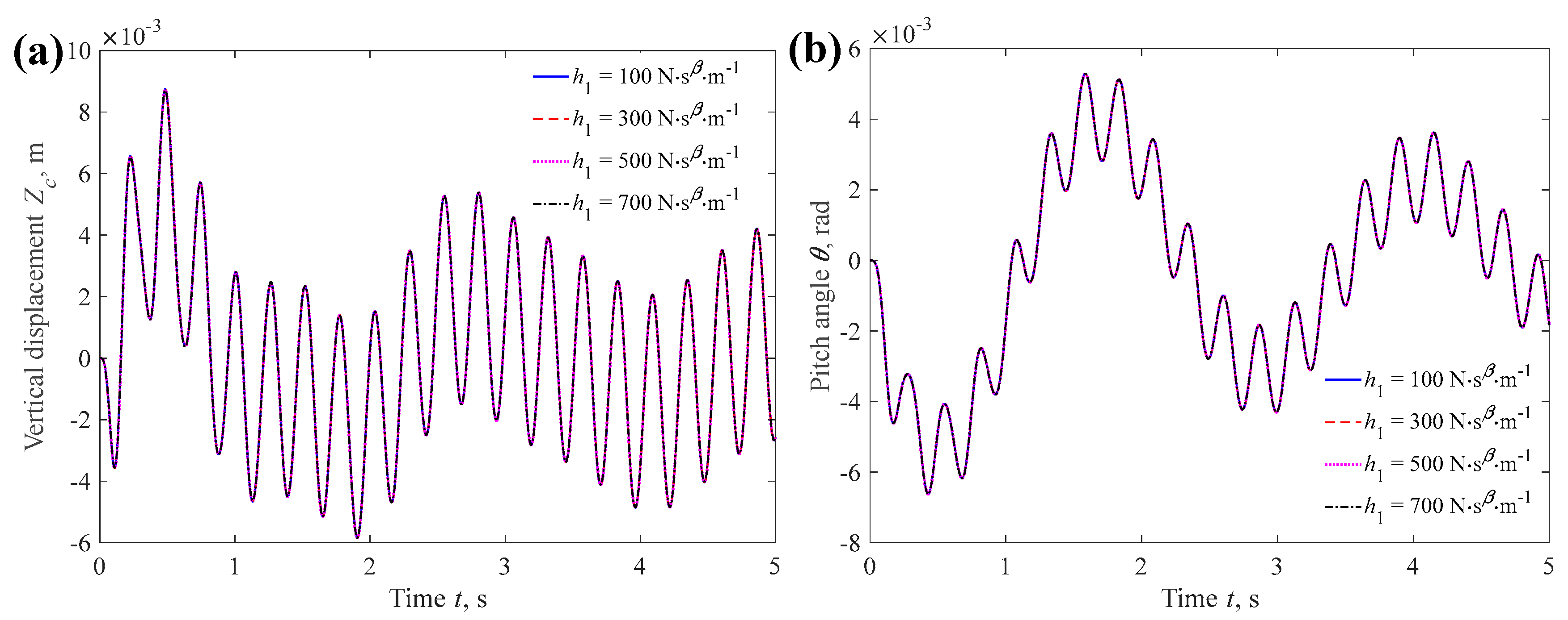
In this section, the effect of tire damping h₁ or h₃ on car vibration is analyzed, where α = 0.5, and β = 0.3. Tire damping h₁ or h₃ is set as 100, 300, 500, and 700 N·s^β·m⁻¹. The vibration responses at different tire damping amounts are plotted in Figure 25 and Figure 26, including the vertical vibration and pitch motion of vehicle body, and the axle vertical vibration response. The results indicate that tire damping has minimal influence on vehicle vibration. This is likely due to the considerable difference (approximately three orders of magnitude) between the tire’s damping coefficient (~400) and its stiffness (~220,000), as provided in Table 1.

4.3. Effects of Pavement Excitation and Car Speed on Car Vibration

4.3.1. Car Speed

In this section, vibration characteristics of the vehicle are analyzed across different speeds (50, 70, 100, and 120 km/h) under uniform linear motion conditions. With fixed parameters at A = 0.1 m and l = 5 m, speed serves as the single variable for comparison. Control tests are conducted for four distinct speed cases. The fractional orders are set as α = 0.5, and β = 0.5. The resulting MATLAB simulations are shown below.

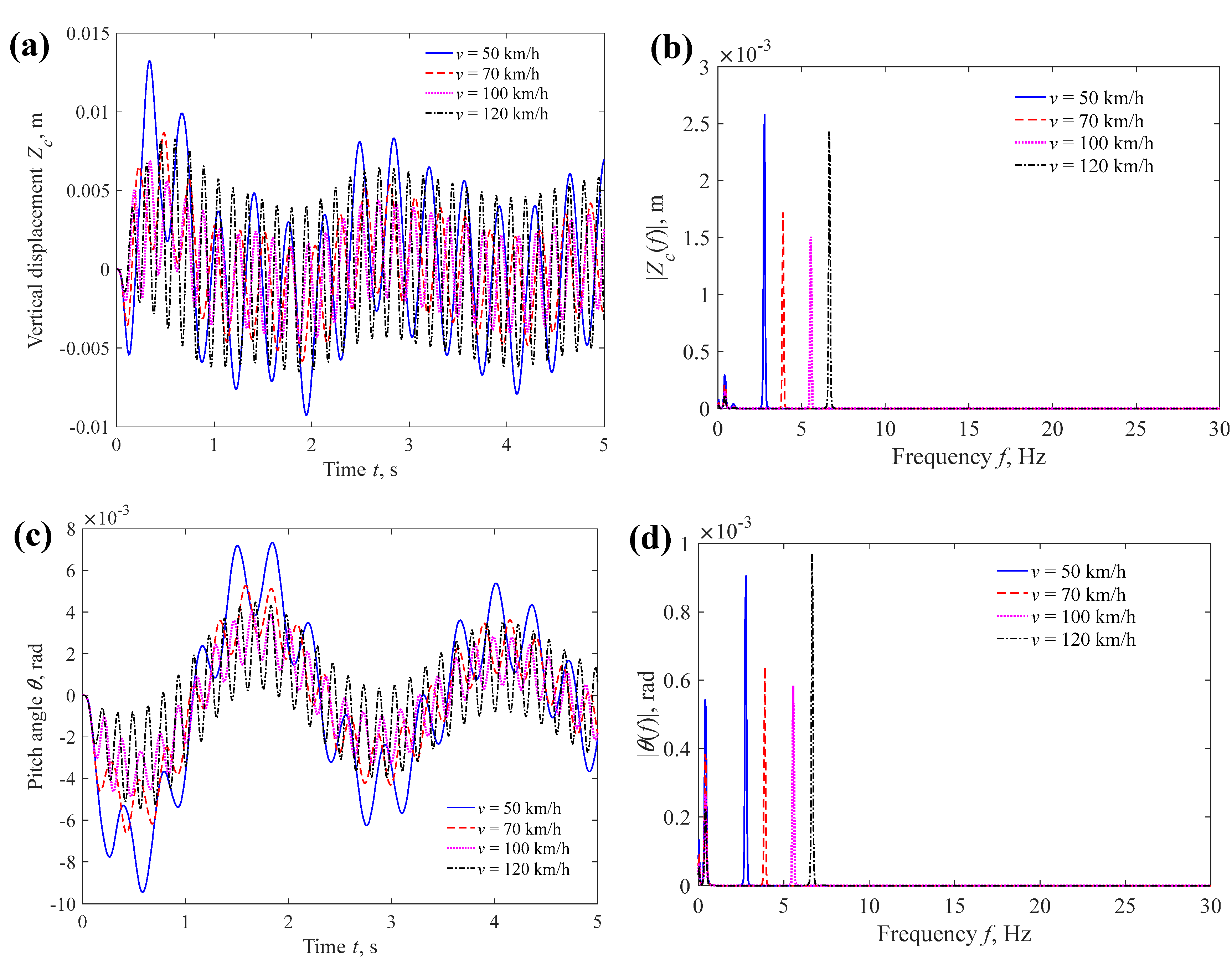
The vertical vibration and pitch motion of the vehicle body at different speeds are plotted in Figure 27a,c. The amplitude–frequency curve, obtained by converting time-domain data via the Fast Fourier Transform (FFT) method, is presented in Figure 27b,d. As shown in Figure 27, the initial vibrations exhibit chaotic behavior. The amplitude–frequency response further indicates that the stable vibration amplitude of the vehicle body first decreases and then increases with rising vehicle speed.

According to Figure 27b,d, the excitation frequencies at vehicle speeds of 50, 70, 100, and 120 km/h are 2.78 Hz, 3.89 Hz, 5.56 Hz, and 6.67 Hz, respectively. Moreover, based on the frequency response function (FRF) matrix given in Equation (29) and the parameters listed in Table 1 and this section, the natural frequencies of the vehicle system are numerically calculated as 0.93 Hz and 7.5 Hz, as illustrated in Figure 28.

Therefore, it can be concluded that the high vibration amplitude of the vehicle body at speeds of 50 km/h and 120 km/h results from the excitation frequencies being close to the system’s natural frequencies.

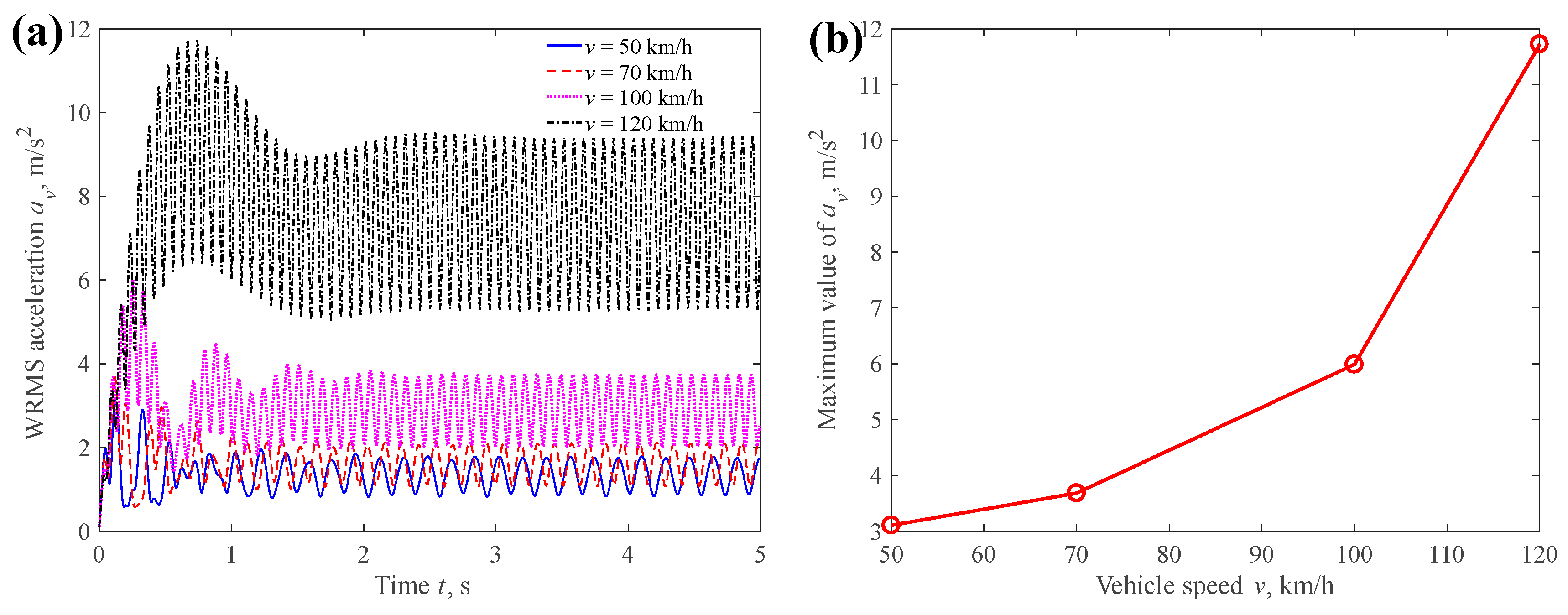
Furthermore, the WRMS accelerations at various vehicle speeds were calculated to evaluate vibration comfort. Figure 29 reveals that acceleration exhibits a near-linear increase with vehicle speed. This trend shows a rapid deterioration in ride comfort as speed increases.

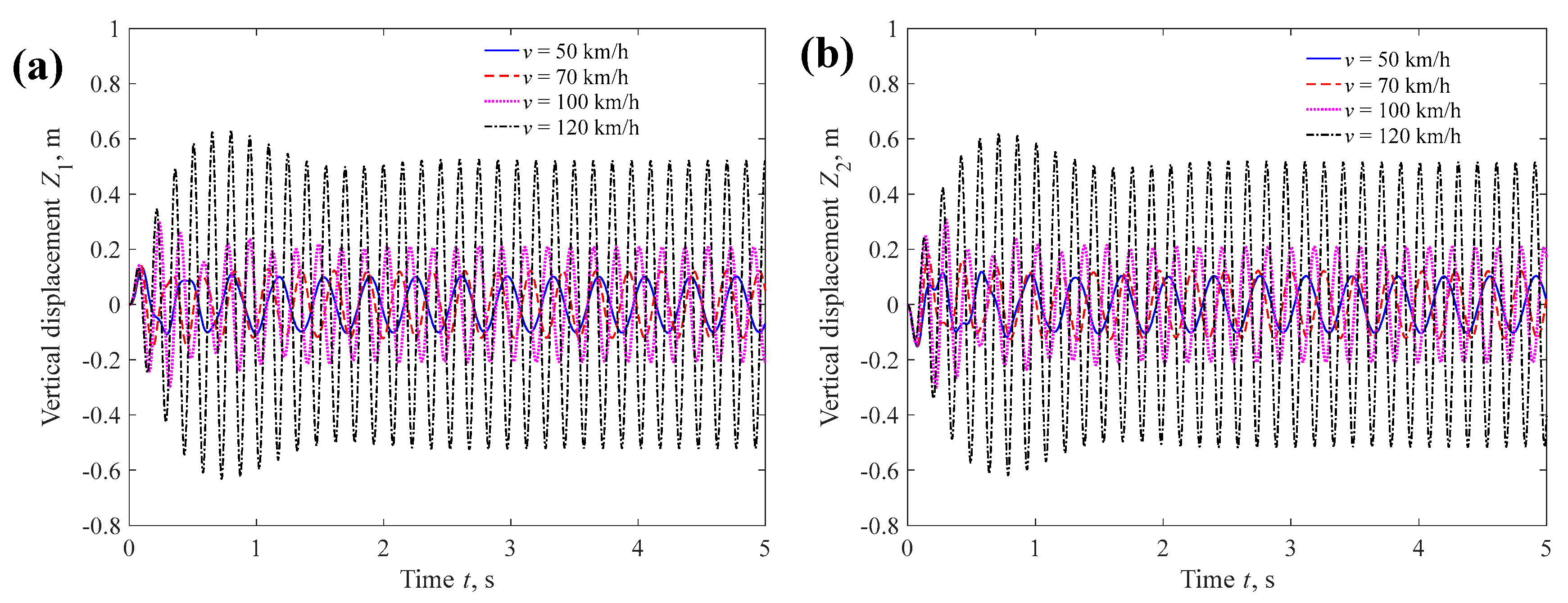
The axle vertical vibration responses at different speeds are plotted in Figure 30. It can be observed that the larger vehicle speed results in the larger axle vibration amplitude. Therefore, based on the analysis of Figure 27, Figure 28, Figure 29 and Figure 30, vehicle speed should be controlled within a safe range to ensure both safety and comfort.

4.3.2. Pavement Input Amplitude

This section analyzes the vibration characteristics of the vehicle traveling at a constant speed of 70 km/h over a sinusoidal road profile with a wavelength (l) of 5 m. Pavement input amplitudes of A = 0.03 m, 0.05 m, 0.1 m, and 0.2 m are simulated to investigate the response. The fractional orders are set as α = 0.5 and β = 0.5.

The vibration responses of the car body for different road input amplitudes are shown in Figure 31. The result in Figure 31a indicates that as the amplitude of road surface excitation increases, the vertical vibration amplitude of the vehicle body exhibits a significant upward trend. Figure 31b shows that the higher road input amplitudes correspond to larger pitch motion amplitudes.

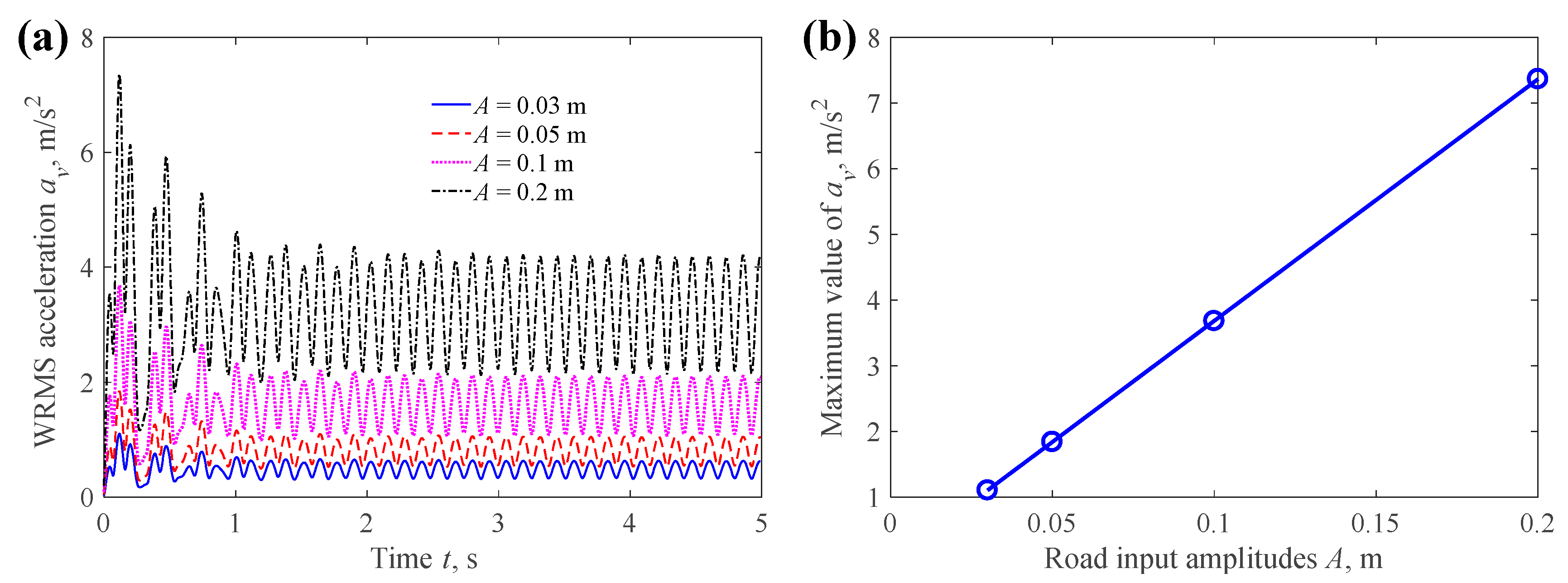
In addition, the WRMS accelerations at various road input amplitudes A are calculated to evaluate vibration comfort. Figure 32 shows that acceleration exhibits a near-linear increase with A. This means that ride comfort decreases as road amplitude increases.

The vertical vibration response of axles for different road input amplitudes is shown in Figure 33. It can be seen that the front and rear axles exhibit similar vibration trends. As the road input amplitude increases, the vertical vibration displacement of both axles also increases.

Therefore, based on the analysis of Figure 31, Figure 32 and Figure 33, pavement input amplitude should be controlled within a safe range to ensure both the safety and comfort of vehicles.

4.3.3. Pavement Input Length

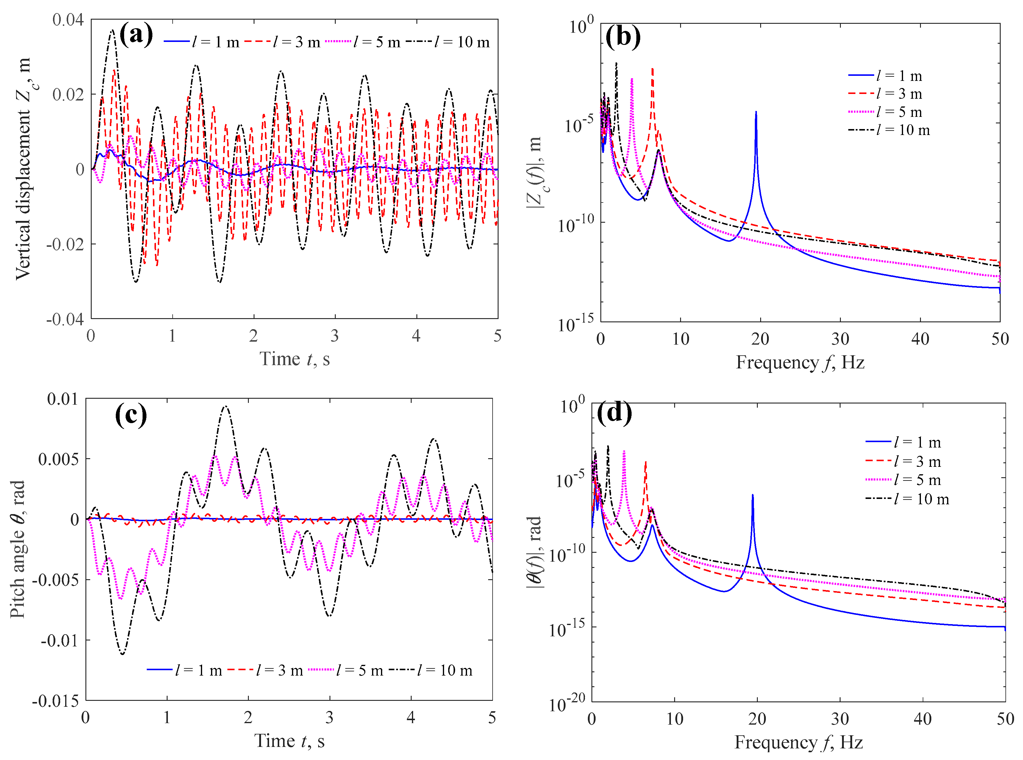
This section analyzes the vehicle’s vibration characteristics under a pavement input amplitude of A = 0.1 m and a speed of v = 70 km/h. Four control tests were conducted, corresponding to different pavement input lengths: l = 1, 3, 5, and 10 m. The fractional orders are set as α = 0.5 and β = 0.5. The MATLAB simulation results are as follows.

The vertical vibration and pitch motion responses of the vehicle body for different road input lengths are shown in Figure 34a,c. The amplitude–frequency curve, obtained by converting time-domain data via the FFT method, is presented in Figure 34b,d. As shown in Figure 34, the initial vibrations exhibit chaotic behavior. The amplitude–frequency response shows that the stable vibration amplitude is smallest at l = 1 m. In contrast, the lengths l = 3 m and l = 10 m exhibit substantially larger amplitudes. According to Figure 34b,d, the excitation frequencies at l = 1 m, 3 m, 5 m, and 10 m are 19.4 Hz, 6.5 Hz, 3.8 Hz, and 1.9 Hz, respectively. In addition, the natural frequencies of the vehicle system are numerically calculated as 0.93 Hz and 7.5 Hz (see Figure 28).

Therefore, it can be concluded that the high vibration amplitude of the vehicle body at l = 3 and 10 m results from the excitation frequencies being close to the system’s natural frequencies.

Moreover, the WRMS accelerations at various l are calculated to evaluate vibration comfort. Figure 35 indicates that the acceleration generally rises with increasing l, with a notable exception at l = 3 m, where an especially large value is observed. The notable amplitude of a_v at l = 3 m is attributed to a resonance phenomenon, resulting from the proximity of the excitation frequency to the natural frequency, combined with a higher excitation frequency (relative to l = 10 m).

It is imperative to avoid the convergence of the vehicle’s natural frequency and excitation frequency during operation. Resonance occurring under such conditions would significantly compromise driving safety and passenger comfort.

5. Conclusions

In this paper, a four-degrees-of-freedom vehicle dynamic model considering fractional damping in suspensions and tires is proposed. The unevenness of the road surface is described by a sinusoidal function. The transfer function method in the Laplace domain is used to obtain the time-domain dynamic responses of the vehicle, including the vertical vibration and pitch motion of the vehicle body, and the front and rear axles’ vertical vibration responses. The transfer function method is verified by comparing with corresponding analytical solutions. The effects of suspension, tire properties, and pavement excitation as well as vehicle speed on car vibration are investigated. Evaluation methods include time-domain vibration response, the amplitude–frequency curve, phase diagrams, the frequency response function matrix, and weighted root mean square acceleration. The main results are listed as follows:

(1) A higher fractional order α shortens the vehicle’s settling time and increases its peak amplitude, at the expense of ride comfort, while having a negligible effect on axle vibration. Similarly, higher suspension stiffness amplifies the stable vibration amplitude and also degrades ride comfort, yet its influence on axle vibration remains minimal. On the other hand, low suspension damping leads to significant initial vibration and an extended settling time, even though it reduces the final amplitude. Although damping has little effect on axle vibration, high damping negatively impacts comfort. Therefore, a trade-off is necessary: to achieve optimal ride comfort, damping should be minimized while still ensuring rapid vibration settling.

(2) Higher tire stiffness reduces the vehicle vibration amplitude. However, the WRMS acceleration exhibits non-monotonic behavior—decreasing initially and then increasing with greater stiffness—suggesting that an optimal value exists for ride comfort. Therefore, optimizing tire stiffness requires balancing both vibration reduction and ride comfort. Additionally, the minimal influence of fractional order β and tire damping on vehicle vibration is due to the significant disparity between the tire’s damping coefficient and its stiffness.

(3) Higher vehicle speed amplifies axle vibration and markedly diminishes ride comfort, underscoring the need to maintain speed within a safe range to ensure both safety and passenger comfort. Similarly, a larger pavement input amplitude exacerbates vehicle vibration and degrades ride quality, necessitating that road excitation levels also be controlled within acceptable limits. These vibrational responses—elevated amplitude and acceleration—arise when excitation frequencies approach the system’s natural frequencies. It is therefore critical to prevent convergence between the vehicle’s natural frequency and external excitation frequencies during operation, as resonance under such conditions would severely jeopardize driving safety and ride comfort.

This study has several limitations, including the use of a sinusoidal road profile, linear springs, and a simplified 2D vehicle model. Future work should extend this research by incorporating random road unevenness, nonlinear springs for both the suspension and tires, and a more sophisticated 3D multi-degree-of-freedom vehicle model. Furthermore, experimental validation is recommended to accurately calibrate the parameters of the fractional damping model.

References

1. Attias, D. The Automobile Revolution; Springer: Cham, Switzerland, 2017. [Google Scholar]
2. Yang, S.; Lu, Y.; Li, S. An overview on vehicle dynamics. Int. J. Dyn. Control 2013, 1, 385–395. [Google Scholar] [CrossRef]
3. Zhou, S.; Song, G.; Sun, M.; Ren, Z. Nonlinear dynamic analysis of a quarter vehicle system with external periodic excitation. Int. J. Nonlin. Mech. 2016, 84, 82–93. [Google Scholar] [CrossRef]
4. Segel, L. An overview of developments in road vehicle dynamics: Past, present and future. In Proceedings of the IMechE Conference on Vehicle Ride and Handling, London, UK, 15–17 November 1993; pp. 1–12. [Google Scholar]
5. Wang, X. Analysis and Research of Vibration Characteristics of Coach. Master’s Thesis, Hefei University of Technology, Hefei, China, 2010. [Google Scholar]
6. Verros, G.; Natsiavas, S.; Papadimitriou, C. Design optimization of quarter-car models with passive and semi-active suspensions under random road excitation. J. Vib. Control 2005, 11, 581–606. [Google Scholar] [CrossRef]
7. Borowiec, M.; Litak, G.; Friswell, M.I. Nonlinear response of an oscillator with a magneto-rheological damper subjected to external forcing. Appl. Mech. Mater. 2006, 5, 277–284. [Google Scholar] [CrossRef]
8. Türkay, S.; Akçay, H. A study of random vibration characteristics of the quarter-car model. J. Sound Vib. 2005, 282, 111–124. [Google Scholar] [CrossRef]
9. Liang, S.; Li, C.; Zhu, Q.; Xiong, Q. The influence of parameters of consecutive speed control humps. J. Vibroeng. 2011, 13, 406–413. [Google Scholar]
10. Paliwal, V.; Dobriyal, R.; Kumar, P.; Manral, A.R. Effect of varying road profile amplitude on the behavior of a nonlinear quarter car model. IOP Conf. Ser. Mater. Sci. Eng. 2021, 1149, 012015. [Google Scholar] [CrossRef]
11. Yang, Z.; Liang, S.; Zhu, Q.; Sun, Y.; Zhan, S. Chaotic Vibration and Comfort Analysis of Nonlinear Half-Vehicle Mode Excited by Consecutive Speed-Control Humps. J. Robot. Mechatron. 2015, 27, 513–519. [Google Scholar] [CrossRef]
12. Zhu, Q.; Ishitobi, M. Chaos and bifurcations in a nonlinear vehicle model. J. Sound Vib. 2004, 275, 1136–1146. [Google Scholar] [CrossRef]
13. Zhu, Q.; Ishitobi, M. Chaotic vibration of a nonlinear full-vehicle model. Int. J. Solids Struct. 2006, 43, 747–759. [Google Scholar] [CrossRef]
14. Cebon, D. Handbook of Vehicle-Road Interaction; Swets & Zeitlinger: Lisse, The Netherlands, 1999. [Google Scholar]
15. Yang, S.; Chen, L.; Li, S. Dynamics of Vehicle-Road Coupled System; Springer: Berlin/Heidelberg, Germany, 2015. [Google Scholar]
16. Li, S.; Yang, S.; Guo, W. Investigation on chaotic motion in hysteretic non-linear suspension system with multi-frequency excitations. Mech. Res. Commun. 2004, 31, 229–236. [Google Scholar] [CrossRef]
17. Dobriyal, R.; Kumar, P.; Jha, N.K.; Paliwal, V.; Gariya, N. Dynamics and optimization of a quarter car model with power law spring. AIP Conf. Proc. 2023, 2521, 020016. [Google Scholar] [CrossRef]
18. Abolfathi, A. Can a nonlinear quasi-zero-stiffness spring improve the ride quality of a vehicle? Veh. Syst. Dyn. 2024, 62, 330–346. [Google Scholar] [CrossRef]
19. Chen, H.; Chen, G.; Meng, Z.; Yang, D. Stochastic bifurcation and dynamic reliability analyses of nonlinear MDOF vehicle system with generalized fractional damping via DPIM. Nonlinear Dynam. 2024, 112, 5291–5316. [Google Scholar] [CrossRef]
20. Mainardi, F. Fractional Calculus and Waves in Linear Viscoelasticity: An Introduction to Mathematical Models; World Scientific: Singapore, 2010. [Google Scholar]
21. Su, X.; Yao, D.; Xu, W. Processing of viscoelastic data via a generalized fractional model. Int. J. Eng. Sci. 2021, 161, 103465. [Google Scholar] [CrossRef]
22. Su, X.; Yao, D.; Xu, W. A new method for formulating linear viscoelastic models. Int. J. Eng. Sci. 2020, 156, 103375. [Google Scholar] [CrossRef]
23. Cai, W.; Wang, P. Fractional modeling of temperature-dependent mechanical behaviors for glassy polymers. Int. J. Mech. Sci. 2022, 232, 107607. [Google Scholar] [CrossRef]
24. Ullah, M.Z.; Mallawi, F.; Baleanu, D.; Alshomrani, A.S. A new fractional study on the chaotic vibration and state-feedback control of a nonlinear suspension system. Chaos Soliton. Fract. 2020, 132, 109530. [Google Scholar] [CrossRef]
25. Nwagoum Tuwa, P.R.; Molla, T.; Noubissie, S.; Kingni, S.T.; Rajagopal, K. Analysis of a quarter car suspension based on a Kelvin–Voigt viscoelastic model with fractional-order derivative. Int. J. Nonlin. Mech. 2021, 137, 103818. [Google Scholar] [CrossRef]
26. Chang, Y.; Zhu, Y.; Li, Y.; Wang, M. Dynamical analysis of a fractional-order nonlinear two-degree-of-freedom vehicle system by incremental harmonic balance method. J. Low Freq. Noise Vib. Act. Control 2024, 43, 706–728. [Google Scholar] [CrossRef]
27. Watanabe, M.; Prasad, A. Fractional delayed feedback for semi-active suspension control of nonlinear jumping quarter car model. Chaos Soliton. Fract. 2025, 199, 116973. [Google Scholar] [CrossRef]
28. Molla, T.; Duraisamy, P.; Rajagopal, K.; Karthikeyan, A.; Boulaaras, S. Exploring nonlinearity in quarter car models with an experimental approach to formulating fractional order form and its dynamic analysis. Sci. Rep. 2024, 14, 12074. [Google Scholar] [CrossRef]
29. Yuvapriya, T.; Lakshmi, P.; Rajendiran, S. Vibration suppression in full car active suspension system using fractional order sliding mode controller. J. Braz. Soc. Mech. Sci. 2018, 40, 217. [Google Scholar] [CrossRef]
30. He, R.; Zhao, B.; Dong, H. Analysis of automobile vibration response based on MATLAB. Auto. Appl. Technol. 2018, 20, 68–70. (In Chinese) [Google Scholar] [CrossRef]
31. Brancik, L. Programs for fast numerical inversion of Laplace transforms in MATLAB language environment. In Proceedings of the 7th Conference MATLAB, Prague, Czech Republic, 21 October 1999; pp. 27–39. [Google Scholar]
32. Gao, S.; Shen, H. Vibration Mechanics; China Railway Press: Beijing, China, 2016. [Google Scholar]
33. Wang, C. Vechicle-Pavement Coupled Vibration Response for Unmanned Driving. Master’s Thesis, Harbin Institute of Technology, Harbin, China, 2022. [Google Scholar]
Figure 1. Fractional replacements for (a) damping elements and (b) Kelvin model, where k is the stiffness coefficient of spring, c is the damping coefficient, and α is the fractional order.
Fractalfract 09 00620 g001
Figure 2. Force-displacement hysteresis curves of fractional Kelvin model with different parameters of (a) k, (b) c and (c) α.
Fractalfract 09 00620 g002
Figure 3. Four-degrees-of-freedom dynamics model of the whole vehicle.
Fractalfract 09 00620 g003
Figure 4. Schematic diagram of sinusoidal pavement excitation model.
Fractalfract 09 00620 g004
Figure 5. Vehicle body force analysis diagram, where I θ ¨ is the inertia moment of the vehicle body corresponding the angular acceleration θ ¨ , m z ¨ c is the inertial force corresponding to vehicle acceleration, and k2 (zc1z1) and h2 Dα(zc1z1) are the elastic force and fractional damping force in the front suspension, respectively. k4 (zc2z2) and h4 Dα(zc2z2) are the elastic force and fractional damping force in the rear suspension, respectively. Parameters zc1 and zc2 are the displacements of the vehicle body in the front and rear suspensions, respectively.
Fractalfract 09 00620 g005
Figure 6. Front axle force analysis, where m 1 z ¨ 1 is the inertial force of the front axle, and k1 (z1z01) and h1 Dβ(z1z01) are the elastic force and fractional damping force in the front tire, respectively.
Fractalfract 09 00620 g006
Figure 7. Rear axle force analysis, where m 2 z ¨ 2 is the inertial force of the rear axle, and k3 (z2z02) and h3 Dβ(z2z02) are the elastic force and fractional damping force in the rear tire, respectively.
Fractalfract 09 00620 g007
Figure 8. Comparison of analytical solutions and numerical results for vibration responses in three degrees of freedom: (a) x1, (b) x2, and (c) x3.
Fractalfract 09 00620 g008
Figure 9. The vibration responses of vehicle the body at different fractional orders α in suspensions: (a) transient and (b) long-term vertical vibrations, (c) transient and (d) long-term pitch motions.
Fractalfract 09 00620 g009
Figure 10. The WRMS acceleration for different values of fractional orders: (a) time-dependent curves and (b) maximum values.
Fractalfract 09 00620 g010
Figure 11. The vertical vibration responses at different fractional orders: (a) front axle and (b) rear axle.
Fractalfract 09 00620 g011
Figure 12. The vibration responses of the vehicle body at different suspension stiffnesses: (a) transient and (b) long-term vertical vibrations, (c) transient and (d) long-term pitch motions.
Fractalfract 09 00620 g012
Figure 13. The phase diagrams of the vehicle body at different suspension stiffnesses: (ad) vertical vibrations, and (eh) pitch motions.
Fractalfract 09 00620 g013
Figure 14. The WRMS acceleration for different values of suspension stiffness: (a) time-dependent curves, and (b) maximum values.
Fractalfract 09 00620 g014
Figure 15. The vertical vibration responses at different suspension stiffnesses: (a) front axle and (b) rear axle.
Fractalfract 09 00620 g015
Figure 16. The vibration responses of the vehicle body at different suspension damping amounts: (a) initial, (b) intermediate, and (c) stable states of vertical vibration, and (d) initial, (e) intermediate, and (f) stable states of pitch motions.
Fractalfract 09 00620 g016
Figure 17. The WRMS acceleration for different values of suspension damping: (a) time-dependent curves, and (b) maximum values.
Fractalfract 09 00620 g017
Figure 18. The phase diagrams of axles at different suspension stiffnesses: (ad) front axle and (eh) rear axle. The red and purple elliptical lines are the reference lines of constant size in Figures (ad) and (eh), respectively, which are used to indicate the relative sizes of the stable vibrational phase diagrams.
Fractalfract 09 00620 g018
Figure 19. The vibration responses of the vehicle body at different fractional orders β in tires: (a) vertical vibration, and (b) pitch motions.
Fractalfract 09 00620 g019
Figure 20. The vertical vibration responses at different fractional orders β in tires: (a) front axle and (b) rear axle.
Fractalfract 09 00620 g020
Figure 21. The vibration responses of the vehicle body at different tire stiffnesses: (a) vertical vibration, and (b) pitch motions.
Fractalfract 09 00620 g021
Figure 22. The phase diagrams of the vehicle body at different tire stiffnesses: (ad) vertical vibration, and (eh) pitch motions. The red and purple elliptical lines are the reference lines of constant size in Figures (ad) and (eh), respectively, which are used to indicate the relative sizes of the stable vibrational phase diagrams.
Fractalfract 09 00620 g022
Figure 23. The WRMS acceleration for different values of tire stiffness: (a) time-dependent curves, and (b) maximum values.
Fractalfract 09 00620 g023
Figure 24. The vertical vibration responses at different tire stiffnesses: (a) front axle and (b) rear axle.
Fractalfract 09 00620 g024
Figure 25. The vibration responses of the vehicle body at different tire damping amounts: (a) vertical vibration, and (b) pitch motions.
Fractalfract 09 00620 g025
Figure 26. The vertical vibration responses at different tire damping amounts: (a) front axle, and (b) rear axle.
Fractalfract 09 00620 g026
Figure 27. Vibration responses of vehicle body at different speeds for (a) vertical vibration, and (c) pitch motion, and corresponding amplitude–frequency curves in (b) and (d), respectively.
Fractalfract 09 00620 g027
Figure 28. FRF amplitude–frequency curve and the natural frequency of the vehicle system.
Fractalfract 09 00620 g028
Figure 29. The WRMS acceleration for different values of vehicle speeds: (a) time-dependent curves, and (b) maximum values.
Fractalfract 09 00620 g029
Figure 30. Vertical vibration responses at different speeds for (a) front axle and (b) rear axle.
Fractalfract 09 00620 g030
Figure 31. Vertical vibration response of the car body with different input amplitudes: (a) vertical vibration, and (b) pitch motion.
Fractalfract 09 00620 g031
Figure 32. The WRMS acceleration for different values of road input amplitudes: (a) time-dependent curves, and (b) maximum values.
Fractalfract 09 00620 g032
Figure 33. Vibration response under different input amplitudes for (a) front axle, and (b) rear axle.
Fractalfract 09 00620 g033
Figure 34. Vibration responses of the vehicle body at different road input lengths for (a) vertical vibration and (c) pitch motion, and corresponding amplitude–frequency curves in (b) and (d), respectively.
Fractalfract 09 00620 g034
Figure 35. The WRMS acceleration for different values of pavement input lengths: (a) time-dependent curves, and (b) maximum values.
Fractalfract 09 00620 g035