Abstract
This paper presents an algorithm for solving the inverse fractional Stefan problem. The considered inverse problem consists of determining the heat transfer coefficient at one of the boundaries of the considered region. The additional information necessary for solving the inverse problem is the set of temperature values in selected points of the region. The fractional derivative with respect to time used in the considered Stefan problem is of the Caputo type. The direct problem was solved by using the alternating phase truncation method adapted to the model with the fractional derivative. To solve the inverse problem, the ant colony algorithm was used. This paper contains an example illustrating the accuracy and stability of the presented algorithm.
1. Introduction
Fractional-order derivatives have found applications in modeling various phenomena, and nowadays, such models using fractional derivatives are commonly studied. One of these is the model of the fractional Stefan problem. It is a generalization of the classic Stefan problem, which is a mathematical model of the phase transition process taking place at a constant temperature. It consists of the simultaneous determination of the state function and the position of the moving interface. This problem is a model for, among other things, the controlled release of a drug from slab matrices [1,2,3], the movement of the shoreline in a sedimentary ocean basin [4,5], and the heat transfer in porous materials [6,7].
The exact solution to the fractional Stefan problem is known only for the most basic case, a one-dimensional case in a semi-infinite region [1,8,9,10] or a two-phase problem, also defined in a semi-infinite region [11,12]. Articles describing approximate methods for solving this kind of problem are not numerous and usually concern one-dimensional and one-phase problems [5,13,14,15]. A numerical method for solving the two-phase problem is presented in [16,17]. A physical interpretation of these kinds of problems was described in paper [18].
So far, the inverse fractional Stefan problem has been considered only in two papers [19,20]. In both papers, a one-phase design problem was considered, which is a problem in which the position of the moving boundary is known. In paper [19], the material parameters were reconstructed for a problem defined in a semi-infinite region. In this paper, solutions of the similarity type were applied. In paper [20], on the other hand, the temperature and heat flux at the boundary of the regions were reconstructed. For the solution to this problem, the homotopy analysis method was used.
This paper, as a first attempt, applies the two-phase fractional Stefan problem to an inverse case. The problem considered in this paper is reconstructing the heat transfer coefficient with the assumption that the temperature measurements at the selected point of the region are known. Using the temperature measurements and the values obtained by solving the direct problem with a set value for the heat transfer coefficient, the functional that represents the error of the approximate solution is constructed. By minimizing this functional, an approximate solution is found. For minimization, the real ant colony optimization algorithm was used. To solve the direct problem, the alternating phase truncation method was adapted.
2. Problem Formulation
The following formulation of the direct problem is the same as that in our previous work [21]. We will consider the one-dimensional two-phase Stefan problem for the solidification process. In the considered region, the two subregions are distinct: , which is taken by the solid phase, and , taken by the liquid phase. The moving interface that separates these phases will be described by the function (see Figure 1).
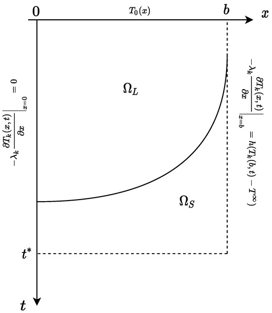
Figure 1.
Scheme of the two-phase problem.
We will use the Caputo fractional derivative of order , , [22]:
where is the gamma function.
The direct problem consists of determining the temperature distributions and in the considered region and the position of the moving interface separating the phases. The temperature distribution in the considered region satisfies the heat transfer equation with a fractional derivative of the Caputo type:
where indicates the specific heat [], is density [], is the scaled thermal conductivity [] [19,23,24,25], is the scaling constant [], and is the thermal conductivity [], where index indicates the solid phase and index the liquid phase. We will assume that the values of the parameters , , , , , and are constant. The scaling constant was introduced (as is standard in the literature) to ensure the consistency of the dimensions of the considered equation.
The initial condition is known:
At the left boundary, the Neumann condition was applied:
and at the right boudary, the Robin boundary condition was applied:
where h [] indicates the heat transfer coefficient, and [] indicates the ambient temperature.
At the boundary s that separates the phases, the Stefan condition with the Caputo derivative was applied:
where L [] is the latent heat of fusion by the unit of mass; and the condition of the temperature continuity is as follows:
where [] refers to the phase-change temperature.
In the inverse problem, the heat transfer coefficient h will be reconstructed. However, the temperature values at a selected point in the area will be known.
3. Solution to the Inverse Problem
The alternating phase truncation method was used to solve the direct problem. The adaptation method for the fractional model was described in a more detailed way in paper [21]. We also refer the reader to this paper for more details on solving the direct problem.
The solution to the inverse Stefan problem consists of repeatedly determining the solution to the direct Stefan problem for fixed values of the heat transfer coefficient h. The values of the temperatures obtained in this way at point at time will be denoted as . Let the approximation error be represented by the following function:
where means the known course of the temperature at point at time . By minimizing the functional (9), the value of the heat transfer coefficient h is being reconstructed. For the minimization of the functional, the real ant colony optimization algorithm (RealACO) [26,27] was used.
This algorithm is inspired by the behavior of ant swarms in nature as they search for a food source. In the mathematical description of the algorithm, the solution (or a point in the search space) is the equivalent to a food source in nature. In the location of the food source, the ants leave a pheromone spot. The ants are tasked with finding the best food source (in other words, solving a problem close to the optimal solution in the search space). During the course of the algorithm, each solution found so far is assigned a probability consistent with the quality of the solution. According to the probability distribution obtained this way in each of the I iterations, M times one solution is selected and then modified. This stage of the algorithm corresponds to the situation in which each of the M ants selects one pheromone spot (or food location) to follow and then moves to another position, where it leaves a new spot. The solutions created in a given iteration are added to the archive, where they are sorted on the basis of their quality. Finally, M of the worst solutions are rejected.
To describe the algorithm, we will use the following notations:
- J—minimized function (or fitness function); n—dimension of the problem;x
- —number of threads; —number of ants in the population;
- I—number of iterations; L—number of pheromone spots; —algorithm tuning parameters.
The steps of the algorithm are as follows:
- Initialization of the algorithm
- Setting the input parameters: .
- Random generation of L initial pheromone spots in the search space. Adding the generated pheromone spots to the initial archive .
- Calculating the values of the fitness function for all the generated solutions (pheromone spots) and sorting the archive elements from the best to the worst solution.
- The iteration process
- 4.
- Assigning the selection probability to each solution using the formulawhere the weight is related to the l-th solution and expressed by
- 5.
- Choosing by ant the l-th solution with the probability .
- 6.
- Transforming the j-th coordinate () of the l-th solution by sampling the neighbourhood using the Gauss probability density functionwhere .
- 7.
- Steps 5–6 are repeated by every ant. In this way, M new solutions (pheromone spots) are created.
- 8.
- The partition of the set of new solutions into groups. Calculating the value of the fitness function for each of the new solutions (parallel computation).
- 9.
- Adding the new solutions to the archive , sorting them by quality and rejecting the M worst solutions.
- 10.
- Steps 3–9 are repeated I times.
4. Example
We will consider the process described by Equations (2)–(8). Let and . We also take the following values: [], [], [], [], [], [], [], [], [], [], and []. All of the calculations presented were performed on the order of the Caputo derivative .
The direct Stefan problem described by Equations (2)–(8) for a given heat transfer coefficient was solved using the alternating phase truncation method, and this way, the temperature course was obtained at point , which was the reference point for comparing the results. From this course, the temperatures were selected to simulate the temperature measurements. From then on, the values obtained in this way were treated as exact ones.
In order to study the impact of the measurement errors on the accuracy of the results obtained and thus test the stability of the algorithm, a frequently applied numerical experiment was used, in which the solution to the direct problem was disturbed by a pseudo-random error. The temperature course obtained in this way was used as the input data for the inverse Stefan problem.
The exact values were obtained using the alternating phase truncation method for a grid size of . The temperature values were measured with point . Measurements were taken every 1, 2, or s. To solve the direct problem in the inverse problem, a grid with a size of was used. The inverse problem was solved for the exact measurements and for the measurements disturbed by the errors by and . The disturbed temperatures are given by
where refers to the measured temperature containing the random error, denotes the exact measured temperature, and is a random variable. The value is randomly selected with a uniform distribution from the interval , where . Figure 2 presents the exact and disturbed input data for the measurements taken every s.
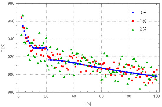
Figure 2.
The exact and disturbed input data presented for the measurements taken every s.
To minimize functional (9), the RealACO algorithm was used with the parameters , , and . The parameters were selected based on previous experiences with the RealACO algorithm and preliminary numerical experiments.
Table 1 presents the results obtained for the data disturbed by errors of , and for the temperature checked every , , and seconds. In every case, a good approximation of the heat transfer coefficient was obtained, as well as the values of the temperatures calculated for the reconstructed coefficient values. For the non-disturbed input data, the best solution was obtained for the temperature measured every s. For the input data disturbed by the error, the best solution was obtained for the temperature checked every s, and in each case, the relative error did not exceed . For measurements disturbed by the error, the best solution was also obtained for the temperature measured every s. The worst solution was received for the temperature checks performed every s, for which the relative error did not exceed .

Table 1.
Results obtained when reconstructing the value of the h coefficient for the data disturbed by , , and (—reconstructed value; —absolute error; —percentage relative error; J—value of the objective function).
Table 2 collects the absolute and relative errors of the temperature reconstruction at the measurement point. In every case, the temperature was well reconstructed. For the exact input data, the absolute maximum error did not exceed K, and the mean error did not exceed K, while the relative errors were % (maximum) and % (mean). For disturbed input data, the worst reconstruction was obtained for the data disturbed by the 2% error. The maximum errors did not exceed K and %, and the mean errors did not exceed K and %.
Table 2.
The errors of the temperature reconstruction at the measurement point (—mean absolute error; —maximum absolute error; —mean relative percentage error; —maximum relative percentage error).
In Figure 3, the reconstructed values of the heat transfer coefficient h are presented depending on the number of iterations for the measurements disturbed, respectively, by and errors for the measurements taken every s.
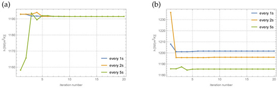
Figure 3.
The reconstructed values of the heat transfer coefficient h for the exact measurement data (a) and data disturbed by the 2% error (b) for different numbers of measurements.
Figure 4 presents a comparison of the exact and reconstructed temperature values at the control point for the measurement data disturbed by errors of and , respectively, for the measurements taken every s. The mean absolute error of reconstruction did not exceed K, while the maximum error did not exceed K. The relative errors, in turn, did not exceed the values of % (mean) and % (maximum).
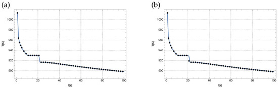
Figure 4.
The temperature course at the measurement point for the measurements disturbed by the 1% error (a) and 2% error (b) (measurements taken every s; solid line—the exact course; dotted line—the reconstructed course).
Figure 5 presents the temperature distribution in the area considered at time s for the exact measurements and for the measurements disturbed by the error for the measurements taken every s. The mean absolute error did not exceed K, while the maximum error did not exceed K. The relative errors, in turn, did not exceed the values % (mean) and % (maximum).
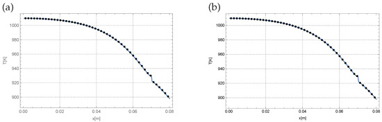
Figure 5.
The temperature distribution at time s for the exact measurements (a) and the measurements disturbed by the 1% error (b) (measurements taken every s; solid line—the exact course; dotted line—the reconstructed course).
5. Conclusions
The subject of this paper was the inverse Stefan problem with a fractional derivative of the Caputo type. In this paper, the value of the heat transfer coefficient was reconstructed while the values of the temperature at the boundary of the region were known. To minimize the functional that represented the reconstruction error, the RealACO algorithm was used, and the solution to the direct problem was obtained using the algorithm of the alternating phase truncation method adapted to the equations with fractional derivatives. The best results were obtained for the input data that consisted of the measurements taken every 1 s. From the presented example, one can conclude that for the proper number of measurements, the algorithm allows us to obtain a good reconstruction as a result.
Calculations were also performed for measurements disturbed by errors of 1% and 2%. In these cases, satisfactory results were also obtained. The errors obtained as a result of reconstructing the heat transfer coefficient did not exceed the values of the errors that the data were disturbed by.
In the future, we plan to work on the inverse Stefan problem with fractional derivatives of different types, where more than one coefficient will be reconstructed.
Author Contributions
Conceptualization: D.S. Methodology: A.C. and D.S. Software: A.C. and R.B. Validation: A.C. and D.S. Investigation: A.C. and D.S. Writing—original draft preparation: A.C. Writing—review and editing: A.C., R.B. and D.S. Funding acquisition: D.S. All authors have read and agreed to the published version of the manuscript.
Funding
This research received no external funding.
Data Availability Statement
The original contributions presented in this study are included in the article. Further inquiries can be directed to the corresponding author.
Acknowledgments
The authors express their sincere thanks to the referees for their time and valuable remarks, which improved this article.
Conflicts of Interest
The authors declare no conflicts of interest.
References
- Liu, J.; Xu, M. An exact solution to the moving boundary problem with fractional anomalous diffusion in drug release devices. ZAMM J. Appl. Math. Mech. 2004, 84, 22–28. [Google Scholar] [CrossRef]
- Yin, C.; Li, X. Anomalous diffusion of drug release from a slab matrix: Fractional diffusion models. Int. J. Pharm. 2011, 418, 78–87. [Google Scholar] [CrossRef]
- Garshasbi, M.; Sanaei, F. A variable time-step method for a space fractional diffusion moving boundary problem: An application to planar drug release devices. Int. J. Numer. Model. 2021, 34, e2852. [Google Scholar] [CrossRef]
- Rajeev; Kushwaha, M.; Kumar, A. An approximate solution to a moving boundary problem with space-time fractional derivative in fluvio-deltaic sedimentation process. Ain Shames Eng. J. 2013, 4, 889–895. [Google Scholar] [CrossRef][Green Version]
- Rajeev; Kushwaha, M. Homotopy perturbation method for a limit case Stefan problem governed by fractional diffusion equation. Appl. Math. Model. 2013, 37, 3589–3599. [Google Scholar] [CrossRef]
- Voller, V. Computations of anomalous phase change. Int. J. Numer. Methods Heat Fluid Flow 2016, 26, 624–638. [Google Scholar] [CrossRef]
- Voller, V. Anomalous heat transfer: Examples, fundamentals, and fractional calculus models. Adv. Heat Transf. 2018, 50, 333–380. [Google Scholar] [CrossRef]
- Liu, J.; Xu, M. Some exact solutions to Stefan problems with fractional differential equations. J. Math. Anal. Appl. 2009, 351, 536–542. [Google Scholar] [CrossRef]
- Roscani, S.; Tarzia, D.; Venturato, L. The similarity method and explicit solutions for the fractional space one-phase Stefan problems. Fract. Calc. Appl. Anal. 2022, 25, 995–1021. [Google Scholar] [CrossRef]
- Ryszewska, K. A space-fractional Stefan problem. Nonlinear Anal. 2020, 199, 112027. [Google Scholar] [CrossRef]
- Roscani, S.; Tarzia, D. Explicit solution for a two-phase fractional Stefan problem with a heat flux condition at the fixed face. Comput. Appl. Math. 2018, 37, 4757–4771. [Google Scholar] [CrossRef]
- Roscani, S.; Caruso, N.; Tarzia, D. Explicit solutions to fractional Stefan-like problems for Caputo and Riemann—Liouville derivatives. Commun. Nonlinear Sci. Numer. Simulat. 2020, 90, 105361. [Google Scholar] [CrossRef]
- Błasik, M.; Klimek, M. Numerical solution of the one phase 1D fractional Stefan problem using the front fixing method. Math. Methods Appl. Sci. 2015, 38, 3214–3228. [Google Scholar] [CrossRef]
- Błasik, M. Numerical scheme for one-phase 1D fractional Stefan problem using the similarity variable technique. J. Appl. Math. Comput. Mech. 2014, 13, 13–21. [Google Scholar] [CrossRef][Green Version]
- Gao, X.; Jiang, X.; Chen, S. The numerical method for the moving boundary problem with space-fractional derivative in drug release devices. Appl. Math. Model. 2015, 39, 2385–2391. [Google Scholar] [CrossRef]
- Błasik, M. A Numerical Method for the Solution of the Two-Phase Fractional Lamé-Clapeyron-Stefan Problem. Mathematics 2020, 8, 2157. [Google Scholar] [CrossRef]
- Rajeev; Singh, A. Homotopy analysis method for a fractional Stefan problem. Nonlinear Sci. Lett. A 2017, 8, 50–59. [Google Scholar]
- Voller, V.; Falcini, F.; Garra, R. Fractional Stefan problems exhibiting lumped and distributed latent-heat memory effects. Phys. Rev. E 2013, 87, 042401. [Google Scholar] [CrossRef]
- Ceretani, A.; Tarzia, D. Determination of two unknown thermal coefficients through an inverse one-phase fractional Stefan problem. Fract. Calc. Appl. Anal. 2017, 20, 399–421. [Google Scholar] [CrossRef]
- Słota, D.; Chmielowska, A.; Brociek, R.; Szczygieł, M. Application of the Homotopy Method for Fractional Inverse Stefan Problem. Energies 2020, 13, 5474. [Google Scholar] [CrossRef]
- Chmielowska, A.; Słota, D. Fractional Stefan Problem Solving by the Alternating Phase Truncation Method. Symmetry 2022, 14, 2287. [Google Scholar] [CrossRef]
- Podlubny, I. Fractional Differential Equations; Academic Press: San Diego, CA, USA, 1999. [Google Scholar] [CrossRef]
- Hristov, J. Approximate solutions to fractional subdiffusion equations. Eur. Phys. J. Spec. Top. 2011, 193, 229–243. [Google Scholar] [CrossRef]
- Brociek, R.; Słota, D.; Król, M.; Matula, G.; Kwaśny, W. Comparison of mathematical models with fractional derivative for the heat conduction inverse problem based on the measurements of temperature in porous aluminum. Int. J. Heat Mass Transf. 2019, 143, 118440. [Google Scholar] [CrossRef]
- Brociek, R.; Wajda, A.; Błasik, M.; Słota, D. An Application of the Homotopy Analysis Method for the Time- or Space-Fractional Heat Equation. Fractal Fract. 2023, 7, 224. [Google Scholar] [CrossRef]
- Socha, K.; Dorigo, M. Ant colony optimization for continuous domains. Eur. J. Oper. Res. 2008, 185, 1155–1173. [Google Scholar] [CrossRef]
- Brociek, R.; Wajda, A.; Słota, D. Comparison of Heuristic Algorithms in Identification of Parameters of Anomalous Diffusion Model Based on Measurements from Sensors. Sensors 2023, 23, 1722. [Google Scholar] [CrossRef]
Disclaimer/Publisher’s Note: The statements, opinions and data contained in all publications are solely those of the individual author(s) and contributor(s) and not of MDPI and/or the editor(s). MDPI and/or the editor(s) disclaim responsibility for any injury to people or property resulting from any ideas, methods, instructions or products referred to in the content. |
© 2025 by the authors. Licensee MDPI, Basel, Switzerland. This article is an open access article distributed under the terms and conditions of the Creative Commons Attribution (CC BY) license (https://creativecommons.org/licenses/by/4.0/).