Finite-Time Cluster Synchronization of Fractional-Order Complex-Valued Neural Networks Based on Memristor with Optimized Control Parameters

Abstract

The finite-time cluster synchronization (FTCS) of fractional-order complex-valued (FOCV) neural network has attracted wide attention. It is inconvenient and difficult to decompose complex-valued neural networks into real parts and imaginary parts. This paper addresses the FTCS of coupled memristive neural networks (CMNNs), which are FOCV systems with a time delay. A controller is designed with a complex-valued sign function to achieve FTCS using a non-decomposition approach, which eliminates the need to separate the complex-valued system into its real and imaginary components. By applying fractional-order stability theory, some conditions are derived for FTCS based on the proposed controller. The settling time, related to the system’s initial values, can be computed using the Mittag–Leffler function. We further investigate the optimization of control parameters by formulating an optimization model, which is solved using particle swarm optimization (PSO) to determine the optimal control parameters. Finally, a numerical example and a comparative experiment are both provided to verify the theoretical results and optimization method.

1. Introduction

Neural networks (NNs) have significant applications across various emerging fields, including multilayer perceptron [1], food quality assessment [2], image recognition [3] and so on [4]. An artificial neural network is a mathematical model that mimics the structure of synaptic connections in the brain to process information. Coupled neural networks (CNNs) enable the interconnection of information between different neurons. With advancements in computers, algorithms, and software, the memristive neural network (MNN) model has gained widespread adoption across diverse domains [5,6,7]. The existence of memristors was confirmed by HP Labs in 2008, and since then, MNNs have been a focal point of research [8,9,10]. MNNs offer memory, adaptability, and high parallel processing capabilities. The features of memristors are close to the characteristics of neuronal synapses [11]. Compared to traditional cellular neural networks, MNNs can construct highly integrated nervous systems that more closely approximate the size and structure of the human brain. Fractional calculus extends integer-order calculus, and models described by fractional differential equations can more accurately simulate real-world systems, particularly viscoelastic models [12]. Complex-valued systems, as an extension of real-valued systems, address certain problems that real-valued systems cannot solve [13,14]. For instance, real-valued systems struggle with symmetry problems and the XOR problem, while a single complex-valued system can handle these issues effectively. In light of these considerations, this paper investigates FOCV-coupled memristive neural networks (FCCMNNs).

Finite-time synchronization (FTS) [15] is notable for its ability to achieve synchronization within a settling time, which has garnered significant attention. Different from asymptotic synchronization, which requires an infinite amount of time, FTS offers practical advantages by reaching synchronization in a predetermined time frame. For effective synchronization within a network, neurons must communicate with one another. In leader-following synchronization scenarios, neurons also need to receive information from a designated leader. Specifically, in the context of cluster synchronization (CS) [16], there may be multiple leaders within each cluster. Consequently, neurons in different clusters must follow the leaders assigned to their respective clusters. Due to its practical implications, CS has attracted considerable interest from researchers [17,18]. This paper addresses the FTCS [19] of FCCMNNs. Neurons within the same cluster can synchronize with their leader’s state, achieving synchronization within a settling time that depends on their initial values.

There are various studies that employ the decomposition method, which converts the complex-valued system into two real-valued parts [13,20,21]. However, in practical applications, decomposing a complex-valued system can be challenging. To address this, the Complex-Valued Sign Function (CVSF) [14] has been introduced, allowing for the direct study of complex-valued systems. For example, if $y=c+d\mathbf{i}$ is a complex number, the CVSF of y is $\left[y\right]=\left[c\right]+\left[d\right]\mathbf{i}$. Additionally, a complex 1-norm [14] is proposed, defined as ${\left|y\right|}_1=\left|c\right|+\left|d\right|\mathbf{i}$. Using the CVSF, a controller is designed to achieve the FTCS of the FCCMNNs without employing the decomposition method. To handle discontinuous terms involving memristors and sign functions, the set-valued map theory [22] and complex-valued Filippov solution [23] are essential. In the study of FTS, it is necessary to calculate the settling time. The Mittag–Leffler function, implemented via the ’mlf’ function in MATLAB, provides a means to compute the settling time.

The proposed controller in this paper is a typical negative feedback controller utilizing the CVSF. In the study of network synchronization, many papers design controllers and provide conditions that control parameters must satisfy, often offering a range for these parameters. However, selecting the optimal control parameters within this broad range is a significant challenge that is frequently overlooked. This paper proposes an optimization model to facilitate the selection of control parameters. The fitness function of the model is constructed according to actual control requirements. The constraints of the model are considered by the theoretical results of FTCS. Due to the complexity of the optimization model, an algorithm based on PSO [24] is proposed to find the optimal solution. This method provides guidance for selecting control parameters, leading to an optimal controller that conserves resources. Typically, research on the synchronization of neural networks (NNs) focuses on synchronization criteria, aiming to reduce control energy through various control methods, such as event-triggered control [25], intermittent control [26], impulsive control [27], adaptive control [28], and sampled control [29]. Among these, feedback control [8] is the most commonly used in practical applications. The proposed optimization method offers guidance for parameter selection in feedback control, contributing to more efficient controller design.

It is natural to incorporate time delay into research, given its significant impact on real systems [30]. The study in [31] addressed the FTCS of FOCV NNs without considering time delay and memristors. Both asymptotic and FTS of coupled NNs, excluding clusters and memristors, were explored in [32], where the focus was on real-valued systems. Additionally, the controller designed in [32] included a time delay, which is not required in this paper. The FTS of FCCMNNs using the decomposition method was investigated in [33]. After decomposition, the research process closely resembles that of real-valued systems. However, there are no prior works that have addressed the FTCS of FCCMNNs using a non-decomposition method. Furthermore, none of the aforementioned studies considered the optimization of control parameters. Therefore, this paper focuses on the FTCS of FCCMNNs, employing a non-decomposition method with optimized control parameters. The major contributions are highlighted below. The difference between this paper and other references is outlined in Table 1.

①

This paper studies the fractional-order CNNs with a time delay, where the network includes memristive elements and complex-valued states, resulting in a model that is not only more complex than those studied in [31,32] but also better suited for simulating real-world scenarios. Unlike the conventional decomposition approach [20,21,34], this study employs a non-decomposition method. Although the decomposition method simplifies theoretical analysis, it often falls short in practical applications. The non-decomposition approach, on the other hand, provides a more realistic representation of complex systems, aligning more closely with real-world dynamics.

②

This paper focuses on FTCS, extending beyond conventional CS [35,36] or FTS [37], which has faster convergence time, and the synchronization time can be calculated in advance. To achieve FTCS, we design a simple controller based on the CVSF and derive synchronization criteria that provide a range of control parameters. The settling time for FTCS can be readily determined through the Mittag–Leffler function. While FTCS has been explored in previous studies [19,31,32], the networks investigated in those works differ significantly from the one considered here. Notably, this is the first study to address FTCS for FOCV-coupled neural networks with memristors using a non-decomposition method.

③

An optimization model solved by PSO is proposed to select the most cost-effective control parameters. This optimization approach guides the selection of control parameters within a broad range that satisfies the synchronization conditions. Although previous studies [31,32] designed similar controllers, they only provided a range for the parameters without specifically focusing on actual control requirement.

Table 1. The difference between this paper and others in the literature.

Item	[19]	[32]	[20]	[31]	[34]	[21]	[37]	This Paper
Fractional-order		✓		✓		✓	✓	✓
Complex-valued			✓	✓	✓	✓	✓	✓
Memristor			✓		✓	✓		✓
FTS	✓	✓	✓		✓		✓	✓
CS	✓	✓		✓				✓
Non-decomposition				✓			✓	✓
Parameter optimization								✓

Table 1. The difference between this paper and others in the literature.

Item	[19]	[32]	[20]	[31]	[34]	[21]	[37]	This Paper
Fractional-order		✓		✓		✓	✓	✓
Complex-valued			✓	✓	✓	✓	✓	✓
Memristor			✓		✓	✓		✓
FTS	✓	✓	✓		✓		✓	✓
CS	✓	✓		✓				✓
Non-decomposition				✓			✓	✓
Parameter optimization								✓

The remainder of this paper is structured as follows: Section 2 outlines the essential definitions and lemmas, as well as the model of FCCMNNs and the foundational assumptions. Section 3 introduces the designed controller and provides the theorem for achieving FTCS. Section 4 is dedicated to the optimization of control parameters. Section 5 illustrates the effectiveness of the proposed methods through two simulations. Finally, Section 6 provides the conclusions.

Notations. 

$\mathbb{R},{\mathbb{R}}^n,{\mathbb{R}}^{n\times n}$ represent the set of real numbers, n-dimensional real vectors and $n\times n$ real matrices, respectively. $N^{+}$ denotes the set of positive integers. $\mathbb{C},{\mathbb{C}}^n,{\mathbb{C}}^{n\times n}$ represent the set of complex numbers, n-dimensional complex vectors and $n\times n$ complex matrices. If $y\in \mathbb{C}$, $y=y^R+y^I\mathbf{i}$. $y^R$ and $y^I$ means real and imaginary parts of y, $\mathbf{i}$ is the imaginary unit. ${\left|y\right|}_1=|y^R|+|y^I|$. $\left[y\right]=\left[y^R\right]+\left[y^I\right]\mathbf{i}$, and $[·]$ represents the sign function. If $Y\in {\mathbb{C}}^n$, $Y=(y_1,y_2,\cdots ,y_n)$. $Y^H$ is the conjugate transpose of $Y.$ $Y^T$ is the transpose of $Y.$ ${\left|Y\right|}_1={\sum }_{i=1}^n\left(\right|y_i^R|+|y_i^I\left|\right)$. $\left[Y\right]=(\left[y_1\right],\left[y_2\right],\cdots ,\left[y_n\right])$. $\Theta \in {\mathbb{R}}^{n\times n}>0$ means that $\Theta$ is a positive definite matrix. ${\lambda }_{min}(\Theta )$ is the minimum eigenvalue of $\Theta$. $diag(\cdots )$ denotes a diagonal matrix. The notation ⊗ is the Kronecker product operator. $I_N$ is an N-dimensional identity matrix. ${\mathbf{1}}_N$ is an N-dimensional full one vectors.

2. Preliminaries and Model Description

2.1. Preliminaries

Definition 1

([14]). The sign function of the complex vector $x\left(t\right)={\left(x_1\left(t\right),x_2\left(t\right),\cdots ,x_n\left(t\right)\right)}^T$ is defined by $\left[x\left(t\right)\right]={\left(\left[x_1^R\left(t\right)\right]+\left[x_1^I\left(t\right)\right]\mathbf{i},\left[x_2^R\left(t\right)\right]+\left[x_2^I\left(t\right)\right]\mathbf{i},\cdots ,\left[x_n^R\left(t\right)\right]+\left[x_n^I\left(t\right)\right]\mathbf{i}\right)}^T$, where $[·]=sign(·)$ and $sign(·)$ is the sign function. Obviously, $\left[x^H\left(t\right)\right]={\left[x\left(t\right)\right]}^H$.

Definition 2

([38]). When fractional order $\alpha \in (0,1)$, the Caputo derivative with function $\omega \left(s\right)$ is defined as:

$$D_{t_0,t}^{\alpha }\omega \left(s\right)={\displaystyle \frac{1}{\Gamma (1-\alpha )}}{\int }_{t_0}^t{(s-\tau )}^{-\alpha }{\omega }^{\prime }\left(\tau \right)d\tau ,$$

(1)

where $t\ge t_0$, and $\Gamma (·)$ is the Gamma function that $\Gamma \left(\alpha \right)={\int }_0^{\infty }{t}^{\alpha -1}{e}^{-t}dt.$

Definition 3

([38]). The two-parameter Mittag–Leffler function is defined by the series expansion

$$E_{p,q}\left(x\right)=\sum _{j=0}^{+\infty }{\displaystyle \frac{x^j}{\Gamma (pj+q)}},$$

(2)

where $p,q>0,x\in \mathbb{C}$. As $q=1,$ the one-parameter Mittag–Leffler function is

$$E_p\left(x\right)=E_{p,1}\left(x\right)=\sum _{j=0}^{+\infty }{\displaystyle \frac{x^j}{\Gamma (pj+1)}},$$

(3)

where $\Gamma (·)$ is the same Gamma function with Definition 2.

For any $x\left(t\right)\in {\mathbb{C}}^n$, the convex hull of $\left[x_j\left(t\right)\right](j=1,2,\cdots ,n)$ is defined as [14]:

$$\begin{array}{cc}\hfill \overline{co}\left(\left[x_j\left(t\right)\right]\right)& =\left\{\begin{array}{cc}\{1+\mathbf{i}\},\hfill & x_j^R\left(t\right)>0,x_j^I\left(t\right)>0,\hfill \\ 1+\overline{co}\{-1,1\}\mathbf{i},\hfill & x_j^R\left(t\right)>0,x_j^I\left(t\right)=0,\hfill \\ \{1-\mathbf{i}\},\hfill & x_j^R\left(t\right)>0,x_j^I\left(t\right)<0,\hfill \\ \overline{co}\{-1,1\}+\mathbf{i},\hfill & x_j^R\left(t\right)=0,x_j^I\left(t\right)>0,\hfill \\ \overline{co}\{-1,1\}+\overline{co}\{-1,1\}\mathbf{i},\hfill & x_j^R\left(t\right)=0,x_j^I\left(t\right)=0,\hfill \\ \overline{co}\{-1,1\}-\mathbf{i},\hfill & x_j^R\left(t\right)=0,x_j^I\left(t\right)<0,\hfill \\ \{-1+\mathbf{i}\},\hfill & x_j^R\left(t\right)<0,x_j^I\left(t\right)>0,\hfill \\ -1+\overline{co}\{-1,1\}\mathbf{i},\hfill & x_j^R\left(t\right)<0,x_j^I\left(t\right)=0,\hfill \\ \{-1-\mathbf{i}\},\hfill & x_j^R\left(t\right)<0,x_j^I\left(t\right)<0.\hfill \end{array}\right.\hfill \end{array}$$

(4)

Lemma 1.

For column vector $\chi \left(t\right):[t_0,+\infty )\to {\mathbb{C}}^n$, there are some properties.

①

[31] $2\left[{\chi }^H\left(t\right)\right]\left[\chi \left(t\right)\right]=\left[{\chi }^H\left(t\right)\right]\omega \left(t\right)+{\omega }^H\left(t\right)\left[\chi \left(t\right)\right]$, where $\omega \left(t\right)={({\omega }_1\left(t\right),{\omega }_2\left(t\right),\cdots ,{\omega }_n\left(t\right))}^T\in \overline{co}\left(\left[\chi \left(t\right)\right]\right)$.

②

[14] ${\chi }_p^H\left(t\right)+{\chi }_p\left(t\right)=2{\chi }_p^R\left(t\right)\le 2{\left|{\chi }_p\left(t\right)\right|}_1,p=1,2,\cdots ,n$.

③

${2\left|\chi \left(t\right)\right|}_1=\left[{\chi }^H\left(t\right)\right]\chi \left(t\right)+{\chi }^H\left(t\right)\left[\chi \left(t\right)\right]$.

④

${\left|\left[\chi \left(t\right)\right]\right|}_1=\left[{\chi }^H\left(t\right)\right]\left[\chi \left(t\right)\right]$.

Proof. 

Based on the definition of ${\left|\chi \left(t\right)\right|}_1,\left[\chi \left(t\right)\right]$ and the Lemma 3 in [14], one has

③

$$\begin{array}{cc}\hfill {2\left|\chi \left(t\right)\right|}_1& =2\sum _{p=1}^n{\left|{\chi }_p\left(t\right)\right|}_1=\sum _{p=1}^n\left(\left[\overline{{\chi }_p\left(t\right)}\right]{\chi }_p\left(t\right)+\overline{{\chi }_p\left(t\right)}\left[{\chi }_p\left(t\right)\right]\right)=\left[{\chi }^H\left(t\right)\right]\chi \left(t\right)+{\chi }^H\left(t\right)\left[\chi \left(t\right)\right].\hfill \end{array}$$

④

$$\begin{array}{cc}\hfill {\left|\left[\chi \left(t\right)\right]\right|}_1& =\sum _{p=1}^n{\left|\left[{\chi }_p\left(t\right)\right]\right|}_1=\sum _{p=1}^n\left[\overline{{\chi }_p\left(t\right)}\right]\left[{\chi }_p\left(t\right)\right]=\left[{\chi }^H\left(t\right)\right]\left[\chi \left(t\right)\right].\hfill \end{array}$$

□

Lemma 2

([37]). If there is a continuous and analytic function $\chi \left(t\right)={\left({\chi }_1\left(t\right),{\chi }_2\left(t\right),\cdots ,{\chi }_n\left(t\right)\right)}^T\in {\mathbb{C}}^n$, then for $t\in [t_0,+\infty ),\alpha \in (0,1)$, one has:

$$\begin{array}{cc}\hfill & D_{t_0,t}^{\alpha }\left(\left[{\chi }^H\left(t\right)\right]\chi \left(t\right)+{\chi }^H\left(t\right)\left[\chi \left(t\right)\right]\right)\le \left[{\chi }^H\left(t\right)\right]D_{t_0,t}^{\alpha }\chi \left(t\right)+D_{t_0,t}^{\alpha }{\chi }^H\left(t\right)\left[\chi \left(t\right)\right].\hfill \end{array}$$

(5)

Lemma 3.

If there is a continuous and differentiable function $v\left(t\right)>0$, $t\in [t_0,+\infty )$, $v\left(t_0\right)>0$, ${\kappa }_1,{\kappa }_2>0$, $\alpha \in (0,1]$, then for $D_{t_0,t}^{\alpha }v\left(t\right)\le -{\kappa }_{1}v\left(t\right)-{\kappa }_2,$ one has

①

[32] $v\left(t\right)\le \left(v\left(t_0\right)+{\displaystyle \frac{{\kappa }_2}{{\kappa }_1}}\right)E_{\alpha }\left(-{\kappa }_1{(t-t_0)}^{\alpha }\right)-{\displaystyle \frac{{\kappa }_2}{{\kappa }_1}}$.

②

There exists $t^{\ast }>t_0$ such that ${lim}_{t\to t^{\ast }}v\left(t\right)\to 0$, when $t\ge t^{\ast }$, $v\left(t\right)\equiv 0$. $t^{\ast }=t_0+{\left(-{\displaystyle \frac{\varpi }{{\kappa }_1}}\right)}^{{\displaystyle \frac{1}{\alpha }}}$, where $\varpi =max\left\{y|E_{\alpha }\left(y\right)={\displaystyle \frac{{\kappa }_2}{{\kappa }_{1}v\left(t_0\right)+{\kappa }_2}}\right\}$.

Proof. 

As demonstrated in [31], let $\Sigma \left(t\right)=\left(v\left(t_0\right)+{\displaystyle \frac{{\kappa }_2}{{\kappa }_1}}\right)E_{\alpha }\left(-{\kappa }_1{(t-t_0)}^{\alpha }\right)-{\displaystyle \frac{{\kappa }_2}{{\kappa }_1}}$. Since ${\kappa }_1>0$ and $\alpha \in (0,1]$, it is clear that $E_{\alpha }\left(-{\kappa }_1{(t-t_0)}^{\alpha }\right)$ is non-increasing. Firstly, the existence of $t^{\ast }$ needs to be verified. Obviously, $E_{\alpha }\left(0\right)=1$ and ${lim}_{t\to +\infty }{E}_{\alpha }(-t)=0$, then $\Sigma \left(t_0\right)=v\left(t_0\right)>0$, ${lim}_{t\to \infty }\Sigma \left(t\right)=-{\displaystyle \frac{{\kappa }_2}{{\kappa }_1}}<0$. Consequently, there is $t^{\ast }>t_0$ such that $\Sigma \left(t^{\ast }\right)=0$. That is to say $E_{\alpha }\left(-{\kappa }_1{(t^{\ast }-t_0)}^{\alpha }\right)={\displaystyle \frac{{\kappa }_2}{{\kappa }_{1}v\left(t_0\right)+{\kappa }_2}}$. In addition, $t^{\ast }=t_0+{\left(-{\displaystyle \frac{\varpi }{{\kappa }_1}}\right)}^{{\displaystyle \frac{1}{\alpha }}}$, where $\varpi =max\left\{y|E_{\alpha }\left(y\right)={\displaystyle \frac{{\kappa }_2}{{\kappa }_{1}v\left(t_0\right)+{\kappa }_2}}\right\}<0$. Secondly, it is proved by contradiction that $v\left(t\right)\equiv 0(t\ge t^{\ast })$. If $v\left(t\right)\equiv 0(t\ge t^{\ast })$ is not true, then $\exists t^{\prime }>t^{\ast }$ such that $v\left(t^{\prime }\right)>0$. However, $v\left(t^{\prime }\right)\le \Sigma \left(t^{\prime }\right)=\left(v\left(t_0\right)+{\displaystyle \frac{{\kappa }_2}{{\kappa }_1}}\right)E_{\alpha }\left(-{\kappa }_1{(t^{\prime }-t_0)}^{\alpha }\right)-{\displaystyle \frac{{\kappa }_2}{{\kappa }_1}}\le \left(v\left(t_0\right)+{\displaystyle \frac{{\kappa }_2}{{\kappa }_1}}\right)E_{\alpha }\left(-{\kappa }_1{(t^{\ast }-t_0)}^{\alpha }\right)-{\displaystyle \frac{{\kappa }_2}{{\kappa }_1}}=0$, which is a contradiction with $v\left(t^{\prime }\right)>0$. Consequently, there exists $t^{\ast }>t_0$ such that ${lim}_{t\to t^{\ast }}v\left(t\right)\to 0$, when $t\ge t^{\ast }$, $v\left(t\right)\equiv 0$. □

2.2. Model Description

An FCCMNN with a time delay is considered as follows:

$$\begin{array}{cc}\hfill D_{t_0,t}^{\alpha }{z}_i\left(t\right)=& -C{z}_i\left(t\right)+A\left(z_i\left(t\right)\right)f\left(z_i\left(t\right)\right)+B\left(z_i\left(t\right)\right)f\left(z_i(t-\tau )\right)+\sigma \sum _{j=1}^N{g}_{ij}\Gamma z_j\left(t\right)+I\left(t\right)+u_i\left(t\right),\hfill \end{array}$$

(6)

where $\alpha \in (0,1)$, $i,j=1,2,\cdots ,N$. $z_i(t-\tau )={\left(z_{i1}(t-\tau ),z_{i2}(t-\tau ),\cdots ,z_{in}(t-\tau )\right)}^T\in {\mathbb{C}}^n$ and $z_i\left(t\right)={\left(z_{i1}\left(t\right),z_{i2}\left(t\right),\cdots ,z_{in}\left(t\right)\right)}^T\in {\mathbb{C}}^n$ are the state of ith neuron with and without the time delay, $0<\tau \le {\tau }_{max}$. $C=diag(c_1,\cdots ,c_n)\in {\mathbb{C}}^{n\times n}$. $f(\ast ):{\mathbb{C}}^n\to {\mathbb{C}}^n$ represents the activation function. $\sigma >0$ is the coupled strength. $G={\left(g_{ij}\right)}_{N\times N}$ and $g_{ij}\in \mathbb{R}$, $g_{ij}\ne 0$ means that the neuron i can receive the information from the neuron j. Otherwise, there is no link. Define $g_{ii}=-{\sum }_{j=1,i\ne j}^N{g}_{ij}$, which is equivalent to ${\sum }_{j=1}^N{g}_{ij}=0$. $\Gamma =diag\{{\gamma }_1,{\gamma }_2,\cdots ,{\gamma }_n\}\in {\mathbb{R}}^{n\times n}$ is an inner matrix and $\Gamma >0$. $I\left(t\right)\in {\mathbb{C}}^n$ is an external input. $u_i\left(t\right)$ is the controller that needs to be designed. $A\left(z_i\left(t\right)\right)={\left(a_{pq}\left(z_{ip}\left(t\right)\right)\right)}_{n\times n}$, $B\left(z_i\left(t\right)\right)={\left(b_{pq}\left(z_{ip}\left(t\right)\right)\right)}_{n\times n}$, and $A\left(z_i\left(t\right)\right),B\left(z_i\left(t\right)\right)\in {\mathbb{C}}^{n\times n}$. Based on the characteristics of memristors, $a_{pq}\left(z_{ip}\left(t\right)\right)$ and $b_{pq}\left(z_{ip}\left(t\right)\right)$ are given as follows:

$$a_{pq}\left(z_{ip}\left(t\right)\right)=\left\{\begin{array}{ccc}\hfill {\acute{a}}_{pq},& \hfill & \hfill |z_{ip}{\left(t\right)|}_1\le I,\\ \hfill {\stackrel{‵}{a}}_{pq},& \hfill & \hfill |z_{ip}{\left(t\right)|}_1>I,\end{array}\right.b_{pq}\left(z_{ip}\left(t\right)\right)=\left\{\begin{array}{ccc}\hfill {\acute{b}}_{pq},& \hfill & \hfill |z_{ip}{\left(t\right)|}_1\le I,\\ \hfill {\stackrel{‵}{b}}_{pq},& \hfill & \hfill |z_{ip}{\left(t\right)|}_1>I,\end{array}\right.$$

(7)

where $I>0$ represents the switching jump, ${\acute{a}}_{pq},{\stackrel{‵}{a}}_{pq},{\acute{b}}_{pq}$ and ${\stackrel{‵}{b}}_{pq}$ are all known complex numbers, $p,q=1,2,\cdots ,n$. The initial value of network (6) is that $z_i\left(w\right)={\psi }_i\left(w\right),w\in [t_0-\tau ,t_0],i=1,2,\cdots ,N$.

The leaders of the network (6) is stated as follows:

$$\begin{array}{cc}\hfill D_{t_0,t}^{\alpha }{s}_l\left(t\right)=& -C{s}_l\left(t\right)+A\left(s_l\left(t\right)\right)f\left(s_l\left(t\right)\right)+B\left(s_l\left(t\right)\right)f\left(s_l(t-\tau )\right)+I\left(t\right),\hfill \end{array}$$

(8)

where $s_l\left(t\right)={\left(s_{l1}\left(t\right),s_{l2}\left(t\right),\cdots ,s_{ln}\left(t\right)\right)}^T\in {\mathbb{C}}^n$ is the leader of the lth cluster. The initial value of network (8) is that $s_l\left(w\right)={\varphi }_l\left(w\right),w\in [t_0-\tau ,t_0],l=1,2,\cdots ,m,m\in {\mathbb{N}}^{+}$. The definitions of $C,A(·),B(·),f(·),I\left(t\right)$ are same with Equation (6).

Suppose that all neurons in network (6) are divided into m clusters, with neurons within the same cluster following the same leader. For example,

$$\begin{array}{cc}\hfill & z_{n_0+1}\left(t\right),\cdots ,z_{n_0+n_1}\left(t\right)⇝s_1\left(t\right),\hfill \\ \hfill & z_{n_0+n_1+1}\left(t\right),\cdots ,z_{n_0+n_1+n_2}\left(t\right)⇝s_2\left(t\right),\cdots ,\hfill \\ \hfill & z_{n_0+n_1+\cdots +n_{m-1}+1}\left(t\right),\cdots ,z_{n_0+n_1+n_2+\cdots +n_m}\left(t\right)⇝s_m\left(t\right),\hfill \end{array}$$

(9)

where $n_l$ is the number of neurons in the lth cluster, $l=1,2,\cdots ,m$, $n_0=0,n_0+n_1+n_2+\cdots +n_m=N$. Define ${\Lambda }_l=\{n_0+n_1+\cdots +n_{l-1}+1,\cdots ,n_0+n_1+\cdots +n_l\}.$

According to the set-valued map theory and complex-valued Filippov solution [34], the networks (6) and (8) can be rewritten to Equations (10) and (11).

$$\begin{array}{cc}\hfill D_{t_0,t}^{\alpha }{z}_i\left(t\right)=& -C{z}_i\left(t\right)+\tilde{A}\left(z_i\left(t\right)\right)f\left(z_i\left(t\right)\right)+\tilde{B}\left(z_i\left(t\right)\right)f\left(z_i(t-\tau )\right)+\sigma \sum _{j=1}^N{g}_{ij}\Gamma z_j\left(t\right)+I\left(t\right)+u_i\left(t\right),\hfill \end{array}$$

(10)

$$\begin{array}{cc}\hfill D_{t_0,t}^{\alpha }{s}_l\left(t\right)=& -C{s}_l\left(t\right)+\tilde{A}\left(s_l\left(t\right)\right)f\left(s_l\left(t\right)\right)+\tilde{B}\left(s_l\left(t\right)\right)f\left(s_l(t-\tau )\right)+I\left(t\right).\hfill \end{array}$$

(11)

where $\tilde{A}\left(z_i\left(t\right)\right)={\left(\widetilde{a_{pq}}\left(z_{ip}\left(t\right)\right)\right)}_{n\times n},\tilde{B}\left(z_i\left(t\right)\right)={\left(\widetilde{b_{pq}}\left(z_{ip}\left(t\right)\right)\right)}_{n\times n},\widetilde{a_{pq}}\left(z_{ip}\left(t\right)\right)\in \overline{co}\left[a_{pq}\left(z_{ip}\left(t\right)\right)\right],\widetilde{b_{pq}}\left(z_{ip}\left(t\right)\right)\in \overline{co}\left[b_{pq}\left(z_{ip}\left(t\right)\right)\right]$. $\overline{co}[·]$ is a convex hull. Similarly, $\tilde{A}\left(s_l\left(t\right)\right)={\left(\widetilde{a_{pq}}\left(s_{lp}\left(t\right)\right)\right)}_{n\times n},\tilde{B}\left(s_l\left(t\right)\right)={\left(\widetilde{b_{pq}}\left(s_{lp}\left(t\right)\right)\right)}_{n\times n}$. It is worth noting that $\widetilde{a_{pq}}\left(s_{lp}\left(t\right)\right)\ne \widetilde{a_{pq}}\left(z_{ip}\left(t\right)\right)$, and $\widetilde{b_{pq}}\left(s_{lp}\left(t\right)\right)\ne \widetilde{b_{pq}}\left(z_{ip}\left(t\right)\right),p,q=1,2,\cdots ,n$.

For convenience, there are some assumptions and propositions.

Assumption 1.

$G={\left(g_{ij}\right)}_{N\times N}$ is the adjacent matrix of network (6),

$$G=\left(\begin{array}{cccc}{G}_{11}& G_{12}& \cdots & G_{1m}\\ G_{21}& G_{22}& \cdots & G_{2m}\\ ⋮& ⋮& \ddots & ⋮\\ G_{m1}& G_{m2}& \cdots & G_{mm}\end{array}\right),$$

(12)

where $G_{ll}\in {\mathbb{R}}^{n_l\times n_l}$, $G_{kl}\in {\mathbb{R}}^{n_k\times n_l}(k\ne l)$. Suppose that $G_{ll}$ and $G_{kl}$ are both zero row-sum matrices, $k,l=1,2,\cdots ,m$. Obviously, G is a zero row-sum matrix.

Assumption 2.

① For $a,b\in \mathbb{C}$, there exists $L>0$, such that the activation functions $f\left(\right)$ satisfies ${|f\left(a\right)-f\left(b\right)|}_1\le L{|a-b|}_1$. ② There exists $F>0$, such that ${\left|f\left(c\right)\right|}_1\le F$ for $\forall c\in \mathbb{C}$.

Proposition 1.

Given Assumptions 1 and 2, the following inequalities can be derived:

①

$$\begin{array}{cc}& |\widetilde{a_{pq}}\left(z_{ip}\left(t\right)\right)f_q\left(z_{iq}\left(t\right)\right)-\widetilde{a_{pq}}\left(s_{lp}\left(t\right)\right)f_q\left(s_{lq}\left(t\right)\right){|}_1\le {\overline{a}}_{pq}L{\left|e_{iq}\left(t\right)\right|}_1+{\check{a}}_{pq}F;\hfill \end{array}$$

②

$$\begin{array}{cc}& |\widetilde{b_{pq}}\left(z_{ip}\left(t\right)\right)f_q\left(z_{iq}(t-\tau )\right)-\widetilde{b_{pq}}\left(s_{lp}\left(t\right)\right)f_q\left(s_{lq}(t-\tau )\right){|}_1\le 2{\overline{b}}_{pq}F;\hfill \end{array}$$

where ${\overline{a}}_{pq}=max\left\{\right|{\acute{a}}_{pq}{|}_1,|{\stackrel{‵}{a}}_{pq}{|}_1\}$, ${\overline{b}}_{pq}=max\left\{\right|{\acute{b}}_{pq}{|}_1,|{\stackrel{‵}{b}}_{pq}{|}_1\}$, ${\check{a}}_{pq}={|{\acute{a}}_{pq}-{\stackrel{‵}{a}}_{pq}|}_1$, $i=1,2,\cdots ,N$, $l=1,2,\cdots ,m$, $p,q=1,2,\cdots ,n$.

Proof. 

①

$$\begin{array}{cc}& |\widetilde{a_{pq}}\left(z_{ip}\left(t\right)\right)f_q\left(z_{iq}\left(t\right)\right)-\widetilde{a_{pq}}\left(s_{lp}\left(t\right)\right)f_q\left(s_{lq}\left(t\right)\right){|}_1\hfill \\ \hfill =& |\widetilde{a_{pq}}\left(z_{ip}\left(t\right)\right)f_q\left(z_{iq}\left(t\right)\right)-\widetilde{a_{pq}}\left(z_{ip}\left(t\right)\right)f_q\left(s_{lq}\left(t\right)\right)+\widetilde{a_{pq}}\left(z_{ip}\left(t\right)\right)f_q\left(s_{lq}\left(t\right)\right)-\widetilde{a_{pq}}\left(s_{lp}\left(t\right)\right)f_q\left(s_{lq}\left(t\right)\right){|}_1\hfill \\ \hfill =& |\widetilde{a_{pq}}\left(z_{ip}\left(t\right)\right)\left(f_q\left(z_{iq}\left(t\right)\right)-f_q\left(s_{lq}\left(t\right)\right)\right)+\left(\widetilde{a_{pq}}\left(z_{ip}\left(t\right)\right)-\widetilde{a_{pq}}\left(s_{lp}\left(t\right)\right)\right)f_q\left(s_{lq}\left(t\right)\right){|}_1\hfill \\ \hfill \le & {\overline{a}}_{pq}L{\left|e_{iq}\left(t\right)\right|}_1+{\check{a}}_{pq}F;\hfill \end{array}$$

②

$$\begin{array}{cc}& |\widetilde{b_{pq}}\left(z_{ip}\left(t\right)\right)f_q\left(z_{iq}(t-\tau )\right)-\widetilde{b_{pq}}\left(s_{lp}\left(t\right)\right)f_q\left(s_{lq}(t-\tau )\right){|}_1\hfill \\ \hfill \le & \left|\widetilde{b_{pq}}\left(z_{ip}\left(t\right)\right){|}_1\right|f_q\left(z_{iq}(t-\tau )\right){|}_1+\left|\widetilde{b_{pq}}\left(s_{lp}\left(t\right)\right){|}_1\right|f_q\left(s_{lq}(t-\tau )\right){|}_1\hfill \\ \hfill \le & 2{\overline{b}}_{pq}F.\hfill \end{array}$$

□

Define the synchronization error: $e_i\left(t\right)=z_i\left(t\right)-s_l\left(t\right),i\in \forall {\Lambda }_l,l=1,2,\cdots ,m$. Based on Assumption 1 that G is a zero row-sum matrix, controlled error network can be described as follows:

$$\begin{array}{cc}\hfill D_{t_0,t}^{\alpha }{e}_i\left(t\right)=& -C{e}_i\left(t\right)+\tilde{A}\left(e_i\left(t\right)\right)\tilde{f}\left(e_i\left(t\right)\right)+\tilde{B}\left(e_i\left(t\right)\right)\tilde{f}\left(e_i(t-\tau )\right)+\sigma \sum _{j=1}^N{g}_{ij}\Gamma e_j\left(t\right)+u_i\left(t\right),\hfill \end{array}$$

(13)

where $\tilde{A}\left(e_i\left(t\right)\right)\tilde{f}\left(e_i\left(t\right)\right)=\tilde{A}\left(z_i\left(t\right)\right)f\left(z_i\left(t\right)\right)-\tilde{A}\left(s_l\left(t\right)\right)f\left(s_l\left(t\right)\right)$, $\tilde{B}\left(e_i\left(t\right)\right)\tilde{f}\left(e_i(t-\tau )\right)=\tilde{B}\left(z_i\left(t\right)\right)f\left(z_i(t-\tau )\right)-\tilde{B}\left(s_l\left(t\right)\right)f\left(s_l(t-\tau )\right)$.

Definition 4

([31]). The networks (6) and (8) achieve the FTCS, if there exists the settling time $t^{\ast }>t_0$ and satisfies:

①

${\overline{lim}}_{t\to \infty }{|s_k\left(t\right)-s_l\left(t\right)|}_1>0,k\ne l,k,l=1,2,\cdots ,m$;

②

${lim}_{t\to t^{\ast }}{|x_i\left(t\right)-s_l\left(t\right)|}_1=0,i\in {\Lambda }_l,l=1,2,\cdots ,m;$

③

$|x_i\left(t\right)-s_l{\left(t\right)|}_1\equiv 0,t\ge t^{\ast },i\in {\Lambda }_l,l=1,2,\cdots ,m$.

3. Main Results

To achieve the FTCS of the networks (6) and (8), a novel controller with CVSF is designed.

$$u_i\left(t\right)=-k_i^1{e}_i\left(t\right)-k^2\left[e_i\left(t\right)\right],$$

(14)

where $k_i^1>0,k^2=diag(k_1^2,k_2^2,\cdots ,k_n^2)\in {\mathbb{R}}^{n\times n}>0$ is a diagonal matrix. Based on Equation (14), the error network (13) can be written to

$$\begin{array}{cc}\hfill D_{t_0,t}^{\alpha }{e}_i\left(t\right)=& -C{e}_i\left(t\right)+\tilde{A}\left(e_i\left(t\right)\right)\tilde{f}\left(e_i\left(t\right)\right)+\tilde{B}\left(e_i\left(t\right)\right)\tilde{f}\left(e_i(t-\tau )\right)+\sigma \sum _{j=1}^N{g}_{ij}\Gamma e_j\left(t\right)-k_i^1{e}_i\left(t\right)\hfill \\ & -k^2{\mu }_i\left(t\right),\hfill \end{array}$$

(15)

where ${\mu }_i\left(t\right)\in \overline{co}\left(\left[e_i\left(t\right)\right]\right)$.

Theorem 1.

Assuming the validity of Assumptions 1 and 2. Under the designed controller (14), the networks (6) and (8) achieve the FTCS, if

$${\lambda }_1={\lambda }_{min}\left(I_N\otimes (\widehat{C}-L\overline{A})-\sigma \overline{G}\otimes \Gamma +K^1\otimes I_n\right)>0,$$

(16)

$${\lambda }_2={\lambda }_{min}\left(k^2-F(\check{A}+2\overline{B})\right)>0.$$

(17)

The settling time $t^{\ast }=t_0+{\left(-{\displaystyle \frac{\varpi }{{\lambda }_1}}\right)}^{{\displaystyle \frac{1}{\alpha }}}$, $\varpi =max\left\{y|E_{\alpha }\left(y\right)={\displaystyle \frac{{\lambda }_2}{{\lambda }_1{\left|e\left(t_0\right)\right|}_1+{\lambda }_2}}\right\}$, where $\widehat{C}=diag\left(c_1^R-|c_1^I|,\cdots ,c_n^R-\left|c_n^I\right|\right),$ $\overline{A}={\left({\overline{a}}_{pq}\right)}_{n\times n},$ $\overline{B}={\left({\overline{b}}_{pq}\right)}_{n\times n},$ $\check{A}={\left({\check{a}}_{pq}\right)}_{n\times n},$ $\overline{G}={\left({\overline{g}}_{ij}\right)}_{N\times N},$ if $i=j,{\overline{g}}_{ii}=g_{ii}$, otherwise, ${\overline{g}}_{ij}=\left|g_{ij}\right|$. $K^1=diag(k_1^1,k_2^1,\cdots ,k_N^1)$.

Proof. 

Let Lyapunov function: $V\left(t\right)=2{\sum }_{l=1}^m{\sum }_{i\in {\Lambda }_l}{\left|e_i\left(t\right)\right|}_1={\sum }_{l=1}^m{\sum }_{i\in {\Lambda }_l}\left(\left[e_i^H\left(t\right)\right]e_i\left(t\right)+e_i^H\left(t\right)\left[e_i\left(t\right)\right]\right)$. Along with the error network (7) and Lemma 2, it can be concluded that

$$\begin{array}{cc}\hfill D_{t_0,t}^{\alpha }V\left(t\right)\le & \sum _{l=1}^m\sum _{i\in {\Lambda }_l}\left\{\left[e_i^H\left(t\right)\right]D_{t_0,t}^{\alpha }{e}_i\left(t\right)+D_{t_0,t}^{\alpha }{e}_i^H\left(t\right)\left[e_i\left(t\right)\right]\right\}\hfill \\ \hfill =& \sum _{l=1}^m\sum _{i\in {\Lambda }_l}\{-\left[e_i^H\left(t\right)\right]C{e}_i\left(t\right)-e_i^H\left(t\right)C^H\left[e_i\left(t\right)\right]+\left[e_i^H\left(t\right)\right]\left(\tilde{A}\left(e_i\left(t\right)\right)\tilde{f}\left(e_i\left(t\right)\right)\right)\hfill \\ \hfill & +{\left(\tilde{A}\left(e_i\left(t\right)\right)\tilde{f}\left(e_i\left(t\right)\right)\right)}^H\left[e_i\left(t\right)\right]+\left[e_i^H\left(t\right)\right]\left(\tilde{B}\left(e_i\left(t\right)\right)\tilde{f}\left(e_i(t-\tau )\right)\right)\hfill \\ \hfill & +{\left(\tilde{B}\left(e_i\left(t\right)\right)\tilde{f}\left(e_i(t-\tau )\right)\right)}^H\left[e_i\left(t\right)\right]+\sigma \sum _{j=1}^N{g}_{ij}\left(\left[e_i^H\left(t\right)\right]\Gamma e_j\left(t\right)+e_j^H\left(t\right)\Gamma \left[e_i\left(t\right)\right]\right)\hfill \\ \hfill & -k_i^1\left(\left[e_i^H\left(t\right)\right]e_i\left(t\right)+e_i^H\left(t\right)\left[e_i\left(t\right)\right]\right)-\left(\left[e_i^H\left(t\right)\right]k^2{\mu }_i\left(t\right)+{\mu }_i^H\left(t\right)k^2\left[e_i\left(t\right)\right]\right)\}.\hfill \end{array}$$

(18)

Calculate each term separately,

$$\begin{array}{cc}\hfill & -\sum _{l=1}^m\sum _{i\in {\Lambda }_l}\left(\left[e_i^H\left(t\right)\right]C{e}_i\left(t\right)+e_i^H\left(t\right)C^H\left[e_i\left(t\right)\right]\right)\hfill \\ \hfill =& -\sum _{l=1}^m\sum _{i\in {\Lambda }_l}\sum _{q=1}^n\left(c_q\left[e_{iq}^H\left(t\right)\right]e_{iq}\left(t\right)+c_q^H{e}_{iq}^H\left(t\right)\left[e_{iq}\left(t\right)\right]\right)\hfill \\ \hfill =& 2\sum _{l=1}^m\sum _{i\in {\Lambda }_l}\sum _{q=1}^n\left(-c_q^R{\left|e_{iq}\left(t\right)\right|}_1+c_q^I\left(\left[e_{iq}^R\left(t\right)\right]e_{iq}^I\left(t\right)-\left[e_{iq}^I\left(t\right)\right]e_{iq}^R\left(t\right)\right)\right)\hfill \\ \hfill \le & -2\sum _{l=1}^m\sum _{i\in {\Lambda }_l}\sum _{q=1}^n\left(c_q^R|e_{iq}{\left(t\right)|}_1-|c_q^I\left|\right|e_{iq}{\left(t\right)|}_1\right)=-2{\mathbf{1}}_{Nn}^T(I_N\otimes \widehat{C})\widehat{e}\left(t\right),\hfill \end{array}$$

(19)

where $\widehat{e}\left(t\right)={\left(|e_{11}{|}_1,\cdots ,|e_{1n}{|}_1,\cdots ,|e_{n_{1}1}{|}_1,\cdots ,|e_{n_{1}n}{|}_1,\cdots ,|e_{N1}{|}_1,\cdots ,{\left|e_{Nn}\right|}_1\right)}^T\in {\mathbb{R}}^{Nn}.$

Based on Lemma 1 and Proposition 1, it is straightforward to derive

$$\begin{array}{cc}\hfill & \sum _{l=1}^m\sum _{i\in {\Lambda }_l}\left(\left[e_i^H\left(t\right)\right]\left(\tilde{A}\left(e_i\left(t\right)\right)\tilde{f}\left(e_i\left(t\right)\right)\right)+{\left(\tilde{A}\left(e_i\left(t\right)\right)\tilde{f}\left(e_i\left(t\right)\right)\right)}^H\left[e_i\left(t\right)\right]\right)\hfill \\ \hfill =& \sum _{l=1}^m\sum _{i\in {\Lambda }_l}\sum _{p=1}^n\sum _{q=1}^n\{\left[e_{iq}^H\left(t\right)\right]\left(\widetilde{a_{pq}}\left(z_{ip}\left(t\right)\right)f_q\left(z_{iq}\left(t\right)\right)-\widetilde{a_{pq}}\left(s_{lp}\left(t\right)\right)f_q\left(s_{lq}\left(t\right)\right)\right)\hfill \\ & +{\left(\widetilde{a_{pq}}\left(z_{ip}\left(t\right)\right)f_q\left(z_{iq}\left(t\right)\right)-\widetilde{a_{pq}}\left(s_{lp}\left(t\right)\right)f_q\left(s_{lq}\left(t\right)\right)\right)}^H\left[e_{iq}\left(t\right)\right]\}\hfill \\ \hfill \le & \sum _{l=1}^m\sum _{i\in {\Lambda }_l}\sum _{p=1}^n\sum _{q=1}^n\left\{\left[e_{iq}^H\left(t\right)\right]\left({\overline{a}}_{pq}L{\left|e_{iq}\left(t\right)\right|}_1+{\check{a}}_{pq}F\right)+\left[e_{iq}\left(t\right)\right]\left({\overline{a}}_{pq}L{\left|e_{iq}\left(t\right)\right|}_1+{\check{a}}_{pq}F\right)\right\}\hfill \\ \hfill =& \sum _{l=1}^m\sum _{i\in {\Lambda }_l}\sum _{p=1}^n\sum _{q=1}^n\left\{\left({\overline{a}}_{pq}L{\left|e_{iq}\left(t\right)\right|}_1+{\check{a}}_{pq}F\right)\times (\left[e_{iq}^H\left(t\right)\right]+\left[e_{iq}\left(t\right)\right])\right\}\hfill \\ \hfill \le & \sum _{l=1}^m\sum _{i\in {\Lambda }_l}\sum _{p=1}^n\sum _{q=1}^n\left\{2{\left[e_{iq}\left(t\right)\right]}^R\left({\overline{a}}_{pq}L{\left|e_{iq}\left(t\right)\right|}_1\right)+2{\left|\left[e_{iq}\left(t\right)\right]\right|}_1{\check{a}}_{pq}F\right\}\hfill \\ \hfill \le & 2L{\mathbf{1}}_{Nn}^T(I_N\otimes \overline{A})\widehat{e}\left(t\right)+2F\left[e^H\left(t\right)\right](I_N\otimes \check{A})\left[e\left(t\right)\right],\hfill \end{array}$$

(20)

where $e\left(t\right)={(e_1^T\left(t\right),e_2^T\left(t\right),\cdots ,e_N^T\left(t\right))}^T$.

Similarly, it can be shown that

$$\begin{array}{cc}\hfill & \sum _{l=1}^m\sum _{i\in {\Lambda }_l}\left(\left[e_i^H\left(t\right)\right]\left(\tilde{B}\left(e_i\left(t\right)\right)\tilde{f}\left(e_i(t-\tau )\right)\right)+{\left(\tilde{B}\left(e_i\left(t\right)\right)\tilde{f}\left(e_i(t-\tau )\right)\right)}^H\left[e_i\left(t\right)\right]\right)\hfill \\ \hfill =& \sum _{l=1}^m\sum _{i\in {\Lambda }_l}\sum _{p=1}^n\sum _{q=1}^n\{\left[e_{iq}^H\left(t\right)\right]\left(\widetilde{b_{pq}}\left(z_{ip}\left(t\right)\right)f_q\left(z_{iq}(t-\tau )\right)-\widetilde{b_{pq}}\left(s_{lp}\left(t\right)\right)f_q\left(s_{lp}(t-\tau )\right)\right)\hfill \\ \hfill & +{\left(\widetilde{b_{pq}}\left(z_{ip}\left(t\right)\right)f_q\left(z_{iq}(t-\tau )\right)-\widetilde{b_{pq}}\left(s_{lp}\left(t\right)\right)f_q\left(s_{lp}(t-\tau )\right)\right)}^H\left[e_{iq}\left(t\right)\right]\}\hfill \\ \hfill \le & \sum _{l=1}^m\sum _{i\in {\Lambda }_l}\sum _{p=1}^n\sum _{q=1}^n\left\{\left[e_{iq}^H\left(t\right)\right]\left(2{\overline{b}}_{pq}F\right)+\left[e_{iq}\left(t\right)\right]\left(2{\overline{b}}_{pq}F\right)\right\}\hfill \\ \hfill \le & \sum _{l=1}^m\sum _{i\in {\Lambda }_l}\sum _{p=1}^n\sum _{q=1}^{n}4{\overline{b}}_{pq}F{\left|\left[e_{iq\left(t\right)}\right]\right|}_1=4F\left[e^H\left(t\right)\right](I_N\otimes \overline{B})\left[e\left(t\right)\right].\hfill \end{array}$$

(21)

According to Lemma 1, it follows that

$$\begin{array}{cc}\hfill & \sigma \sum _{l=1}^m\sum _{i\in {\Lambda }_l}\sum _{j=1}^N{g}_{ij}\left(\left[e_i^H\left(t\right)\right]\Gamma e_j\left(t\right)+e_j^H\left(t\right)\Gamma \left[e_i\left(t\right)\right]\right)\hfill \\ \hfill =& \sigma \sum _{l=1}^m\sum _{i\in {\Lambda }_l}{g}_{ii}\left(\left[e_i^H\left(t\right)\right]\Gamma e_i\left(t\right)+e_i^H\left(t\right)\Gamma \left[e_i\left(t\right)\right]\right)\hfill \\ \hfill & +\sigma \sum _{l=1}^m\sum _{i\in {\Lambda }_l}\sum _{j\in {\Lambda }_l,i\ne j}{g}_{ij}\left(\left[e_i^H\left(t\right)\right]\Gamma e_j\left(t\right)+e_j^H\left(t\right)\Gamma \left[e_i\left(t\right)\right]\right)\hfill \\ \hfill \le & 2\sigma \sum _{l=1}^m\sum _{i\in {\Lambda }_l}\sum _{q=1}^n{g}_{ii}{\gamma }_q|e_{iq}{\left(t\right)|}_1+2\sigma \sum _{l=1}^m\sum _{i\in {\Lambda }_l}\sum _{j\in {\Lambda }_l,i\ne j}\sum _{q=1}^n|g_{ij}|{\gamma }_q{\left|e_{jq}\left(t\right)\right|}_1\hfill \\ \hfill =& 2\sigma \sum _{l=1}^m\sum _{i\in {\Lambda }_l}\sum _{q=1}^n{g}_{ii}{\gamma }_q|e_{iq}{\left(t\right)|}_1+2\sigma \sum _{l=1}^m\sum _{j\in {\Lambda }_l,i\ne j}\sum _{i\in {\Lambda }_l}\sum _{q=1}^n|g_{ji}|{\gamma }_q{\left|e_{iq}\left(t\right)\right|}_1\hfill \\ \hfill =& 2\sigma \sum _{l=1}^m\sum _{i\in {\Lambda }_l}\sum _{j\in {\Lambda }_l}\sum _{q=1}^n{\overline{g}}_{ij}{\gamma }_q{\left|e_{iq}\left(t\right)\right|}_1=2\sigma {\mathbf{1}}_{Nn}^T(\overline{G}\otimes \Gamma )\widehat{e}\left(t\right).\hfill \end{array}$$

(22)

Based on Lemma 1, it can also be derived that

$$\begin{array}{cc}\hfill & -\sum _{l=1}^m\sum _{i\in {\Lambda }_l}{k}_i^1\left(\left[e_i^H\left(t\right)\right]e_i\left(t\right)+e_i^H\left(t\right)\left[e_i\left(t\right)\right]\right)\hfill \\ \hfill =& -\sum _{l=1}^m\sum _{i\in {\Lambda }_l}\sum _{q=1}^n{k}_i^1\left(\left[e_{iq}^H\left(t\right)\right]e_{iq}\left(t\right)+e_{iq}^H\left(t\right)\left[e_{iq}\left(t\right)\right]\right)\hfill \\ \hfill =& -2\sum _{l=1}^m\sum _{i\in {\Lambda }_l}\sum _{q=1}^n{k}_i^1{\left|e_{iq}\left(t\right)\right|}_1\hfill \\ \hfill =& -2{\mathbf{1}}_{Nn}^T(K^1\otimes I_n)\widehat{e}\left(t\right).\hfill \end{array}$$

(23)

It is easy to obtain

$$\begin{array}{cc}\hfill & -\sum _{l=1}^m\sum _{i\in {\Lambda }_l}\left(\left[e_i^H\left(t\right)\right]k^2{\mu }_i\left(t\right)+{\mu }_i^H\left(t\right)k^2\left[e_i\left(t\right)\right]\right)\hfill \\ \hfill =& -\sum _{l=1}^m\sum _{i\in {\Lambda }_l}\sum _{q=1}^n{k}_q^2\left(\left[e_{iq}^H\left(t\right)\right]{\mu }_{iq}\left(t\right)+{\mu }_{iq}^H\left(t\right)\left[e_{iq}\left(t\right)\right]\right)\hfill \\ \hfill =& -2\sum _{l=1}^m\sum _{i\in {\Lambda }_l}\sum _{q=1}^n{k}_q^2{\left|\left[e_{iq}\left(t\right)\right]\right|}_1\hfill \\ \hfill =& -2\left[e^H\left(t\right)\right](I_N\otimes k^2)\left[e\left(t\right)\right].\hfill \end{array}$$

(24)

Then, it is straightforward to derive

$$\begin{array}{cc}\hfill D_{t_0,t}^{\alpha }V\left(t\right)\le & -2{\mathbf{1}}_{Nn}^T\left(I_N\otimes (\widehat{C}-L\overline{A})-\sigma (\overline{G}\otimes \Gamma )+K^1\otimes I_n\right)\widehat{e}\left(t\right)\hfill \\ \hfill & -2\left[e^H\left(t\right)\right]\left(I_N\otimes (k^2-F(\check{A}+2\overline{B}))\right)\left[e\left(t\right)\right]\hfill \\ \hfill \le & -{\lambda }_{1}V\left(t\right)-{\lambda }_2,\hfill \end{array}$$

(25)

where $e\left(t\right)\in {\mathbb{C}}^{Nn}\setminus \left\{0\right\}$. Based on Lemma 3, one can obtain

$${\left|e\left(t\right)\right|}_1\le \left(|e\left(t_0\right){|}_1+{\displaystyle \frac{{\lambda }_2}{{\lambda }_1}}\right)E_{\alpha }\left(-{\lambda }_1{(t-t_0)}^{\alpha }\right)-{\displaystyle \frac{{\lambda }_2}{{\lambda }_1}}.$$

(26)

Therefore, the networks (6) and (8) will realize the FTCS with settling time $t^{\ast }=t_0+{\left(-{\displaystyle \frac{\varpi }{{\lambda }_1}}\right)}^{{\displaystyle \frac{1}{\alpha }}}$, and $\varpi =max\left\{y|E_{\alpha }\left(y\right)={\displaystyle \frac{{\lambda }_2}{{\lambda }_1{\left|e\left(t_0\right)\right|}_1+{\lambda }_2}}\right\}$. □

Corollary 1.

When $\alpha =1$, assuming the validity of Assumptions 1 and 2. Under the designed controller (14), the networks (6) and (8) achieve the FTCS, if

$${\lambda }_1={\lambda }_{min}\left(I_N\otimes (\widehat{C}-L\overline{A})-\sigma \overline{G}\otimes \Gamma +K^1\otimes I_n\right)>0,$$

(27)

$${\lambda }_2={\lambda }_{min}\left(k^2-F(\check{A}+2\overline{B})\right)>0.$$

(28)

The settling time $t^{\ast }=t_0+{\displaystyle \frac{1}{{\lambda }_1}}ln\left({\displaystyle \frac{{\lambda }_1{\left|e\left(t_0\right)\right|}_1+{\lambda }_2}{{\lambda }_2}}\right)$.

Remark 1.

When $\alpha =1$, the FCCMNN (6) degenerates into a first-order complex-valued neural network model. Thus, the FTCS of an integer-order neural network can be regarded as a special case of Theorem 1.

If networks (6) and (8) exclude the time delay τ, they should be modified to

$$\begin{array}{cc}\hfill D_{t_0,t}^{\alpha }{z}_i\left(t\right)=& -C{z}_i\left(t\right)+A\left(z_i\left(t\right)\right)f\left(z_i\left(t\right)\right)+B\left(z_i\left(t\right)\right)f\left(z_i\left(t\right)\right)+\sigma \sum _{j=1}^N{g}_{ij}\Gamma z_j\left(t\right)+I\left(t\right)+u_i\left(t\right),\hfill \end{array}$$

(29)

$$\begin{array}{cc}\hfill D_{t_0,t}^{\alpha }{s}_l\left(t\right)=& -C{s}_l\left(t\right)+A\left(s_l\left(t\right)\right)f\left(s_l\left(t\right)\right)+B\left(s_l\left(t\right)\right)f\left(s_l\left(t\right)\right)+I\left(t\right).\hfill \end{array}$$

(30)

Then, the error network becomes

$$\begin{array}{cc}\hfill D_{t_0,t}^{\alpha }{e}_i\left(t\right)=& -C{e}_i\left(t\right)+\tilde{A}\left(e_i\left(t\right)\right)\tilde{f}\left(e_i\left(t\right)\right)+\tilde{B}\left(e_i\left(t\right)\right)\tilde{f}\left(e_i\left(t\right)\right)+\sigma \sum _{j=1}^N{g}_{ij}\Gamma e_j\left(t\right)+u_i\left(t\right),\hfill \end{array}$$

(31)

where $\tilde{B}\left(e_i\left(t\right)\right)\tilde{f}\left(e_i\left(t\right)\right)=\tilde{B}\left(z_i\left(t\right)\right)f\left(z_i\left(t\right)\right)-\tilde{B}\left(s_l\left(t\right)\right)f\left(s_l\left(t\right)\right)$. Other parameters are same with Equations (6), (8), and (13).

Corollary 2.

Assuming the validity of Assumptions 1 and 2. Under the designed controller (14), the networks (29) and (30) achieve the FTCS, if

$${\lambda }_1={\lambda }_{min}\left(I_N\otimes (\widehat{C}-L\overline{A}-L\overline{B})-\sigma \overline{G}\otimes \Gamma +K^1\otimes I_n\right)>0,$$

(32)

$${\lambda }_2={\lambda }_{min}\left(k^2-F(\check{A}+\check{B})\right)>0.$$

(33)

The settling time $t^{\ast }=t_0+{\left(-{\displaystyle \frac{\varpi }{{\lambda }_1}}\right)}^{{\displaystyle \frac{1}{\alpha }}}$, $\varpi =max\left\{x|E_{\alpha }\left(x\right)={\displaystyle \frac{{\lambda }_2}{{\lambda }_1{\left|e\left(t_0\right)\right|}_1+{\lambda }_2}}\right\}$, where $\check{B}={\left({\check{b}}_{pq}\right)}_{n\times n}$, ${\check{b}}_{pq}={|{\acute{b}}_{pq}-{\stackrel{‵}{b}}_{pq}|}_1$.

Remark 2.

Corollary 2 encompasses Theorem 1 in [31] as a particular case since the memristive items are not considered in [31].

If there is no memristor in the coupled networks (6) and (8), then the networks should be changed to

$$\begin{array}{cc}\hfill D_{t_0,t}^{\alpha }{z}_i\left(t\right)=& -C{z}_i\left(t\right)+Af\left(z_i\left(t\right)\right)+Bf\left(z_i(t-\tau )\right)+\sigma \sum _{j=1}^N{g}_{ij}\Gamma z_j\left(t\right)+I\left(t\right)+u_i\left(t\right),\hfill \end{array}$$

(34)

$$D_{t_0,t}^{\alpha }{s}_l\left(t\right)=-C{s}_l\left(t\right)+Af\left(s_l\left(t\right)\right)+Bf\left(s_l(t-\tau )\right)+I\left(t\right).$$

(35)

Then, the error network is

$$\begin{array}{cc}\hfill D_{t_0,t}^{\alpha }{e}_i\left(t\right)=& -C{e}_i\left(t\right)+A\tilde{f}\left(e_i\left(t\right)\right)+B\tilde{f}\left(e_i(t-\tau )\right)+\sigma \sum _{j=1}^N{g}_{ij}\Gamma e_j\left(t\right)+u_i\left(t\right),\hfill \end{array}$$

(36)

where $A,B\in {\mathbb{C}}^{n\times n}$, $\tilde{f}\left(e_i\left(t\right)\right)=f\left(z_i\left(t\right)\right)-f\left(s_l\left(t\right)\right)$, $\tilde{f}\left(e_i(t-\tau )\right)=f\left(z_i\left(t\right)\right)-f\left(s_l(t-\tau )\right)$. Other parameters are same with Equations (6), (8), and (13).

Corollary 3.

Assuming the validity of Assumptions 1 and 2. Under the designed controller (14), the networks (34) and (35) achieve the FTCS, if

$${\lambda }_1={\lambda }_{min}\left(I_N\otimes (\widehat{C}-LA)-\sigma \overline{G}\otimes \Gamma +K^1\otimes I_n\right)>0,$$

(37)

$${\lambda }_2={\lambda }_{min}\left(k^2-2FB\right)>0.$$

(38)

The settling time $t^{\ast }=t_0+{\left(-{\displaystyle \frac{\varpi }{{\lambda }_1}}\right)}^{{\displaystyle \frac{1}{\alpha }}}$, where $\varpi =max\left\{x|E_{\alpha }\left(x\right)={\displaystyle \frac{{\lambda }_2}{{\lambda }_1{\left|e\left(t_0\right)\right|}_1+{\lambda }_2}}\right\}$.

Remark 3.

Corollary 3 is similar to Theorem 2 in [32], with the key difference being that the controller in [32] included a time delay, which can be challenging to implement in practice. The three corollaries demonstrate that Theorem 1 proposed in this paper is more comprehensive and capable of addressing more complex problems.

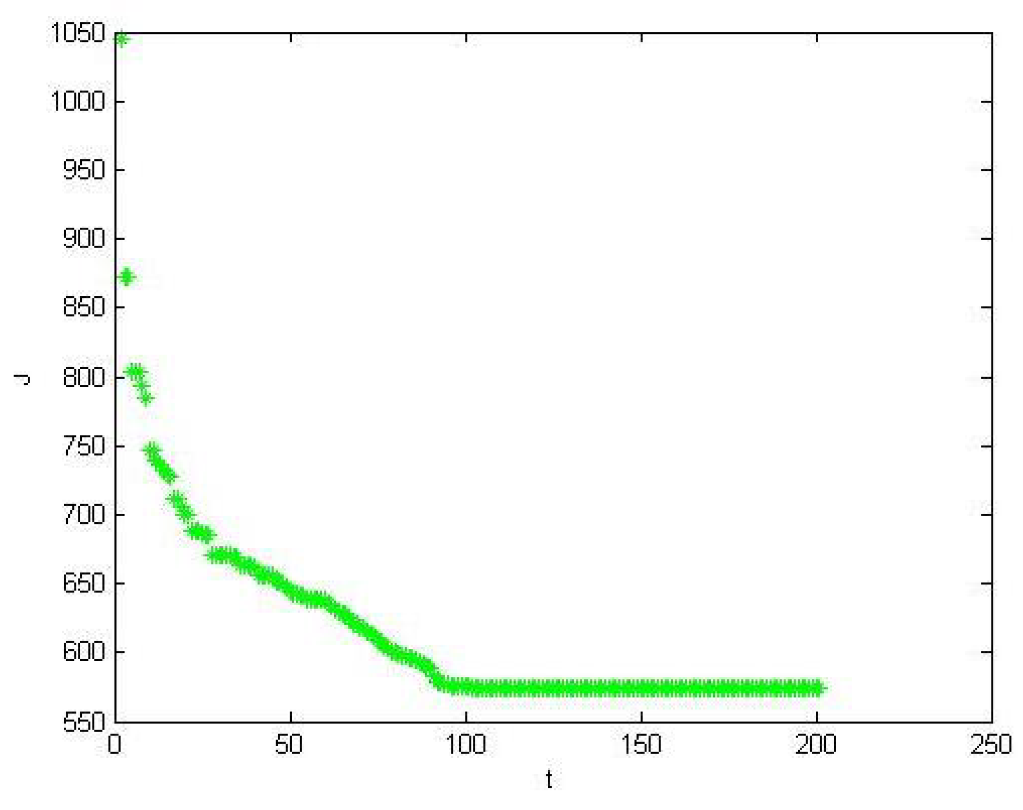
4. Optimization of Control Parameters

In the previous section, the FTCS conditions for networks (6) and (8) were established. Then, one can choose control parameters based on Equations (16) and (17) in Theorem 1. However, these equations only specify the range of the control parameters, which could lead to inefficient use of control resources if the parameters are chosen arbitrarily. To address this issue, an optimization model is developed and solved by PSO.

4.1. The Optimization Model

The optimization model of control parameters is structured as follows:

$$\begin{array}{cc}\hfill min& J={\displaystyle \frac{1}{2}}{\int }_{t_0}^{t^{\ast }}(e^H\left(t\right)e\left(t\right)+u^H\left(t\right)u\left(t\right))dt,\hfill \end{array}$$

(39)

$$\begin{array}{cc}\hfill s.t.{\lambda }_1>& 0,\hfill \end{array}$$

(40)

$$\begin{array}{cc}\hfill {\lambda }_2>& 0,\hfill \end{array}$$

(41)

$$\begin{array}{cc}\hfill k_i^1\ge & 0,i=1,2,\cdots ,N,\hfill \end{array}$$

(42)

$$\begin{array}{cc}\hfill k_j^2\ge & 0,j=1,2,\cdots ,n,\hfill \end{array}$$

(43)

$$\begin{array}{cc}\hfill t^{\ast }=& t_0+{\left(-{\displaystyle \frac{\varpi }{{\lambda }_1}}\right)}^{{\displaystyle \frac{1}{\alpha }}},\hfill \end{array}$$

(44)

$$\begin{array}{cc}\hfill \varpi =& max\left\{y|E_{\alpha }\left(y\right)={\displaystyle \frac{{\lambda }_2}{{\lambda }_1{\left|e\left(t_0\right)\right|}_1+{\lambda }_2}}\right\},\hfill \end{array}$$

(45)

where $u\left(t\right)={(u_1^T\left(t\right),u_2^T\left(t\right),\cdots ,u_N^T\left(t\right))}^T$, $e\left(t\right),{\lambda }_1,{\lambda }_2,k_i^1,k_j^2$ are same with Theorem 1. Equation (39) is the optimized target function [15], in which ${\displaystyle \frac{1}{2}}{\int }_{t_0}^{t^{\ast }}\left(e^H\left(t\right)e\left(t\right)\right)dt$ is the integral square error index, and ${\displaystyle \frac{1}{2}}{\int }_{t_0}^{t^{\ast }}\left(u^H\left(t\right)u\left(t\right)\right)dt$ represents the control energy. The target is to minimize the sum of these two terms. Equations (40)–(45) serve as the constraint conditions, with Equations (40) and (41) corresponding to the FTCS conditions outlined in Theorem 1. An algorithm based on the PSO method is designed to solve this complicated optimization model.

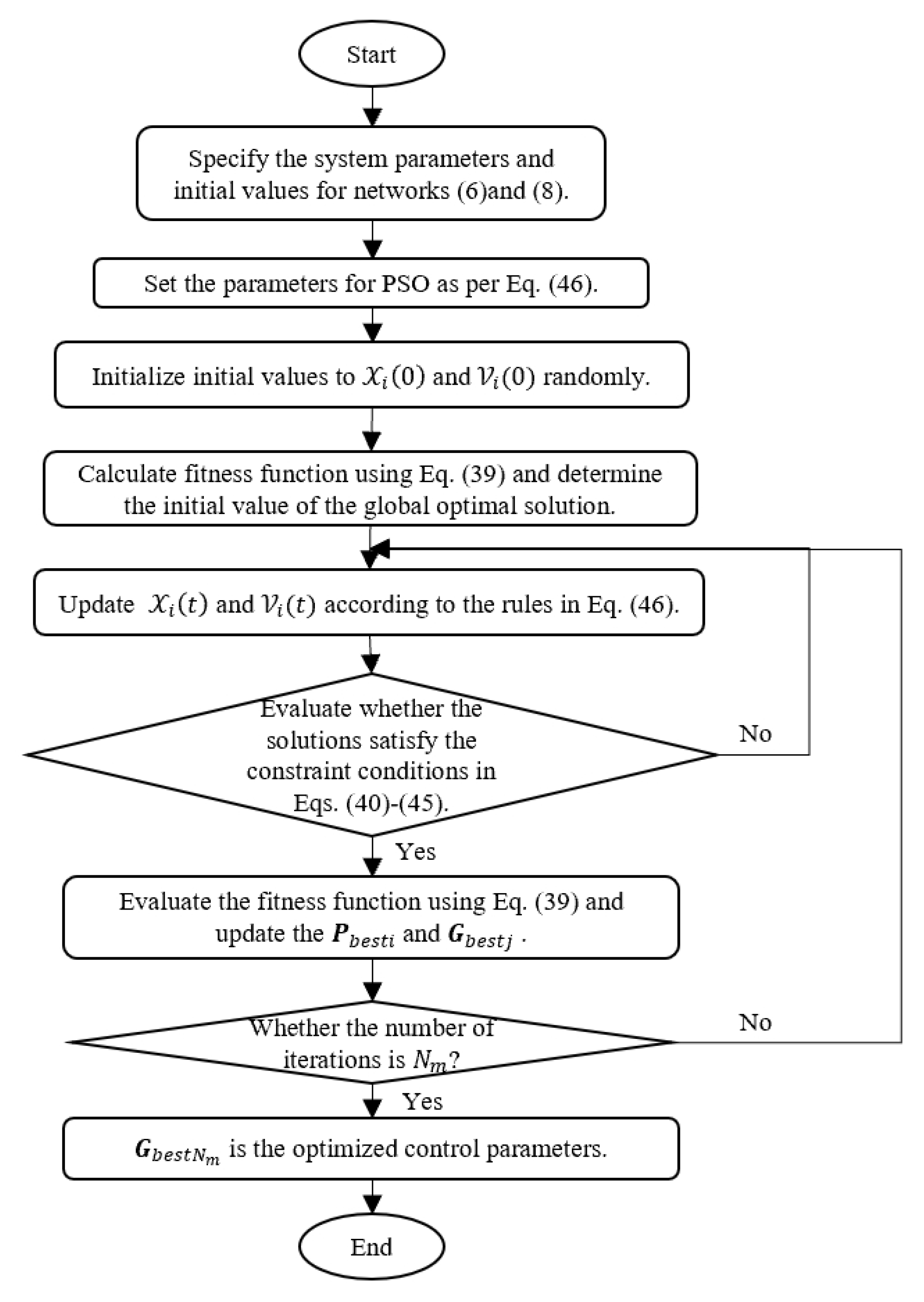
4.2. An Algorithm with PSO

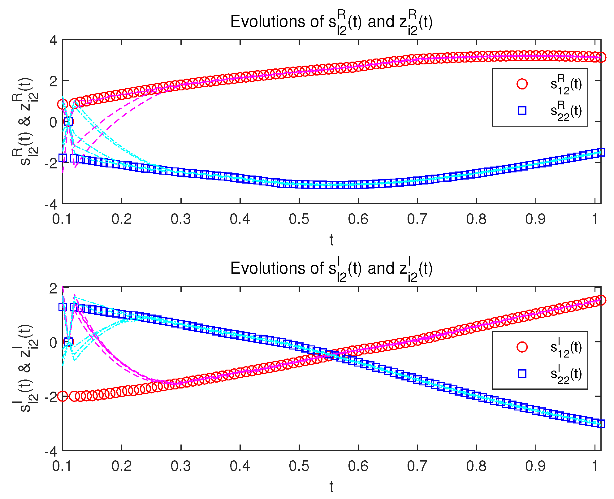
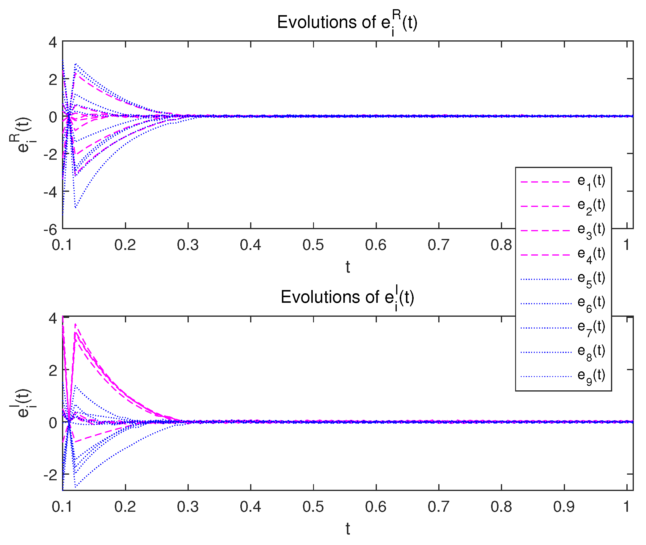
The PSO algorithm is a classical intelligent optimization technique that leverages the collective intelligence of a group to find the optimal solution. In this algorithm, a large number of particles are iteratively updated. Each particle has its own velocity and position, where the position represents the value of a potential solution, and the velocity updates the position in each iteration. The velocity update is guided by the particle’s historical best position ${\mathbf{P}}_{best}$ and the global best position ${\mathbf{G}}_{best}$. The following outlines the rules for updating position and velocity:

$$\begin{array}{cc}\hfill {\mathcal{X}}_i(t+1)=& {\mathcal{X}}_i\left(t\right)+{\mathcal{V}}_i(t+1),\hfill \\ \hfill {\mathcal{V}}_i(t+1)=& w\left(t\right){\mathcal{V}}_i\left(t\right)+c_{1}ran{d}_1({\mathbf{P}}_{besti}\left(t\right)-{\mathcal{X}}_i\left(t\right))+c_{2}ran{d}_2({\mathbf{G}}_{bestj}\left(t\right)-{\mathcal{X}}_i\left(t\right)),\hfill \end{array}$$

(46)

where ${\mathcal{V}}_i\left(t\right)={({\mathcal{V}}_{i1}\left(t\right),{\mathcal{V}}_{i2}\left(t\right),\cdots ,{\mathcal{V}}_{i(N+n)}\left(t\right))}^T\in {\mathbb{R}}^{N+n}$ is the velocity vector of the ith particle, ${\mathcal{X}}_i\left(t\right)={({\mathcal{X}}_{i1}\left(t\right),{\mathcal{X}}_{i2}\left(t\right),\cdots ,{\mathcal{X}}_{i(N+n)}\left(t\right))}^T\in {\mathbb{R}}^{N+n}$ is the position vector of the ith particle at the tth iteration. $N+n$ represents the size of the solution space. $i=1,2,\cdots ,\mathcal{M}$, $\mathcal{M}$ denotes particle size. $w\left(t\right)$ represents the inertia weight, which is randomly chosen from $(0.4,0.9)$. $c_1,c_2$, $ran{d}_1$ and $ran{d}_2$ are constants. ${\mathbf{P}}_{besti}\left(t\right)={(p_{besti1},p_{besti2},\cdots ,p_{besti(N+n)})}^T$ is the historical optimal position vector of ith particle. ${\mathbf{G}}_{bestj}\left(t\right)={(g_{bestj1},g_{bestj2},\cdots ,g_{bestj(N+n)})}^T$ is the global optimal position vector of the jth iteration, $j=1,2,\cdots ,N_m$, $N_m$ is the maximum iterations.

To address the optimization model presented in Section 4.1, a novel algorithm is developed based on PSO. The flow chart of the algorithm is outlined in Figure 1.

Figure 1. The flow chart of control parameters selection algorithm based on PSO.

Remark 4.

There is a negative feedback control with CVSF in [31,32]. However, these papers only provide a range for the control parameters, such as $k_i^1,k_i^2\ge X$, where X is a non-negative constant, leaving the selection of specific control parameters within this range up to the user. The method outlined in this paper facilitates the calculation of control parameters aimed at minimizing the combined costs of control energy and dynamic errors, providing a more economical strategy for selecting control parameters in FCCMNN. This algorithm is based on PSO algorithm and combined the Theorem 1’s conditions. It is not a global optimal algorithm and still has some limitations, but it can give a method to select the optimized control parameters.

5. Simulation

5.1. Example 1

There is an example to demonstrate the feasibility of the main result and the optimization method. The leader’s dynamical network (8) is that:

$$\begin{array}{cc}\hfill D_{t_0,t}^{\alpha }{s}_l\left(t\right)=& -C{s}_l\left(t\right)+A\left(s_l\left(t\right)\right)f\left(s_l\left(t\right)\right)+B\left(s_l\left(t\right)\right)f\left(s_l(t-\tau )\right)+I\left(t\right).\hfill \end{array}$$

(47)

Let fractional-order $\alpha =0.97$, the dimension of neuronal states $n=2$, the number of clusters $m=2$. The initial values are $s_1={(-1.05-\mathbf{i},0.8-2\mathbf{i})}^T,s_2={(2.74+1.05\mathbf{i},-1.75+1.31\mathbf{i})}^T$. $C=diag(0.4-3.07\mathbf{i},0.2-1.43\mathbf{i})$, $f\left(s\left(t\right)\right)=tanh\left(s^R\left(t\right)\right)+tanh\left(s^I\left(t\right)\right)\mathbf{i}$, then $L=1$ and $F=2$. Let $\tau =0.1$, $I\left(t\right)=0.1sin\left(t\right)+0.3cos\left(t\right)\mathbf{i}$.

$$a_{11}\left(y_1\right)=\left\{\begin{array}{ccc}\hfill -1.24-1.75\mathbf{i},& & \hfill |y_1{|}_1\le 3,\\ \hfill -1.3-1.13\mathbf{i},& & \hfill |y_1{|}_1>3,\end{array}\right.a_{12}\left(y_1\right)=\left\{\begin{array}{ccc}\hfill -2.17-1.89\mathbf{i},& & \hfill |y_1{|}_1\le 3,\\ \hfill -2.22-1.99\mathbf{i},& & \hfill |y_1{|}_1>3,\end{array}\right.$$

$$a_{21}\left(y_2\right)=\left\{\begin{array}{ccc}\hfill -1.56+1.69\mathbf{i},& & \hfill |y_2{|}_1\le 3,\\ \hfill -1.62+1.87\mathbf{i},& & \hfill |y_2{|}_1>3,\end{array}\right.a_{22}\left(y_2\right)=\left\{\begin{array}{ccc}\hfill 1.43-0.44\mathbf{i},& & \hfill |y_2{|}_1\le 3,\\ \hfill 1.3-0.06\mathbf{i},& & \hfill |y_2{|}_1>3,\end{array}\right.$$

$$b_{11}\left(y_1\right)=\left\{\begin{array}{ccc}\hfill 0.06+0.31\mathbf{i},& & \hfill |y_1{|}_1\le 3,\\ \hfill -0.03+0.25\mathbf{i},& & \hfill |y_1{|}_1>3,\end{array}\right.b_{12}\left(y_1\right)=\left\{\begin{array}{ccc}\hfill -0.31+0.09\mathbf{i},& & \hfill |y_1{|}_1\le 3,\\ \hfill 0.22-0.07\mathbf{i},& & \hfill |y_1{|}_1>3,\end{array}\right.$$

$$b_{21}\left(y_2\right)=\left\{\begin{array}{ccc}\hfill 0.03+0.44\mathbf{i},& & \hfill |y_2{|}_1\le 3,\\ \hfill 0.09+0.07\mathbf{i},& & \hfill |y_2{|}_1>3,\end{array}\right.b_{22}\left(y_2\right)=\left\{\begin{array}{ccc}\hfill -0.1+0.08\mathbf{i},& & \hfill |y_2{|}_1\le 3,\\ \hfill -2.21-0.07\mathbf{i},& & \hfill |y_2{|}_1>3.\end{array}\right.$$

The two-dimensional (2D) state curves of $s\left(t\right)$ are shown in Figure 2. The network (6) with the controller (14) is that:

$$\begin{array}{cc}\hfill D_{t_0,t}^{\alpha }{z}_i\left(t\right)=& -C{z}_i\left(t\right)+A\left(z_i\left(t\right)\right)f\left(z_i\left(t\right)\right)+B\left(z_i\left(t\right)\right)f\left(z_i(t-\tau )\right)+\sigma \sum _{j=1}^N{g}_{ij}\Gamma z_j\left(t\right)+I\left(t\right)\hfill \\ & -k_i^1{e}_i\left(t\right)-k_i^2\left[e_i\left(t\right)\right],\hfill \end{array}$$

(48)

where the strength of coupling $\sigma =1.5$, $\Gamma =diag(0.2,0.2)$. The topology of the network (6) is in Figure 3. The solid line represents a connection weight of 1, while the dashed line denotes $-1$. The nine neurons are divided into two clusters. ${\Lambda }_1=\{1,2,3,4\}$, ${\Lambda }_2=\{5,6,7,8,9\}$. By calculation, one can have $\widehat{C}=diag(-2.67,-1.23)$. Select $K^1=diag(9.87,10.17,10.47,9.87,9.87,9.87,10.47,9.87,10.17)$ and $K^2=diag(4.84,4.6)$. Then, ${\lambda }_1=1.4807>0$, ${\lambda }_2=0.1>0$. Let $t_0=0$, the initial value of $z_{ip}(i=1,2,\cdots ,9,p=1,2)$ is selected randomly from $[-2,2]+[-2,2]\mathbf{i}$. Based on Theorem 1, one can calculate that $|e\left(t_0\right){|}_1=67.5107$, $\varpi =-32.47$, $t^{\ast }=24.1267$.

$$\overline{A}=\left(\begin{array}{cc}2.99& 4.21\\ 3.49& 1.87\end{array}\right),\overline{B}=\left(\begin{array}{cc}0.37& 0.4\\ 0.47& 0.28\end{array}\right),\tilde{A}=\left(\begin{array}{cc}0.68& 0.15\\ 0.24& 0.51\end{array}\right).$$

Figure 2. The 2D state curves of the leaders $s_1\left(t\right)$ and $s_2\left(t\right)$ of 2 clusters in Example 1.

Figure 3. The topology of 9 neurons of the network (6) in Example 1.

The states of $s_l\left(t\right)(l=1,2)$ and $z_i\left(t\right)(i=1,2,\cdots ,9)$ are shown in Figure 4 and Figure 5 under the controller (14). The red circle represents $s_1\left(t\right)$, the blue square is $s_2\left(t\right)$. The magenta double lines indicate neurons 1-4 belonging to the first cluster and all the dot dash lines in cyan indicate neurons 5-9 belonging to the second cluster. Obviously, they can achieve the FTCS, and the settling time is less than $t^{\ast }$ in practice. The error systems are shown in Figure 6. In this figure, all magenta double lines represent the neurons belonging to the first cluster, and blue dotted lines represent the neurons belonging to the second cluster. As time goes by, the systematic errors tend to 0.

Figure 4. The stable evolution of the first dimensional state of the leaders $s_{l1}\left(t\right)$ and follower-neurons $z_{i1}\left(t\right)$ in Example 1, $l=1,2$, $i=1,2,\cdots ,9$.

Figure 5. The stable evolution of the second dimensional state of the leaders $s_{l2}\left(t\right)$ and follower-neurons $z_{i2}\left(t\right)$ in Example 1, $l=1,2$, $i=1,2,\cdots ,9$.

Figure 6. The stable evolutions of 9 neurons’ errors $e_i\left(t\right)$ in Example 1, $i=1,2,\cdots ,9$.

The following is the optimization part of the control parameters. There are some parameters for the PSO algorithm. Let $M=50$, $N_m=200$, $c_1=c_2=2$. Figure 7 describes the value of the fitness function (target function) J corresponding to the global optimal solution ${\mathbf{G}}_{best}$ during each iteration. Along with the increasing iteration times, the value of J becomes lower and lower. One can obtain the optimized control parameters, and the relevant J is $573.7228$ in this simulation.

Figure 7. The evolution of optimization target function J in Example 1.

There is a comparison experiment. The control parameters with and without the provided optimization algorithm are stated in Table 2. Most papers only give the range of control parameters, that is to say, the control parameters need to satisfy the conditions of Theorem 1. This method is expressed by the Normal method. The control gains is selected as $k_1^1=9.87$, $k_2^1=10.17$, $k_3^1=10.47$, $k_4^1=9.87$, $k_5^1=9.87$, $k_6^1=9.87$, $k_7^1=10.47$, $k_8^1=9.87$, $k_9^1=10.17$, $k_1^2=4.84$, $k_2^2=4.6$, in this method, which satisfy the Theorem 1, and the sum of ISE and control energy is 691.2507. This paper proposes an optimization method of control parameters, which is called the optimization method. The control parameters obtained according to the algorithm proposed in this paper is $k_1^1=10.6886$, $k_2^1=1.3105\times {10}^{-4}$, $k_3^1=8.6932$, $k_4^1=8.2978$, $k_5^1=9.6064$, $k_6^1=8.4519$, $k_7^1=0.0408$, $k_8^1=10.643$, $k_9^1=10.355$, $k_1^2=5.6879$, $k_2^2=3.7145$ and the optimization objective is 573.7228. The control parameters and the provided optimization algorithm can obtain a lower sum of control energy and ISE index. Therefore, this optimization method can guide the selection of the control parameters.

Table 2. Results with different control parameters in Example 1.

Method		Control	Parameters		J
Normal	$k_i^1,i=1\to 3$	9.87	10.17	10.47	691.2507
	$k_i^1,i=4\to 6$	9.87	9.87	9.87
	$k_i^1,i=7\to 9$	10.47	9.87	10.17
	$k_i^2,i=1,2$	4.84	4.6
Optimization	$k_i^1,i=1\to 3$	10.6886	$1.3105\times {10}^{-4}$	8.6932	573.7228
	$k_i^1,i=4\to 6$	8.2978	9.6064	8.4519
	$k_i^1,i=7\to 9$	0.0408	10.643	10.355
	$k_i^2,i=1,2$	5.6879	3.7145

Remark 5.

The control matrix $K^1$ can let the matrix ${\Xi }_1=I_N\otimes (\widehat{C}-L\overline{A})-\sigma \overline{G}\otimes \Gamma +K^1\otimes I_n$ in Equation (16) is a diagonally-dominant matrix. At the same time, $K^1$ has the minimum norm in the normal method of the comparison experiment. The selection of control matrices in [32] is similar to the normal method in this paper. Since the optimization of the controller is not considered in [32], the controller is not the minimum norm matrix that can make the matrix of synchronization condition is a diagonally dominant matrix in the simulation. However, the proposed optimization method can give better control parameters than the parameters via the normal method. That is to say, the proposed optimization method is better than an arbitrary selection within a certain range.

Remark 6.

In this example, the “tanh” function is used as an activation function. In fact, all functions which satisfy Assumption 2 can be used as the activation function.

5.2. Example 2

There is a comparison experiment with [31] to further illustrate the advantage of the optimization method. The studied model is the same with Example 1 in [31]. The leader’s state of each cluster is

$$D_{0,t}^{\alpha }{s}_l\left(t\right)=-C{s}_l\left(t\right)+Bf\left(s_l\left(t\right)\right),$$

(49)

where $l=1,2$.

The CNN without memristor is described as follows:

$$\begin{array}{cc}\hfill D_{0,t}^{\alpha }{z}_i\left(t\right)=& -C{z}_i\left(t\right)+Bf\left(z_i\left(t\right)\right)+\sum _{j=1}^N{g}_{ij}h\left(z_j\left(t\right)\right)-d_l{e}_i\left(t\right)-{\theta }_l\left[e_i\left(t\right)\right],\hfill \end{array}$$

(50)

where $N=14$, ${\Lambda }_1=\{1,2,\cdots ,7\}$, ${\Lambda }_2=\{8,9,\cdots ,14\}$. When $i\in {\Lambda }_1, l=1$, otherwise, $l=2$. $f\left(s\left(t\right)\right)=tanh\left(s^R\left(t\right)\right)+tanh\left(s^I\left(t\right)\right)\mathbf{i}$, $h\left(s\left(t\right)\right)=0.1\times {\displaystyle \frac{1-exp(-s{\left(t\right)}^R)}{1+exp(-s{\left(t\right)}^R)}}+{\displaystyle \frac{0.1}{1+exp(-s{\left(t\right)}^I)}}\mathbf{i}$.

The topology of the network (50) is in Figure 8. If neurons i and j can connect with each other, $g_{ij}=1$, otherwise, $g_{ij}=0$, besides, $g_{ii}=-{\sum }_{j=1}^n{g}_{ij}$. The parameters are identical to Case 2 of Example 1 in [31], such as $\alpha =0.7,$ $d_1=9,$ $d_2=8,$ ${\theta }_1={\theta }_2=5$. The matrices C and B, and the initial value of $s_l\left(t\right)$ are omitted here, which can be found in [31]. In [31], the settling time is 7.6398, and by calculation, the value of J in Equation (39) is $3.7505\times {10}^3$. We replaced the synchronization conditions of the optimization model in Section 4.1 with the synchronization conditions of Theorem 2 in [31]. The parameters of the optimization algorithm are $M=50$, $N_m=100$, $c_1=c_2=1$, and we solved the optimization model with the step in Section 4.2. Then we found the optimal control parameters are $d_1=13.8477,$ $d_2=13.8515,$ ${\theta }_1=2.5530,$ ${\theta }_2=2.5525$. Accordingly, the settling time is 7.5698, and the value of the fitness function J is $2.8144\times {10}^3$. The results of the comparison experiment are shown in Table 3 detailedly. Obviously, the settling times are close, but the values of J are $2.8144\times {10}^3<3.7505\times {10}^3$, which substantiate the proposed optimization method can help to select better control parameters, which can save control resources greatly.

Table 3. Results of comparison experiment in Example 2.

Method	${\mathit{d}}_1$	${\mathit{d}}_2$	${\mathit{\theta }}_1$	${\mathit{\theta }}_2$	${\mathit{t}}^{\ast }$	J
[31]	9	8	5	5	7.6398	$3.7505\times {10}^3$
Optimization	13.8477	13.8515	2.5530	2.5525	7.5698	$2.8144\times {10}^3$

Figure 8. The topology of 14 neurons of the network (50) in Example 2.

Figure 8. The topology of 14 neurons of the network (50) in Example 2.

Remark 7.

A lot of papers [13,14,18,20,21,23,31,32,33,37] only pay attention to the synchronization of the networks, they can give the range of control parameters, but our optimization method can select the optimal control parameters and obtain an energy-efficient controller.

6. Conclusions

This paper investigates a coupled neural network based on a memristor, specifically a FOCV system with a time delay. The FTCS of these networks is analyzed, with neurons divided into different clusters, each following distinct leaders. A controller using the CVSF is designed to achieve FTCS without decomposition. Additionally, an optimization model solved by PSO is developed, guiding the selection of control parameters. The simulation results verify the proposed theorem and optimization method. This work successfully achieves FTCS for fractional-order complex systems. The advantage of the proposed theorem is that the FTCS of FOCV neural networks can be achieved without dividing the complex values into real and imaginary parts. Additionally, the model studied in this paper is more extensive, and the special case of the theorem is the conclusion in other literature, which is challenging. The advantage of the proposed algorithm is that the method of selecting control parameters can be given on the basis of the theorem, which makes up for the lack of research. However, the settling time of FTCS is influenced by the systems’ initial values, which is difficult to obtain sometimes. Therefore, achieving fixed-time synchronization, where the settling time is independent of initial values, remains an area for future research, particularly for FOCV systems, which are not yet well-explored. That will be our future study.

References

1. lghamdi, F.A.; Almanaseer, H.; Jaradat, G.; Jaradat, A.; Alsmadi, M.K.; Jawarneh, S.; Almurayh, A.S.; Alqurni, J.; Alfagham, H. Multilayer perceptron neural network with arithmetic optimization algorithm-based feature selection for cardiovascular disease prediction. Mach. Learn. Knowl. Extr. 2024, 6, 987–1008. [Google Scholar] [CrossRef]
2. Luo, N.; Xu, D.; Xing, B.; Yang, X.; Sun, C. Principles and applications of convolutional neural network for spectral analysis in food quality evaluation: A review. J. Food Compos. Anal. 2024, 128, 105996. [Google Scholar] [CrossRef]
3. Zhao, B.; Cao, X.; Zhang, W.; Liu, X.; Miao, Q.; Li, Y. CompNET: Boosting image recognition and writer identification via complementary neural network post-processing. Pattern Recognit. 2025, 157, 110880. [Google Scholar] [CrossRef]
4. Park, J.H. Recent Advances in Control Problems of Dynamical Systems and Networks; Springer-Nature: Cham, Switzerland, 2021. [Google Scholar]
5. Lai, Q.; Yang, L.; Hu, G.; Guan, Z.-H.; Iu, H.H.-C. Constructing multiscroll memristive neural network with local activity memristor and application in image encryption. IEEE Trans. Cybern. 2024, 54, 4039–4048. [Google Scholar] [CrossRef]
6. Liu, H.; Cheng, J.; Cao, J.; Katib, I. Preassigned-time synchronization for complex-valued memristive neural networks with reaction–diffusion terms and Markov parameters. Neural Netw. 2024, 169, 520–531. [Google Scholar] [CrossRef]
7. Zhang, Y.; Zhou, L. State estimation for proportional delayed complex-valued memristive neural networks. Inf. Sci. 2024, 680, 121150. [Google Scholar] [CrossRef]
8. Chang, Q.; Park, J.H.; Yang, Y. The optimization of control parameters: Finite-time bipartite synchronization of memristive neural networks with multiple time delays via saturation function. IEEE Trans. Neural Networks Learn. Syst. 2022, 34, 7861–7872. [Google Scholar] [CrossRef]
9. Aguirre, F.; Sebastian, A.; Le Gallo, M.; Song, W.; Wang, T.; Yang, J.J.; Lu, W.; Chang, M.-F.; Ielmini, D.; Yang, Y.; et al. Hardware implementation of memristor-based artificial neural networks. Nat. Commun. 2024, 15, 1974. [Google Scholar] [CrossRef]
10. Zhang, G.; Wen, S. New approximate results of fixed-time stabilization for delayed inertial memristive neural networks. IEEE Trans. Circuits Syst. II Express Briefs 2024, 71, 3428–3432. [Google Scholar] [CrossRef]
11. Deng, Q.; Wang, C.; Lin, H. Memristive Hopfield neural network dynamics with heterogeneous activation functions and its application. Chaos Solitons Fractals 2024, 178, 114387. [Google Scholar] [CrossRef]
12. Li, Y.; Chen, Y.; Podlubny, I. Mittag–Leffler stability of fractional order nonlinear dynamic systems. Automatica 2009, 45, 1965–1969. [Google Scholar] [CrossRef]
13. Panda, S.K.; Nagy, A.; Vijayakumar, V.; Hazarika, B. Stability analysis for complex-valued neural networks with fractional order. Chaos Solitons Fractals 2023, 175, 114045. [Google Scholar] [CrossRef]
14. Feng, L.; Yu, J.; Hu, C.; Yang, C.; Jiang, H. Nonseparation method-based finite/fixed-time synchronization of fully complex-valued discontinuous neural networks. IEEE Trans. Cybern. 2020, 51, 212–3223. [Google Scholar] [CrossRef]
15. Chang, Q.; Park, J.H.; Yang, Y.; Wang, F. Finite-Time multiparty synchronization of T–S fuzzy coupled memristive neural networks with optimal event-triggered control. IEEE Trans. Fuzzy Syst. 2022, 31, 2545–2555. [Google Scholar] [CrossRef]
16. Sorrentino, F.; Pecora, L.M.; Hagerstrom, A.M.; Murphy, T.E.; Roy, R. Complete characterization of the stability of cluster synchronization in complex dynamical networks. Sci. Adv. 2016, 2, e1501737. [Google Scholar] [CrossRef] [PubMed]
17. Rossa, F.D.; Pecora, L.; Blaha, K.; Shirin, A.; Klickstein, I.; Sorrentino, F. Symmetries and cluster synchronization in multilayer networks. Nat. Commun. 2020, 11, 3179. [Google Scholar] [CrossRef]
18. Zhou, L.; Tan, F.; Yu, F.; Liu, W. Cluster synchronization of two-layer nonlinearly coupled multiplex networks with multi-links and time-delays. Neurocomputing 2019, 359, 264–275. [Google Scholar] [CrossRef]
19. Tang, Z.; Park, J.H.; Shen, H. Finite-time cluster synchronization of lur’e networks: A nonsmooth approach. IEEE Trans. Syst. Man Cybern. Syst. 2018, 48, 1213–1224. [Google Scholar] [CrossRef]
20. Zhang, Z.; Liu, X.; Zhou, D.; Lin, C.; Chen, J.; Wang, H. Finite-time stabilizability and instabilizability for complex-valued memristive neural networks with time delays. IEEE Trans. Syst. Man Cybern. Syst. 2018, 48, 2371–2382. [Google Scholar] [CrossRef]
21. Chen, J.; Chen, B.; Zeng, Z. Global asymptotic stability and adaptive ultimate mittag-leffler synchronization for a fractional-order complex-valued memristive neural networks with delays. IEEE Trans. Syst. Man Cybern. Syst. 2019, 49, 2519–2535. [Google Scholar] [CrossRef]
22. Li, X.; Wu, H.; Cao, J. Synchronization in finite time for variable-order fractional complex dynamic networks with multi-weights and discontinuous nodes based on sliding mode control strategy. Neural Netw. 2021, 139, 335–347. [Google Scholar] [CrossRef] [PubMed]
23. Duan, L.; Shi, M.; Huang, C.; Fang, X. Synchronization in finite-/fixed-time of delayed diffusive complex-valued neural networks with discontinuous activations. Chaos Solitons Fractals 2021, 142, 110386. [Google Scholar] [CrossRef]
24. Kennedy, J.; Eberhart, R. Particle swarm optimization. In Proceedings of the ICNN’95-International Conference on Neural Networks, Perth, WA, Australia, 27 November–1 December 1995; Volume 4, pp. 1942–1948. [Google Scholar]
25. Tan, Y.; Yuan, Y.; Xie, X.; Tian, E.; Liu, J. Observer-based event-triggered control for interval type-2 fuzzy networked system with network attacks. IEEE Trans. Fuzzy Syst. 2023, 31, 2788–2798. [Google Scholar] [CrossRef]
26. Liu, B.; Liu, T.; Xiao, P. Dynamic event-triggered intermittent control for stabilization of delayed dynamical systems. Automatica 2023, 149, 110847. [Google Scholar] [CrossRef]
27. Li, X.; Liu, W.; Gorbachev, S.; Cao, J. Event-triggered impulsive control for input-to-state stabilization of nonlinear time-delay systems. IEEE Trans. Cybern. 2023, 54, 2536–2544. [Google Scholar] [CrossRef]
28. Liu, Z.; Gao, H.; Yu, X.; Lin, W.; Qiu, J.; Rodríguez-Andina, J.J.; Qu, D. B-spline wavelet neural-network-based adaptive control for linear-motor-driven systems via a novel gradient descent algorithm. IEEE Trans. Ind. Electron. 2023, 71, 1896–1905. [Google Scholar] [CrossRef]
29. Wang, J.; Ru, T.; Shen, H.; Cao, J.; Park, J.H. Finite-time L2L synchronization for semi-markov jump inertial neural networks using sampled data. IEEE Trans. Network Sci. Eng. 2021, 8, 163–173. [Google Scholar] [CrossRef]
30. Park, J.H.; Lee, T.H.; Liu, Y.; Chen, J. Dynamic Systems with Time Delays: Stability and Control; Springer-Nature: Singapore, 2019. [Google Scholar]
31. Yang, S.; Hu, C.; Yu, J.; Jiang, H. Finite-time cluster synchronization in complex-variable networks with fractional-order and nonlinear coupling. Neural Netw. 2021, 135, 212–224. [Google Scholar] [CrossRef] [PubMed]
32. Liu, P.; Zeng, Z.; Wang, J. Asymptotic and finite-time cluster synchronization of coupled fractional-order neural networks with time delay. IEEE Trans. Neural Netw. Learn. Syst. 2020, 31, 4956–4967. [Google Scholar] [CrossRef]
33. Wang, L.; Song, Q.; Liu, Y.; Zhao, Z.; Alsaadi, F.E. Finite-time stability analysis of fractional-order complex-valued memristor-based neural networks with both leakage and time-varying delays. Neurocomputing 2017, 245, 86–101. [Google Scholar] [CrossRef]
34. Yu, T.; Cao, J.; Rutkowski, L.; Luo, Y.-P. Finite-time synchronization of complex-valued memristive-based neural networks via hybrid control. IEEE Trans. Neural Netw. Learn. Syst. 2021, 33, 3938–3947. [Google Scholar] [CrossRef] [PubMed]
35. Zhu, X.; Tang, Z.; Feng, J.; Park, J.H. Aperiodically intermittent event-triggered pinning control on cluster synchronization of directed complex networks. ISA Trans. 2023, 138, 281–290. [Google Scholar] [CrossRef]
36. Zhang, J.; Ma, Z.; Li, X.; Qiu, J. Cluster Synchronization in Delayed Networks With Adaptive Coupling Strength via Pinning Control. Front. Phys. 2020, 8, 235. [Google Scholar] [CrossRef]
37. Hou, T.; Yu, J.; Hu, C.; Jiang, H. Finite-time synchronization of fractional-order complex-variable dynamic networks. IEEE Trans. Syst. Man Cybern. Syst. 2019, 51, 4297–4307. [Google Scholar] [CrossRef]
38. Podlubny, I. Fractional Differential Equations; Academic Press: London, UK, 1999. [Google Scholar]