Hyperbolic Sine Function Control-Based Finite-Time Bipartite Synchronization of Fractional-Order Spatiotemporal Networks and Its Application in Image Encryption

Abstract

This work is devoted to the hyperbolic sine function (HSF) control-based finite-time bipartite synchronization of fractional-order spatiotemporal networks and its application in image encryption. Initially, the addressed networks adequately take into account the nature of anisotropic diffusion, i.e., the diffusion matrix can be not only non-diagonal but also non-square, without the conservative requirements in plenty of the existing literature. Next, an equation transformation and an inequality estimate for the anisotropic diffusion term are established, which are fundamental for analyzing the diffusion phenomenon in network dynamics. Subsequently, three control laws are devised to offer a detailed discussion for HSF control law’s outstanding performances, including the swifter convergence rate, the tighter bound of the settling time and the suppression of chattering. Following this, by a designed chaotic system with multi-scroll chaotic attractors tested with bifurcation diagrams, Poincaré map, and Turing pattern, several simulations are pvorided to attest the correctness of our developed findings. Finally, a formulated image encryption algorithm, which is evaluated through imperative security tests, reveals the effectiveness and superiority of the obtained results.

1. Introduction

Recent years have witnessed the flourishing development of complex networks (CNs) across diverse fields, encompassing social networks [1], power grids [2] and transportation networks [3]. Synchronization, a fundamental issue in the dynamic analysis of CNs, in which all nodes should achieve a desired performance, has attracted extensive attention from scholars. The theories and techniques developed in synchronization analyses have already been successfully applied in a broad scope of fields, such as secure communication [4], biological engineering [5] and image encryption [6]. Notably, there is a widespread occurrence of diffusion phenomena with spatiotemporal properties in practical engineering scenarios, including electrons moving in a circuit to implement a neural network and the substance concentration changes that occur during chemical reactions. Therefore, CNs with a reaction term and a diffusion term, i.e., spatiotemporal networks (SNs), have captured much attention of the scholars, and some fascinating and remarkable achievements have been published [7,8,9]. Nevertheless, the aforementioned works on SNs are all based on the premise that the diffusion matrix should be diagonal, posing extremely strict restrictions regarding the scope of their practical applications. Besides, there are few related works on the synchronization of SNs with anisotropic diffusion, i.e., the diffusion matrix in a general form. Hence, it is challenging but urgent to address this problem, as this would provide significant guidance in dynamic behavior analyses of SNs, which is the starting point of this work.

In another respect, due to the positive qualities of heritability and finite memory, fractional calculus has attracted widespread research interest and has already been extensively employed in various fields, including image enhancement [10], viscoelastic systems [11], and Lithium–ion batteries [12]. Therefore, it is of great significance to discuss fractional calculus in both theory and practice. Since fractional calculus was incorporated into networks, abundant remarkable accomplishments have been obtained in fractional-order (FO) networks [13,14,15]. Notably, Wu et al. [13] established an FO partial differential inequality to solve the pinning synchronization of multiple FO fuzzy complex-valued delayed spatiotemporal neural networks using a decomposition approach. In [14], projective synchronization was analyzed for FO neural networks with mixed time delays using the extended Halanay inequality. However, findings regarding the synchronization of FOSN appear limited, which prompted us to further explore this interesting and meaningful problem.

Significantly, the focus of the above-mentioned works is networks with only positive weights, meaning that the nodes in the networks are just only cooperative. In fact, competition exists in almost all complex systems, such as different companies competing for economic benefits and different countries competing to obtain military dominance. As a consequence, it is highly valuable to consider the synchronization of networks featuring both cooperation and competition. Additionally, ever since the publication of Altafini’s pioneering work [16], bipartite synchronization (BS), in which a subset of the nodes synchronize to a desired state while the remaining nodes synchronize to the same value with the opposite sign, this has quickly emerged as a major research issue [17,18,19,20]. Xu et al. [17] devised a hybrid impulsive to study the exponential BS of FO multilayer signed networks with both positive and negative impulsive effects. Ding et al. [18] discussed the quasi-BS of complex networks via memory-based self-triggered control. In [20], interval BS were studied in multiple neural networks with signed graphs. Nonetheless, academic studies involving the BS of FOSNs are relatively few, which strongly stimulated our research interest.

Another issue deserving attention is that the results set forth previously all concentrate on asymptotic synchronization over an infinite time scale. However, real tasks often must be finished within a limited window of time. Accordingly, based on a seminal work [21] regarding finite-time (FN) stability, FN synchronization, where all nodes converge to the desired performance within a limited window, quickly captured the attention of multiple researchers. FN synchronization has achieved a multitude of excellent outcomes [22,23,24,25], due to its distinct superiority in terms of its quick convergence rate, high control accuracy, and anti-interference qualities. In control research domains, how to more accurately estimate settling time (ST) has consistently been one of the most prominent research hotspots. Furthermore, the hyperbolic sine function (HSF), as a generalized exponential function with some trigonometric properties, plays a fascinating role in dynamic analysis. The systems in [26,27] based on the HSF exhibited intricate bifurcation and strange chaotic attractors. In [28], the HSF was introduced in sliding mode to solve the uncertain FO chaos synchronization. Following this, it is natural to consider why the HSF, with such admirable properties, could generate an excellent control effect in synchronization control. Fortunately, Xu et al. [29] devised a novel control scheme involving an HSF and a linear term to synchronize CN within a finite time, achieving a tighter bound of ST and anti-chattering abilities. However, the HSF control law has not gained the attention it deserves, and nor has the FNBS of FOSNs. The primary challenges are summarized as follows: (1) the spatial variability, anisotropic diffusion matrix, and diffusion term pose difficulties when designing a control scheme based on Taylor expansion and HSF; (2) as the HSF control is a relatively novel method, it is challenging to improve the control scheme in [29], and there is no straightforward method to decouple the reason for its outstanding anti-chattering qualities or its ability to achieve a tighter bound of ST. It is important to address these challenges, which was the primary motivation for this paper.

Sparked by the above discussions, the intention of the paper is to pursue the FNBS of FOSNs. The main achievements are summarized as follows:

(1) In contrast to the existing literature [7,30,31], which have relatively conservative requirements for diagonal diffusion matrices, the addressed FOSN, with anisotropic diffusion, is more in accordance with the actual circumstances, in which the diffusion matrix can be non-diagonal or non-square, i.e., the number of state components is independent of the spatio dimensions.

(2) Furthermore, in order to explore the synchronization issues, two novel lemmas involving equation transformation and inequality estimate are established based on the Hadamard product, Hamiltonian operator, as well as trace, which can be further degenerated into the special circumstances listed in [7,32,33].

(3) Differing strikingly from the the control protocol in [34] involving the linear term and power-law term, a new kind of control law based on HSF is proposed to address the FNBS of FOSNs, with distinctive superiority in terms of its swifter convergence rate, the tighter bound of the ST, and the suppression of chattering.

(4) Compared to the controller in [29], our devised HSF control law considers the effects of spatiotemporal information even without linear terms, which is more concise and effective. Differing from the controller in [7,35], the sign function is not contained in the devised HSF control law, avoiding chatter and improving the smoothness of the control input.

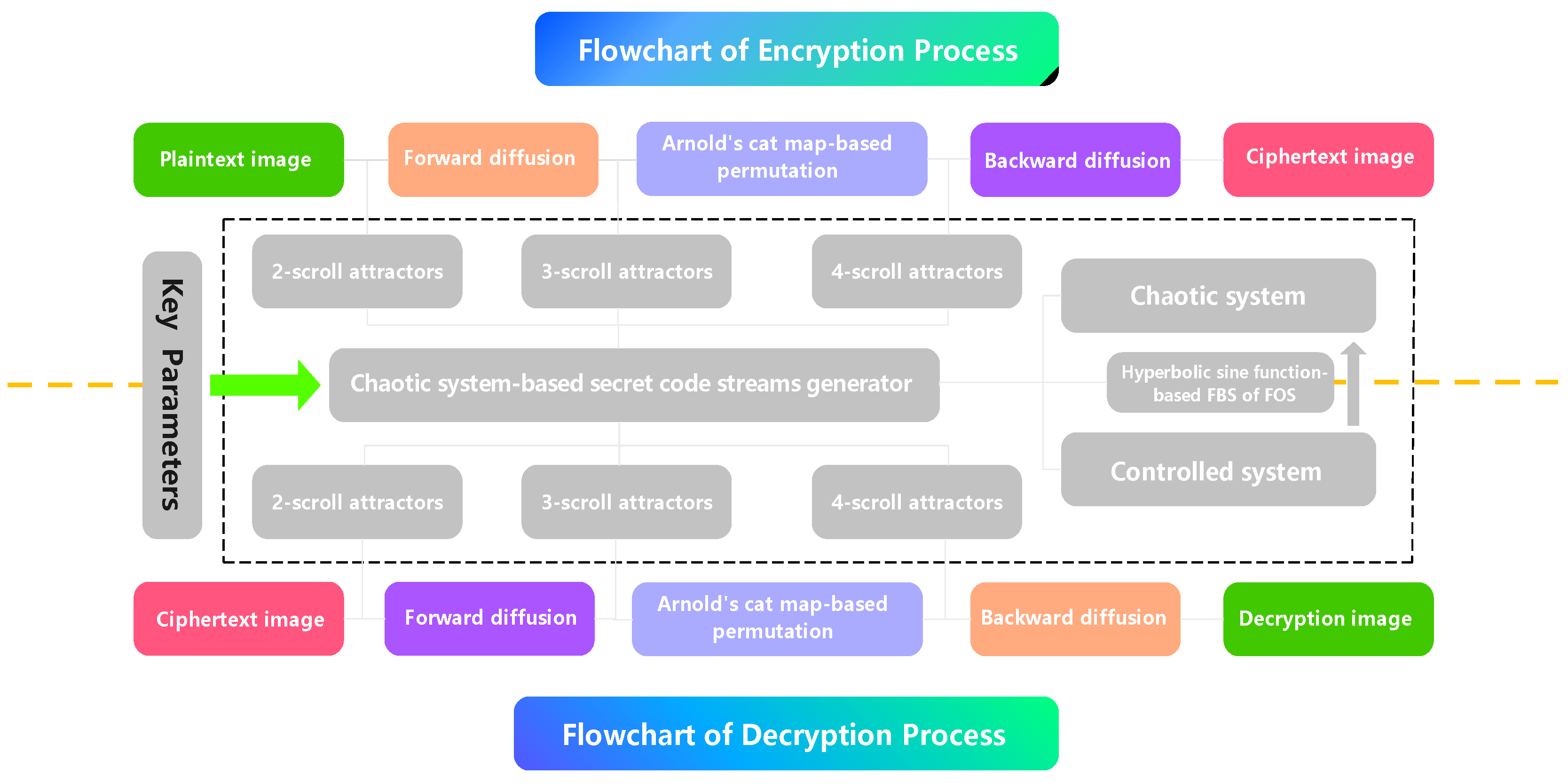
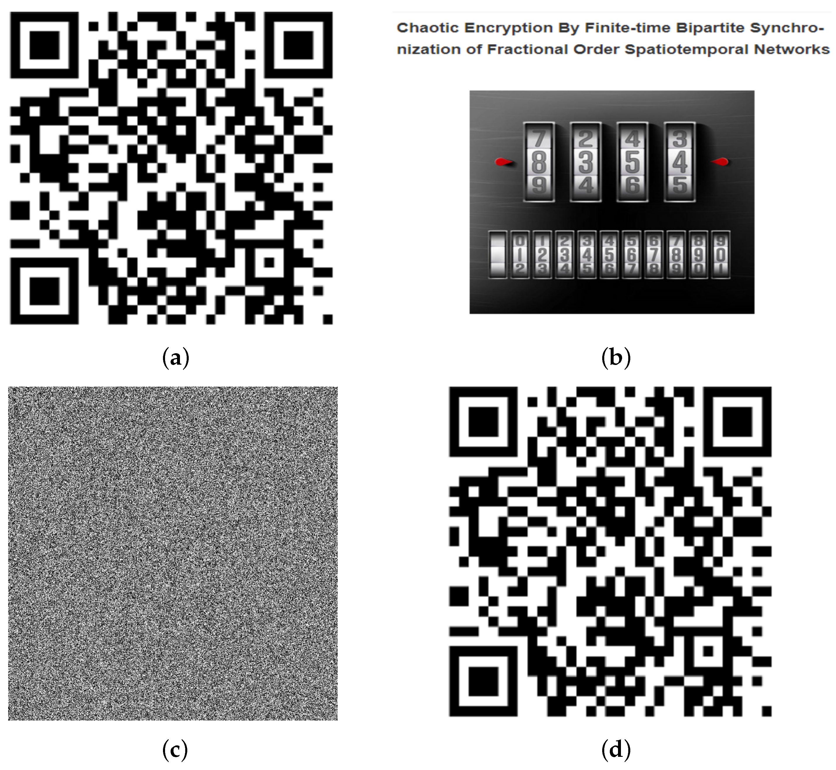
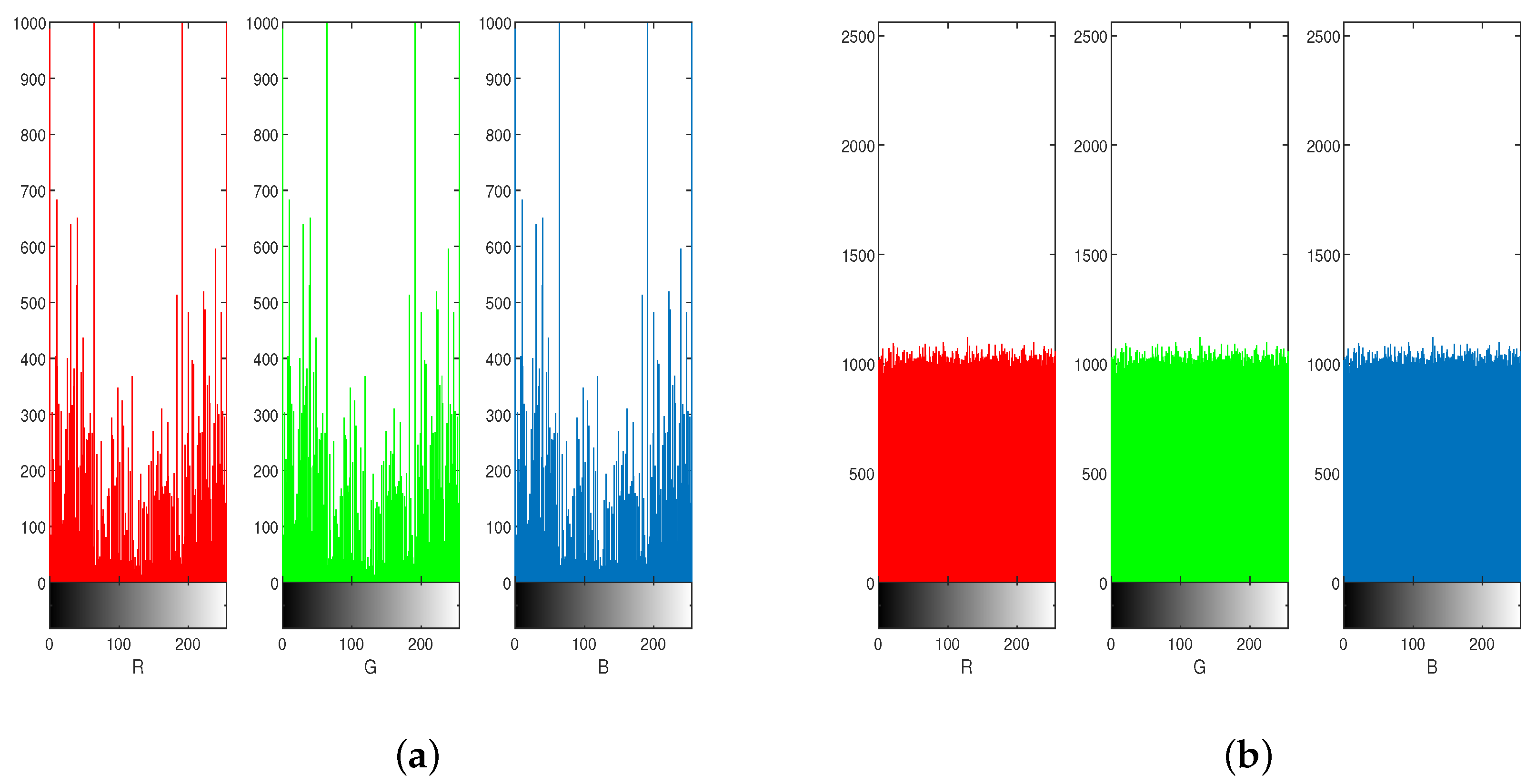
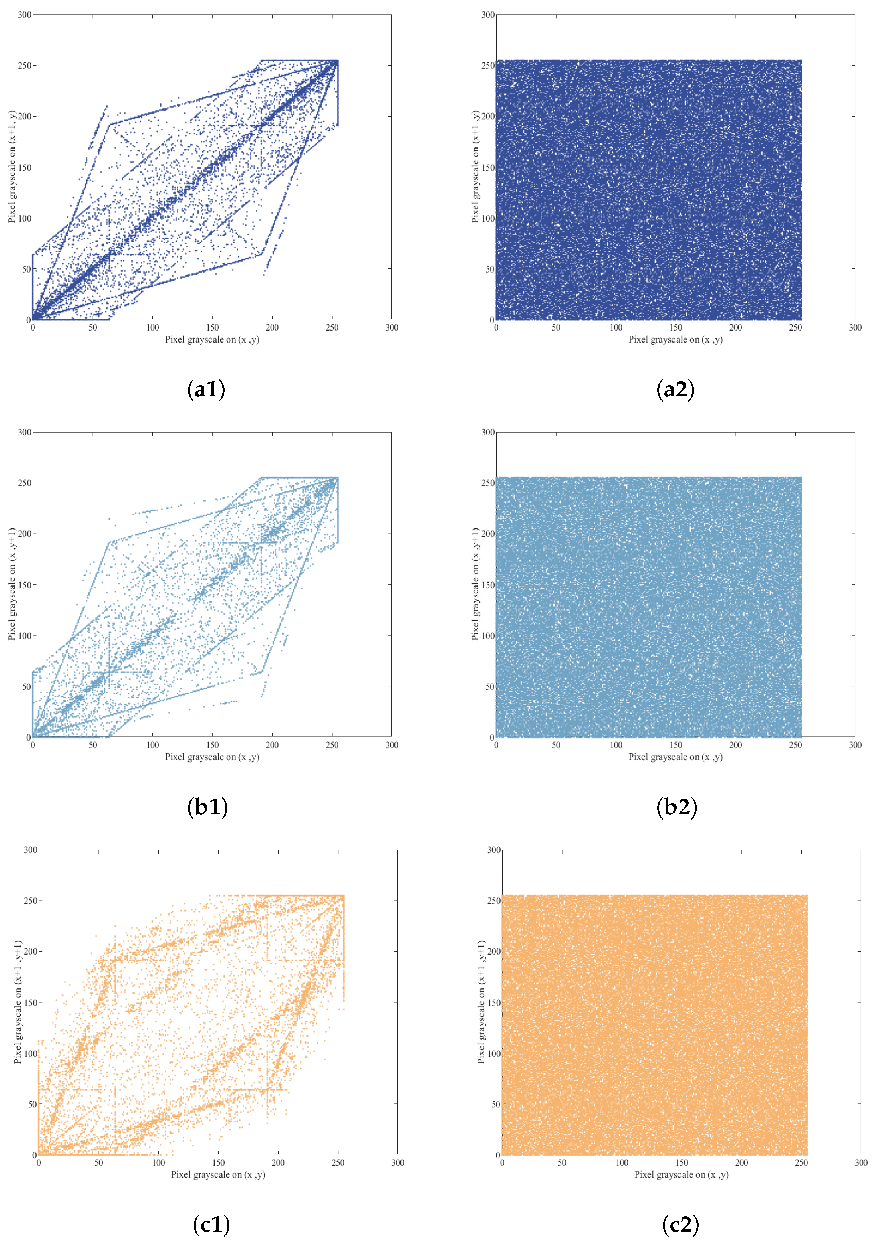
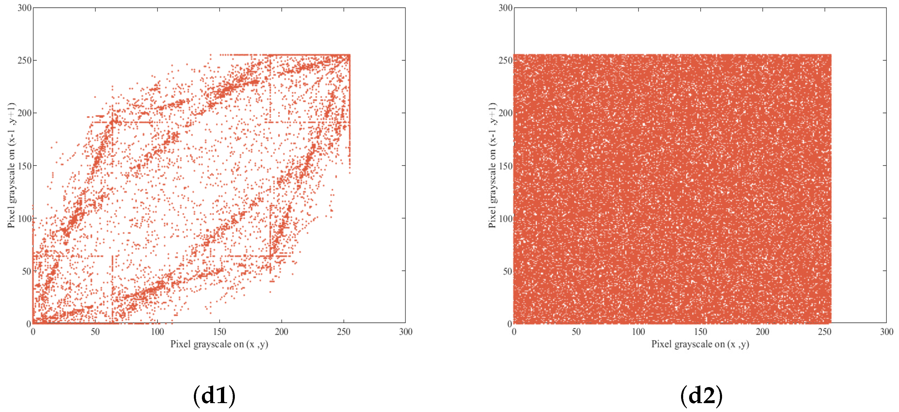
The work is organized as follows. Section 2 provides some necessary preliminaries and the model description. In Section 3, the HSF control is considered via a comparative analysis with two additional specific control protocols. Some simulations are carried out to support our findings in Section 4. In Section 5, the  application of our results in image encryption is presented.

Notations. Denote $\mathcal{N}=\{1,2,\dots ,N\}$ and $\overline{n}=\{1,2,\dots ,n\}$. Let $\mathbb{R},{\mathbb{R}}^n$, and ${\mathbb{R}}^{n\times m}$ represent the space of real numbers, the n-dimensional Euclidean space, and the $n\times m$ real matrices, respectively. ${\mathbb{R}}^{+}=[0,+\infty )$. ${\mathbb{Z}}^{+}$ is the set of all positive integers. $\mathrm{diag}\{·\}$ represents the diagonal matrix. ⊗, ${\mathbf{0}}_m$, and $1_m$ denote the Kronecker product, column vector with all zero elements, and column vector with of all ones, respectively. For any $Z\in {\mathbb{R}}^{n\times n}$, $Z^T$ and $Z\le 0$ signify the transposition of matrix Z and negative semi-definite matrix Z, respectively: $\parallel Z\parallel =\sqrt{{\lambda }_{\max }\left(Z^{T}Z\right)}$, ${\left[Z\right]}^s=\frac{Z+Z^T}{2}$. For the symmetric matrix Z, ${\lambda }_{\max }\left(Z\right)$ is the maximum eigenvalue. For any $Y\in {\mathbb{R}}^n$, $\parallel Y\parallel =\sqrt{Y^{T}Y}$. ∘ denotes the Hadamard product:  $A={\left(a_{ij}\right)}_{n\times m}$; $B={\left(b_{ij}\right)}_{n\times m}$; $A\circ B={(a_{ij}·b_{ij})}_{n\times m}$.vec(·) symbolizes the straightening operation.

2. Preliminaries and Model Description

In this section, some essential definitions, lemmas, and assumptions are presented, along with the model description.

Definition 1 

([36]). The fractional-order Caputo derivative of $F\left(t\right)\in C^1\left({\mathbb{R}}^{+},\mathbb{R}\right)$ is defined by

$$\begin{array}{c}\hfill {}_{t_0}{}^{C}D_t^{\alpha }F\left(t\right)=\frac{1}{\Gamma (1-\alpha )}{\int }_{t_0}^t{(t-s)}^{-\alpha }\dot{F}\left(s\right)\mathrm{d}s.\end{array}$$

(1)

Let $Q(x,t):\Omega \times {\mathbb{R}}^{+}\to \mathbb{R}$ be derivable with regard to t and  $\alpha \in (0,1)$.

Definition 2 

([36]). The fractional-order Caputo derivative of continuous differentiable function $Q(x,t)$ with regard to t is defined by

$$\begin{array}{c}\hfill \frac{{\partial }^{\alpha }Q(x,t)}{\partial t^{\alpha }}=\frac{1}{\Gamma (1-\alpha )}{\int }_{t_0}^t\frac{\partial Q(x,s)}{\partial s}{(t-s)}^{-\alpha }\mathrm{d}s.\end{array}$$

(2)

Definition 3 

([37]). A signed graph $\mathcal{G}=(\mathcal{V},\mathcal{E},\mathcal{A})$ is structurally balanced if it has a bipartite division of nodes, ${\overline{\mathcal{V}}}_1\in \mathcal{V}$ and ${\overline{\mathcal{V}}}_2\in \mathcal{V}$ such that ${\overline{\mathcal{V}}}_1\cup {\overline{\mathcal{V}}}_2=\mathcal{V},{\overline{\mathcal{V}}}_1\cap {\overline{\mathcal{V}}}_2=\varnothing$ and ${\mathcal{A}}_{ij}\ge 0,\forall i,j\in {\overline{\mathcal{V}}}_q(q\in \{1,2\}),{\mathcal{A}}_{ij}\le 0,\forall i\in {\overline{\mathcal{V}}}_p,j\in {\overline{\mathcal{V}}}_r,p\ne$$r(p,r\in \{1,2\left\}\right)$.

Assumption 1. 

The topology graph $\mathcal{G}$ of the addressed network is strongly connected and structurally balanced.

Assumption 2. 

For nonlinear function $f(·)$: ${\mathbb{R}}^n\to {\mathbb{R}}^n$, there exists a positive constant $\vartheta >0$ such that for any vectors $y_1,y_2\in {\mathbb{R}}^n$,

$$∥f\left(y_1\right)-f\left(y_2\right)∥\le \vartheta ∥y_1-y_2∥.$$

Lemma 1 

([36]). According to the properties of $Q(x,t)$,

$$\begin{array}{c}\hfill \frac{{\partial }^{\alpha }{Q}^T(x,t)Q(x,t)}{\partial t^{\alpha }}⩽2Q^T(x,t)\frac{{\partial }^{\alpha }Q(t,x)}{\partial t^{\alpha }}.\end{array}$$

(3)

Lemma 2 

([36]). According to the properties of $Q(x,t)$, suppose that $Q(x,t)$ is integrable with regard to Ω. Let

$$\tilde{Q}\left(t\right)={\int }_{\Omega }Q(x,t)\mathrm{d}x,$$

then,

$$\begin{array}{c}\hfill {}_0{}^{C}D_t^{\alpha }\tilde{Q}\left(t\right)={\int }_{\Omega }\frac{{\partial }^{\alpha }Q(x,t)}{\partial t^{\alpha }}\mathrm{d}x.\end{array}$$

(4)

Lemma 3 

([30]). (Wirtinger inequality) Suppose that $W\left(x\right):\left[L_1,L_2\right]\to {\mathbb{R}}^n$ is a continuous and square integrable function satisfying  $W\left(L_1\right)={\mathbf{0}}_n$ or $W\left(L_2\right)={\mathbf{0}}_n$; then,

$$\begin{array}{c}\hfill {\int }_{L_1}^{L_2}{W}^T\left(x\right)SW\left(x\right)\mathrm{d}x\le \frac{4{\left(L_2-L_1\right)}^2}{{\pi }^2}{\int }_{L_1}^{L_2}{\left(\frac{\partial W\left(x\right)}{\partial x}\right)}^{T}S\frac{\partial W\left(x\right)}{\partial x}\mathrm{d}x.\end{array}$$

(5)

Lemma 4 

([38]). (Generalized Gauss–Ostrogradskii Theorem) Suppose that Ω is a bounded closed region with a piecewise-smooth boundary surface $\partial \Omega$ and $g\left(x\right)=\left(g_1\left(x\right),g_2\left(x\right),\dots ,g_n\left(x\right)\right), g_i\left(x\right)$$\in C^1(\Omega )$,  $i=1,2,\dots ,n$; then,

$$\underset{q}{\underbrace{{\int ...\int }_{\Omega }}}\nabla ·g\left(x\right)\mathrm{d}\Omega =\underset{q-1}{\underbrace{\oint \cdots {\oint }_{\partial \Omega }}}g\left(x\right)·\mathbf{n}\mathrm{d}\mathrm{S},$$

where n is a outward-pointing unit normal vector determined by the areal element of $\partial \Omega$. For convenience, the above equation is denoted as follows:

$$\begin{array}{c}\hfill {\int }_{\Omega }\nabla ·g\left(x\right)\mathrm{d}\Omega ={\oint }_{\partial \Omega }g\left(x\right)·\mathbf{n}\mathrm{d}\mathrm{S}.\end{array}$$

(6)

Lemma 5 

([39]). Suppose that function $h\left(t\right):{\mathbb{R}}^{+}\to {\mathbb{R}}^{Nn}$, and function $V\left(h\left(t\right)\right):{\mathbb{R}}^{Nn}\to {\mathbb{R}}^{+}$ is C-regular (positive definite, regular and radially unbounded) if there are constants $\sigma >0$ and $0\le \theta <1$ such that

$$\begin{array}{c}\hfill {}_0{}^{C}D_t^{\alpha }V\left(h\left(t\right)\right)\le -\sigma V^{\theta }\left(h\left(t\right)\right),h\left(t\right)\in {\mathbb{R}}^{Nn}/\left\{{\mathbf{0}}_{Nn}\right\},\end{array}$$

(7)

then, $V\left(t\right)$ converges to the origin within the ST $\chi \left(h\left(t_0\right)\right)$. The $\chi \left(h\left(t_0\right)\right)$ is estimated using the following equation:

$$\begin{array}{c}\hfill \chi \left(h\left(t_0\right)\right)\le {\left(\frac{\alpha B(\alpha ,1-\theta )\Lambda {\left(h\left(t_0\right)\right)}^{\alpha -\theta }}{\sigma }\right)}^{\frac{1}{\alpha }}.\end{array}$$

(8)

Remark 1. 

Equations (1) and (2) are the fundamental definitions of fractional-order Caputo derivative and fractional-order Caputo partial derivative. Equations (3) and (4) provide the essential calculation rules for the later calculation of the Caputo derivative. Equations (5) and (6) provide the key tools needed to analyze the anisotropic diffusion term. Equation (7) presents the crucial inequality estimate for the FN convergence problem and the ST can be described using Equation (8).

Consider a kind of FOSN with N vertices, described as follows:

$$\begin{array}{cc}\hfill \frac{{\partial }^{\alpha }{m}_i(x,t)}{\partial t^{\alpha }}=& \nabla ·\left(D\circ \nabla m_i(x,t)\right)+A{m}_i\left(x,t\right)+Bf\left(m_i\left(x,t\right)\right)\hfill \\ \hfill & +g{\displaystyle \sum _{j=1}^N}\left|p_{ij}\right|\Gamma \left(\mathrm{sign}\left(p_{ij}\right)m_j\left(x,t\right)-m_i(x,t)\right)+U_i(x,t),\hfill \end{array}$$

(9)

where $i\in \mathcal{N}$, $(x,t)\in \Omega \times {\mathbb{R}}^{+}$,  $m_i\left(x,t\right)$$\in {\mathcal{R}}^n$ signifies the spatiotemporal state vector of the ith node and region $\Omega =\{x={(x_1,x_2,\dots ,x_q)}^T\in {\mathbb{R}}^q:|x_k|\le L_k,k=1,\dots ,q\}$ is an open bounded domain with a smooth boundary $\partial \Omega$. $\mathring{\Omega }$ is the interior of region $\Omega$, $\partial \Omega$ is the boundary of region  $\Omega$. ∇ represents the Hamiltonian operator. $D={\left(d_{jk}\right)}_{n\times q}$ denotes the diffusion coefficient matrix, $d_{jk}>0$. $\nabla ·\left(D\circ \nabla m_i(x,t)\right)=({\sum }_{k=1}^q\partial /\partial x_k(d_{jk}\partial m_1(x,t)/\partial x_k),{\sum }_{k=1}^q$ $\partial /\partial x_k(d_{jk}\partial m_2(x,t)/\partial x_k),\dots ,{\sum }_{k=1}^q\partial /\partial x_k(d_{jk}\partial m_n(x,t)/\partial x_k){)}^T$. $A\in {\mathbb{R}}^{n\times n}$ and $B\in {\mathbb{R}}^{n\times n}$ are the coefficient matrices. $f(·)$: ${\mathbb{R}}^n\to {\mathbb{R}}^n$ is a continuous vector function and satisfies $f\left(-m_i\left(x,t\right)\right)=-f\left(m_i\left(x,t\right)\right)$. g stands for the coupling strength. $\Gamma =\mathrm{diag}\left\{{\Gamma }_1,\dots ,{\Gamma }_n\right\}>0$ depicts the internal coupling matrix. $P={\left(p_{ij}\right)}_{N\times N}$ depicts the external coupling matrix, $p_{ij}⩾0$, where $p_{ij}\ne 0$ unless there is no direct link from node j to node i. $U_i(x,t)$ is the control protocol that is to be devised.

Remark 2. 

Compared with [7,30,31], the anisotropic diffusion is adequately taken into account in the FOSN (9) using the Hadamard product and Hamiltonian operator, and the diffusion matrix can be non-diagonal or non-square. On the one hand, the diffusion matrix characterizes the spatiotemporal diffusion phenomenon. Therefore, it is required to be diagonal in [7,30,31], indicating that the diffusion weights of each node’s state component for different spatial dimensions should all be the same. However, the above construction is relatively conservative and incompatible with typical spatiotemporal neural networks. On the other hand, if the diffusion matrix is a diagonal matrix, this implies that the number of state components for the network nodes must match the number of spatiotemporal dimensions, resulting in an extraordinary idealized model. Considering these two points, our addressed network aligns more closely with real-life scenarios.

Remark 3. 

It is noteworthy that when the diffusion matrix in FOSN (9) is diagonal, the model can transform into the one considered in [7,30,31]. When the diffusion matrix in an FOSN (9) collapses into a scalar, the model can reduce to the one discussed in [32]. When n is equal to 1 in FOSN (9), the model can revert to the version of the spatiotemporal neural network model in [33]. This proves that the network presented in this paper is more universal.

The initial condition and the Dirichlet boundary condition of FOSN (9) are derived as follows:

$$\left\{\begin{array}{c}{m}_i(x,0)=m_i^0\left(x\right),x\in \mathring{\Omega },\hfill \\ m_i(x,t)={\mathbf{0}}_n,(x,t)\in \partial \Omega \times {\mathbb{R}}^{+}.\hfill \end{array}\right.$$

(10)

The corresponding isolated orbit is provided by the following equation:

$$\begin{array}{cc}\hfill \frac{{\partial }^{\alpha }s(x,t)}{\partial t^{\alpha }}=& \nabla ·\left(D\circ \nabla s\left(x,t\right)\right)+As\left(x,t\right)+Bf\left(s\left(x,t\right)\right),\hfill \end{array}$$

(11)

where $s(x,t)\in {\mathbb{R}}^n$ represents the state vector of the isolated node. The initial condition and the Dirichlet boundary condition is shown as follows:

$$\left\{\begin{array}{c}s(x,0)=s^0\left(x\right),x\in \mathring{\Omega },\hfill \\ s(x,t)={\mathbf{0}}_n,(x,t)\in \partial \Omega \times {\mathbb{R}}^{+}.\hfill \end{array}\right.$$

(12)

As per the properties of the Laplacian matrix, the FOSN (9) can be transitioned into the following:

$$\begin{array}{cc}\hfill \frac{{\partial }^{\alpha }{m}_i(x,t)}{\partial t^{\alpha }}=& \nabla ·\left(D\circ \nabla m_i(x,t)\right)+A{m}_i\left(x,t\right)+Bf\left(m_i\left(x,t\right)\right)\hfill \\ \hfill & +g{\displaystyle \sum _{j=1}^N}{\tilde{p}}_{ij}\Gamma m_j\left(x,t\right)+U_i(x,t),\hfill \end{array}$$

(13)

where $\tilde{P}={\left({\tilde{p}}_{ij}\right)}_{N\times N},{\tilde{p}}_{ij}=p_{ij}\mathrm{for}i\ne j$, and   ${\tilde{p}}_{ii}=-{\sum }_{j=1,j\ne i}^N\left|p_{ij}\right|$.

In the light of Assumption 1, there must be a gauge transformation matrix $\Pi =\mathrm{diag}\left\{{\xi }_1,{\xi }_2,\dots ,{\xi }_N\right\}$ and ${\xi }_i\in \{1,-1\}$. Hence, $\overline{P}=\Pi \tilde{P}\Pi ={\left({\overline{p}}_{ij}\right)}_{N\times N}$, where ${\overline{p}}_{ij}={\xi }_i{\tilde{p}}_{ij}{\xi }_j=\left|p_{ij}\right|$, for  $i\ne j$ and ${\overline{p}}_{ii}=-{\sum }_{j=1,j\ne i}^N\left|p_{ij}\right|$, for  $i=j$. Therefore, the FOSN (13) can be collated as follows:

$$\begin{array}{cc}\hfill \frac{{\partial }^{\alpha }{\overline{m}}_i(x,t)}{\partial t^{\alpha }}=& \nabla ·\left(D\circ \nabla {\overline{m}}_i(x,t)\right)+A{\overline{m}}_i\left(x,t\right)+Bf\left({\overline{m}}_i\left(x,t\right)\right)\hfill \\ \hfill & +g{\displaystyle \sum _{j=1}^N}{\overline{p}}_{ij}\Gamma {\overline{m}}_j\left(x,t\right)+{\xi }_i{U}_i(x,t),\hfill \end{array}$$

(14)

where ${\overline{m}}_i\left(x,t\right)={\xi }_i{m}_i\left(x,t\right)$.

Take $M_i(x,t)={\overline{m}}_i\left(x,t\right)-s(x,t)$ for the synchronization error. Using the FOSN (14) and (11), the homologous error system can be derived as follows:

$$\begin{array}{cc}\hfill \frac{{\partial }^{\alpha }{M}_i(x,t)}{\partial t^{\alpha }}=& \nabla ·\left(D\circ \nabla M_i(x,t)\right)+A{M}_i\left(x,t\right)+Bf\left(M_i\left(x,t\right)\right)\hfill \\ \hfill & +g{\displaystyle \sum _{j=1}^N}{\overline{p}}_{ij}\Gamma M_j(x,t)+{\xi }_i{U}_i(x,t),\hfill \end{array}$$

(15)

where $\tilde{f}\left(M_i\left(x,t\right)\right)=f\left({\overline{m}}_i\left(x,t\right)\right)-f\left(m_i\left(x,t\right)\right)$. The initial condition and Dirichlet boundary condition are given by the following:

$$\left\{\begin{array}{c}{M}_i(x,0)={\overline{m}}_i^0\left(x\right)-s^0\left(x\right),x\in \mathring{\Omega },\hfill \\ M_i\left(x,t\right)={\mathbf{0}}_n,(x,t)\in \partial \Omega \times {\mathbb{R}}^{+}.\hfill \end{array}\right.$$

(16)

Let $M_i^0=M_i(x,0)$, $M^0={({\left(M_1^0\right)}^T,{\left(M_2^0\right)}^T,\dots ,{\left(M_N^0\right)}^T)}^T$, $M(x,t)=({\left(M_1(x,t)\right)}^T,{\left(M_2(x,t)\right)}^T,$$\dots ,{ \left(M_N(x,t)\right)}^T{)}^T$.

Definition 4 

([40]). The FOSN (9) and (11) are said to be FTBS provided that there is a constant $\chi \left(M^0\right)\ge 0$, such that $\underset{t\to \chi \left(M^0\right)}{lim}\left|\right|M(x,t)\left|\right|=0$, $\left|\right|M(x,t)\left|\right|\equiv 0$ for any $t\ge \chi \left(M^0\right)$. $\chi \left(M^0\right)$ is regarded as the ST.

For simplicity of representation, suppose

$M_i(x,t)=M_i={(M_{i1},M_{i2},\dots ,M_{in})}^T\in {\mathbb{R}}^n$.

$D={\left(d_{jk}\right)}_{n\times q}={\left(D_1,D_2,\dots ,D_n\right)}^T$, $D_j={\left(d_{j1},d_{j2},\dots ,d_{jq}\right)}^T$ is a column vector.

$\nabla M_i={\left(\nabla M_{i1},\nabla M_{i2},\dots ,\nabla M_{in}\right)}^T$, $\nabla M_{i1}={\left(\frac{\partial M_{i1}}{\partial x_1},\frac{\partial M_{i1}}{\partial x_2},\dots ,\frac{\partial M_{i1}}{\partial x_q}\right)}^T$.

$H={(H_1^T,H_2^T,\dots ,H_n^T)}^T\in {\mathbb{R}}^{n\times q}$, $H_i\in {\mathbb{R}}^{1\times q}$ is a row vector.

$\nabla ·H={\left(\nabla ·H_1,\nabla ·H_2,\dots ,\nabla ·H_n\right)}^T$, $\nabla ·H_i=\frac{\partial H_{i1}}{\partial x_1}+\frac{\partial H_{i2}}{\partial x_2}+\dots +\frac{\partial H_{iq}}{\partial x_q}$.

Lemma 6. 

For  $M_i\in {\mathbb{R}}^n$, the following equation transformation is satisfied:

$$\begin{array}{cc}\hfill & M_i^T\left[\nabla ·\left(D\circ \nabla M_i\right)\right]=\nabla ·\left[M_i^T(D\circ \nabla M_i)\right]-1_n^T\left[\nabla M_i\circ \left(D\circ \nabla M_i\right)\right]1_q.\hfill \end{array}$$

Proof. 

$$\begin{array}{cc}\hfill & M_i^T\left[\nabla ·\left(D\circ \nabla M_i\right)\right]\hfill \\ \hfill =& {\left(\begin{array}{c}{M}_{i1}\\ M_{i2}\\ ⋮\\ M_{in}\end{array}\right)}^T\left[\nabla ·\left(\left(\begin{array}{cccc}{d}_{11}& d_{12}& \dots & d_{1q}\\ d_{21}& d_{22}& \dots & d_{2q}\\ ⋮& ⋮& & ⋮\\ d_{n1}& d_{n2}& \dots & d_{nq}\end{array}\right)\circ \left(\begin{array}{cccc}\frac{\partial M_{i1}}{\partial x_1}& \frac{\partial M_{i1}}{\partial x_2}& \dots & \frac{\partial M_{i1}}{\partial x_q}\\ \frac{\partial M_{i2}}{\partial x_1}& \frac{\partial M_{i2}}{\partial x_2}& \dots & \frac{\partial M_{i2}}{\partial x_q}\\ ⋮& ⋮& & ⋮\\ \frac{\partial M_{in}}{\partial x_1}& \frac{\partial M_{in}}{\partial x_2}& \dots & \frac{\partial M_{in}}{\partial x_q}\end{array}\right)\right)\right]\hfill \\ \hfill =& {\left(\begin{array}{c}{M}_{i1}\\ M_{i2}\\ ⋮\\ M_{in}\end{array}\right)}^T\left[\nabla ·\left(\begin{array}{cccc}{d}_{11}\frac{\partial M_{i1}}{\partial x_1}& d_{12}\frac{\partial M_{i1}}{\partial x_2}& \dots & d_{1q}\frac{\partial M_{i1}}{\partial x_q}\\ d_{21}\frac{\partial M_{i2}}{\partial x_1}& d_{22}\frac{\partial M_{i2}}{\partial x_2}& \dots & d_{2q}\frac{\partial M_{i2}}{\partial x_q}\\ ⋮& ⋮& & ⋮\\ d_{n1}\frac{\partial M_{in}}{\partial x_1}& d_{n2}\frac{\partial M_{in}}{\partial x_2}& \dots & d_{nq}\frac{\partial M_{in}}{\partial x_q}\end{array}\right)\right]\hfill \\ \hfill =& {\left(\begin{array}{c}{M}_{i1}\\ M_{i2}\\ ⋮\\ M_{in}\end{array}\right)}^T\left(\begin{array}{cccc}\nabla ·\left(d_{11}\frac{\partial M_{i1}}{\partial x_1}\right.& d_{12}\frac{\partial M_{i1}}{\partial x_2}& \dots & \left.d_{1q}\frac{\partial M_{i1}}{\partial x_q}\right)\\ \nabla ·\left(d_{21}\frac{\partial M_{i2}}{\partial x_1}\right.& d_{22}\frac{\partial M_{i2}}{\partial x_2}& \dots & \left.d_{2q}\frac{\partial M_{i2}}{\partial x_q}\right)\\ & ⋮\\ \nabla ·\left(d_{n1}\frac{\partial M_{in}}{\partial x_1}\right.& d_{n2}\frac{\partial M_{in}}{\partial x_2}& \dots & \left.d_{nq}\frac{\partial M_{in}}{\partial x_q}\right)\end{array}\right)\hfill \\ \hfill =& {\left(\begin{array}{c}{M}_{i1}\\ M_{i2}\\ ⋮\\ M_{in}\end{array}\right)}^T\left(\begin{array}{c}{\displaystyle \sum _{k=1}^q}{d}_{1k}\frac{{\partial }^2{M}_{i1}}{\partial x_k^2}\\ {\displaystyle \sum _{k=1}^q}{d}_{2k}\frac{{\partial }^2{M}_{i2}}{\partial x_k^2}\\ ⋮\\ {\displaystyle \sum _{k=1}^q}{d}_{nk}\frac{{\partial }^2{M}_{in}}{\partial x_k^2}\end{array}\right)\hfill \\ \hfill =& {\displaystyle \sum _{j=1}^n}{\displaystyle \sum _{k=1}^q}{d}_{jk}{M}_{ij}\frac{{\partial }^2{M}_{ij}}{\partial x_k^2}={\displaystyle \sum _{j=1}^n}{\displaystyle \sum _{k=1}^q}{d}_{jk}\left[\frac{\partial \left(M_{ij}\frac{\partial M_{ij}}{\partial x_k}\right)}{\partial x_k}-{\left(\frac{\partial M_{ij}}{\partial x_k}\right)}^2\right]\hfill \\ \hfill =& {\displaystyle \sum _{j=1}^n}{\displaystyle \sum _{k=1}^q}{d}_{jk}\frac{\partial \left(M_{ij}\frac{\partial M_{ij}}{\partial x_k}\right)}{\partial x_k}-{\displaystyle \sum _{j=1}^n}{\displaystyle \sum _{k=1}^q}{d}_{jk}{\left(\frac{\partial M_{ij}}{\partial x_k}\right)}^2.\hfill \end{array}$$

(17)

Moreover,

$$\begin{array}{cc}\hfill {\displaystyle \sum _{j=1}^n}{\displaystyle \sum _{k=1}^q}{d}_{jk}\frac{\partial \left(M_{ij}\frac{\partial M_{ij}}{\partial x_k}\right)}{\partial x_k}=& \nabla ·\left({\displaystyle \sum _{j=1}^n}{d}_{j1}{M}_{ij}\frac{\partial M_{ij}}{\partial x_1},{\displaystyle \sum _{j=1}^n}{d}_{j2}{M}_{ij}\frac{\partial M_{ij}}{\partial x_2},\dots ,{\displaystyle \sum _{j=1}^n}{d}_{jq}{M}_{ij}\frac{\partial M_{ij}}{\partial x_q}\right)\hfill \\ \hfill =& \nabla ·\left[{\left(\begin{array}{c}{M}_{i1}\\ M_{i2}\\ ⋮\\ M_{in}\end{array}\right)}^T\left(\begin{array}{cccc}{d}_{11}\frac{\partial M_{i1}}{\partial x_1}& d_{12}\frac{\partial M_{i1}}{\partial x_2}& \dots & d_{1q}\frac{\partial M_{i1}}{\partial x_q}\\ d_{21}\frac{\partial M_{i2}}{\partial x_1}& d_{22}\frac{\partial M_{i2}}{\partial x_2}& \dots & d_{2q}\frac{\partial M_{i2}}{\partial x_q}\\ ⋮& ⋮& & ⋮\\ d_{n1}\frac{\partial M_{in}}{\partial x_1}& d_{n2}\frac{\partial M_{in}}{\partial x_2}& \dots & d_{nq}\frac{\partial M_{in}}{\partial x_q}\end{array}\right)\right]\hfill \\ \hfill =& \nabla ·\left[M_i^T(D\circ \nabla M_i)\right],\hfill \end{array}$$

(18)

$$\begin{array}{cc}\hfill {\displaystyle \sum _{j=1}^n}{\displaystyle \sum _{k=1}^q}{d}_{jk}{\left(\frac{\partial M_{ij}}{\partial x_k}\right)}^2=& \left({\displaystyle \sum _{j=1}^n}{d}_{j1}{\left(\frac{\partial M_{ij}}{\partial x_1}\right)}^2,{\displaystyle \sum _{j=1}^n}{d}_{j2}{\left(\frac{\partial M_{ij}}{\partial x_2}\right)}^2,\dots ,{\displaystyle \sum _{j=1}^n}{d}_{jq}{\left(\frac{\partial M_{ij}}{\partial x_q}\right)}^2\right)1_q\hfill \\ \hfill =& 1_n^T\left(\begin{array}{cccc}{d}_{11}{\left(\frac{\partial M_{i1}}{\partial x_1}\right)}^2& d_{12}{\left(\frac{\partial M_{i1}}{\partial x_2}\right)}^2& \dots & d_{1q}{\left(\frac{\partial M_{i1}}{\partial x_q}\right)}^2\\ d_{21}{\left(\frac{\partial M_{i2}}{\partial x_1}\right)}^2& d_{22}{\left(\frac{\partial M_{i2}}{\partial x_2}\right)}^2& \dots & d_{2q}{\left(\frac{\partial M_{i2}}{\partial x_q}\right)}^2\\ ⋮& ⋮& & ⋮\\ d_{n1}{\left(\frac{\partial M_{in}}{\partial x_1}\right)}^2& d_{n2}{\left(\frac{\partial M_{in}}{\partial x_2}\right)}^2& \dots & d_{nq}{\left(\frac{\partial M_{in}}{\partial x_q}\right)}^2\end{array}\right)1_q\hfill \\ \hfill =& 1_n^T\left[\left(\begin{array}{cccc}{d}_{11}& d_{12}& \dots & d_{1q}\\ d_{11}& d_{22}& \dots & d_{2q}\\ ⋮& ⋮& & ⋮\\ d_{11}& d_{12}& \dots & d_{nq}\end{array}\right)\right.\circ \left(\begin{array}{cccc}\frac{\partial M_{11}}{\partial x_1}& \frac{\partial M_{i1}}{\partial x_2}& \dots & \frac{\partial M_{i1}}{\partial x_q}\\ \frac{\partial M_{12}}{\partial x_1}& \frac{\partial M_{i2}}{\partial x_2}& \dots & \frac{\partial M_{i2}}{\partial x_q}\\ ⋮& ⋮& & ⋮\\ \frac{\partial M_{in}}{\partial x_1}& \frac{\partial M_{in}}{\partial x_2}& \dots & \frac{\partial M_{in}}{\partial x_q}\end{array}\right)\hfill \\ \hfill & \circ \left.\left(\begin{array}{cccc}\frac{\partial M_{11}}{\partial x_1}& \frac{\partial M_{i1}}{\partial x_2}& \dots & \frac{\partial M_{i1}}{\partial x_q}\\ \frac{\partial M_{i2}}{\partial x_1}& \frac{\partial M_{i2}}{\partial x_2}& \dots & \frac{\partial M_{i2}}{\partial x_q}\\ ⋮& ⋮& & ⋮\\ \frac{\partial M_{in}}{\partial x_1}& \frac{\partial M_{in}}{\partial x_2}& \dots & \frac{\partial M_{in}}{\partial x_q}\end{array}\right)\right]1_q\hfill \\ \hfill =& 1_n^T\left(D\circ \nabla M_i\circ \nabla M_i\right)1_q\hfill \\ \hfill =& 1_n^T[\nabla M_i\circ \left(D\circ \nabla M_i\right)]1_q.\hfill \end{array}$$

(19)

From  (17)–(19), one can deduce that

$$\begin{array}{c}\hfill M_i^T\left[\nabla ·\left(D\circ \nabla M_i\right)\right]=\nabla ·\left[M_i^T(D\circ \nabla M_i)\right]-1_n^T\left[\nabla M_i\circ \left(D\circ \nabla M_i\right)\right]1_q.\end{array}$$

 □

Lemma 7. 

For  $M_i\in {\mathbb{R}}^n$, the following can be derived:

$$\begin{array}{cc}\hfill & {\displaystyle \sum _{i=1}^N}{\int }_{\Omega }{1}_n^T\left[D\circ \nabla M_i(x,t)\circ \nabla M_i(x,t)\right]1_q\mathrm{d}x\hfill \\ \hfill ⩾& \frac{{\pi }^2}{4}\underset{j,k}{\min }\left\{d_{jk}\right\}{\displaystyle \sum _{k=1}^q}\frac{1}{L_k^2}{\displaystyle \sum _{i=1}^N}{\int }_{\Omega }{M}_i^T(x,t)M_i(x,t)\mathrm{d}x.\hfill \end{array}$$

Proof. 

Based on Lemma 3 and Lemma 4,

$$\begin{array}{cc}\hfill & {\displaystyle \sum _{i=1}^N}{\int }_{\Omega }{1}_n^T\left[D\circ \nabla M_i(x,t)\circ \nabla M_i(x,t)\right]1_q\mathrm{d}x\hfill \\ \hfill ⩾& \underset{j,k}{\min }\left\{d_{jk}\right\}{\displaystyle \sum _{i=1}^N}{\int }_{\Omega }{1}_n^T\left[\nabla M_i(x,t)\circ \nabla M_i(x,t)\right]1_q\mathrm{d}x\hfill \\ \hfill =& \underset{j,k}{\min }\left\{d_{jk}\right\}{\displaystyle \sum _{i=1}^N}{\int }_{\Omega }trace\left[{\nabla }^T{M}_i\left(x,t\right)\nabla M_i\left(xt\right)\right]\mathrm{d}x\hfill \\ \hfill =& \underset{j,k}{\min }\left\{d_{jk}\right\}{\displaystyle \sum _{i=1}^N}{\int }_{\Omega }{\mathrm{vec}}^T\left(\nabla M_i(x,t)\right)\mathrm{vec}\left(\nabla M_i(x,t)\right)\mathrm{d}x\hfill \\ \hfill =& \underset{j,k}{\min }\left\{d_{jk}\right\}{\displaystyle \sum _{i=1}^N}{\int }_{\Omega }{\displaystyle \sum _{k=1}^q}{\left(\frac{\partial M_{i1}}{\partial x_k},\frac{\partial M_{i2}}{\partial x_k},\dots ,\frac{\partial M_{in}}{\partial x_k}\right)}^T\left(\frac{\partial M_{i1}}{\partial x_k},\frac{\partial M_{i2}}{\partial x_k},\dots ,\frac{\partial M_{in}}{\partial x_k}\right)\mathrm{d}x\hfill \end{array}$$

$$\begin{array}{cc}\hfill =& \underset{j,k}{\min }\left\{d_{jk}\right\}{\displaystyle \sum _{i=1}^n}{\displaystyle \sum _{k=1}^q}{\int }_{\Omega }{\left(\frac{\partial M_i(x,t)}{\partial x_k}\right)}^T\frac{\partial M_i(x,t)}{\partial x_k}\mathrm{d}x\hfill \\ \hfill ⩾& \frac{{\pi }^2}{4}\underset{j,k}{\min }\left\{d_{jk}\right\}{\displaystyle \sum _{k=1}^q}\frac{1}{L_k^2}{\displaystyle \sum _{i=1}^N}{\int }_{\Omega }{M}_i^T(x,t)M_i(x,t)\mathrm{d}x.\hfill \end{array}$$

 □

Remark 4. 

Compared to the studies in [7,30,31] concerning spatiotemporal networks with a diagonal diffusion matrix, Lemma 6 establishes an equality transformation for the anisotropic diffusion term, employing the vector’s inner product, the Hadamard product, and the Hamiltonian operator. Based on the matrix–vector relations, this equation transformation reveals a more concise structure and highlights a more integrated understanding of the anisotropic diffusion term at the vector level, facilitating further research into the complex dynamic behaviors of SNs.

Remark 5. 

Based on the trace results, vector straightening operation, Hadamard product, and Hamiltonian operator, Lemma 7 establishes an inequality estimate involving the anisotropic diffusion term in an effective and more compact form, which serves as the basis for the synchronization analysis later.

Remark 6. 

Notably, when the anisotropic diffusion matrix is diagonal, the conclusions of Lemmas 6 and 7 are in accordance with those in [7,30,31]. In addition, if the anisotropic diffusion matrix becomes a scalar, the results of Lemmas 6 and 7 also match the ones in [32]. More importantly, if  $n=1$, Lemmas 6 and 7 are compatible with the results for the spatiotemporal neural network model in [33], demonstrating the broader applicability of Lemmas 6 and 7.

3. Main Results

Before the detailed discussion of the designed HSF control law, the polynomial form-based control protocol and the HSF control protocol with linear terms are discussed, serving as the basic for comparison purposes.

3.1. Polynomial Form-Based Control Protocol

First, the conventional polynomial form-based control protocol was designed, as described below:

$$\begin{array}{c}\hfill U_i(x,t)=\left\{\begin{array}{cc}{\xi }_i{\overline{U}}_i(x,t),\hfill & M_i(x,t)\ne {\mathbf{0}}_n,\hfill \\ {\mathbf{0}}_n,\hfill & M_i(x,t)={\mathbf{0}}_n,\hfill \end{array}\right.\end{array}$$

(20)

where ${\overline{U}}_i(x,t)=-\phi M_i(x,t)-\psi M_i(x,t)G^{\nu }$, $G\left(t\right)={\int }_{\Omega }{M}^T(x,t)M(x,t)\mathrm{d}x$, $\phi >0,\psi >0,\nu \in (-1,0)$.

Theorem 1. 

Based on Assumptions 9 and 10 and control protocol (20), if 

$$C_1<0,$$

(21)

then FOSN (9) achieves FNBS with (11). The ST is established by

$$\chi \left(M^0\right)\le {\left(\frac{\alpha B(\alpha ,-\nu )V{\left(M^0\right)}^{\alpha -\nu -1}}{\psi }\right)}^{\frac{1}{\alpha }},$$

where  $C_1=-\frac{{\pi }^2}{4}\underset{j,k}{\min }\left\{d_{jk}\right\}{\displaystyle \sum _{k=1}^q}\frac{1}{L_k^2}+{\lambda }_{\max }\left({\left[A\right]}^s\right)+\vartheta ∥{\left[B\right]}^s∥+{\lambda }_{\max }\left(g{\left[\overline{P}\right]}^s\otimes \Gamma \right)-\phi$.

Proof. 

Construct the following Lyapunov function:

$$V\left(t\right)={\int }_{\Omega }{M}^T\left(x,t\right)M\left(x,t\right)\mathrm{d}x.$$

For $M(x,t)\in {\mathbb{R}}^{Nn}/\left\{{\mathbf{0}}_{Nn}\right\}$, in light of Lemmas 1 and 2, the following can be inferred:

$$\begin{array}{cc}\hfill {}_0{}^{C}D_t^{\alpha }V\left(t\right)⩽& 2{\int }_{\Omega }[M^T(x,t)[I_N\otimes (\nabla ·\left(D\circ \nabla M(x,t)\right))]\hfill \\ \hfill & +M^T(x,t)\left(I_N\otimes A\right)M(x,t)+M^T\left(x,t\right)\left(I_N\otimes B\right)F\left(M\left(x,t\right)\right)\hfill \\ \hfill & +g{M}^T\left(x,t\right)\left(\overline{P}\otimes \Gamma \right)M\left(x,t\right))+M^T\left(x,t\right)U(x,t)]\mathrm{d}x,\hfill \end{array}$$

(22)

where $U(x,t)={(U_1^T(x,t),U_2^T(x,t),\dots ,U_N^T(x,t))}^T$,  $F\left(M(x,t)\right)=({\tilde{f}}^T\left(M_1\left(x,t\right)\right),{\tilde{f}}^T\left(M_2\right(x,$

$t\left)\right),\dots ,{\tilde{f}}^T\left(M_N\left(x,t\right)\right){)}^T$.

Using Lemma 4 and the Dirichlet boundary condition (16), the diffusion term can be further explored as follows:

$$\begin{array}{cc}\hfill & {\int }_{\Omega }{M}^T(x,t)[I_N\otimes (\nabla ·\left(D\circ \nabla M(x,t)\right))]\mathrm{d}x\hfill \\ =\hfill & {\displaystyle \sum _{i=1}^N}{\int }_{\Omega }{M}_i^T(x,t)[\nabla ·\left(D\circ \nabla M_i(x,t)\right)]\mathrm{d}x\hfill \\ =\hfill & {\displaystyle \sum _{i=1}^N}{\int }_{\Omega }\left\{\nabla ·\left[M_i^T(x,t)(D\circ \nabla M_i(x,t))\right]-1_n^T\left[\nabla M_i(x,t)\circ \left(D\circ \nabla M_i(x,t)\right)\right]1_q\right\}\mathrm{d}x\hfill \\ =\hfill & {\displaystyle \sum _{i=1}^N}\left[{\oint }_{\partial \Omega }{M}_i^T(x,t)(D\circ \nabla M_i(x,t))·\mathbf{n}\mathrm{d}\mathrm{S}-{\int }_{\Omega }{1}_n^T\left[\nabla M_i(x,t)\circ \left(D\circ \nabla M_i(x,t)\right)\right]1_q\mathrm{d}x\right]\hfill \\ =\hfill & -{\displaystyle \sum _{i=1}^N}{\int }_{\Omega }{1}_n^T\left[\nabla M_i(x,t)\circ \left(D\circ \nabla M_i(x,t)\right)\right]1_q\mathrm{d}x.\hfill \end{array}$$

(23)

In view of Lemma 7 and (23), the following can be obtained:

$$\begin{array}{cc}\hfill & -{\displaystyle \sum _{i=1}^N}{\int }_{\Omega }{1}_n^T\left[\nabla M_i(x,t)\circ \left(D\circ \nabla M_i(x,t)\right)\right]1_q\mathrm{d}x\hfill \\ \hfill ⩽& -\frac{{\pi }^2}{4}\underset{j,k}{\min }\left\{d_{jk}\right\}{\displaystyle \sum _{k=1}^q}\frac{1}{L_k^2}{\displaystyle \sum _{i=1}^N}{\int }_{\Omega }{M}^T(x,t)M(x,t)\mathrm{d}x.\hfill \end{array}$$

(24)

Assumption 2 can be used to obtain the following:

$$\begin{array}{cc}\hfill & {\int }_{\Omega }M(x,t)\left(I_N\otimes B\right)F\left(M(x,t)\right)\mathrm{d}x\hfill \\ \hfill =& {\displaystyle \sum _{i=1}^N}{\int }_{\Omega }{M}_i^T(x,t){\left[B\right]}^s\tilde{f}\left(M_i(x,t)\right)\mathrm{d}x\hfill \\ \hfill ⩽& {\displaystyle \sum _{i=1}^N}{\int }_{\Omega }∥M_i(x,t)∥·∥{\left[B\right]}^s∥·∥\tilde{f}\left(M_i(x,t)\right)∥\mathrm{d}x\hfill \\ \hfill ⩽& {\int }_{\Omega }{M}^T(x,t)\left[I_N\otimes \left(\vartheta ∥{\left[B\right]}^s∥I_n\right)\right]M\left(x,t\right)\mathrm{d}x.\hfill \end{array}$$

(25)

Furthermore,

$$\begin{array}{cc}\hfill & {\int }_{\Omega }g{\displaystyle \sum _{i=1}^N}{M}_i^T(x,t){\displaystyle \sum _{j=1}^N}{\overline{p}}_{ij}\Gamma M_j(x,t)\mathrm{d}x\hfill \\ \hfill =& {\int }_{\Omega }g{\displaystyle \sum _{i=1}^N}{\displaystyle \sum _{k=1}^n}{M}_{ik}(x,t){\displaystyle \sum _{j=1}^N}{\overline{p}}_{ij}{\gamma }_k{M}_{jk}(x,t)\mathrm{d}x\hfill \\ \hfill =& {\int }_{\Omega }g{\displaystyle \sum _{k=1}^n}{\overline{M}}_k^T(x,t)\overline{P}{\gamma }_k{\overline{M}}_k(x,t)\mathrm{d}x\hfill \\ \hfill =& {\int }_{\Omega }{\displaystyle \sum _{k=1}^n}{\overline{M}}_k^T(x,t)g{\left[\overline{P}\right]}^s{\gamma }_k{\overline{M}}_k(x,t)\mathrm{d}x\hfill \\ \hfill ⩽& {\int }_{\Omega }{M}^T(x,t){\lambda }_{\max }\left(g{\left[\overline{P}\right]}^s\otimes \Gamma \right)M(x,t)\mathrm{d}x,\hfill \end{array}$$

(26)

where  ${\overline{M}}_k(x,t)={\left(M_{1k}(x,t),M_{2k}(x,t),\dots ,M_{Nk}(x,t)\right)}^T$. Afterwards, according to the control protocol (20),

$$\begin{array}{cc}\hfill & {\int }_{\Omega }{M}^T\left(x,t\right)U(x,t)\mathrm{d}x\hfill \\ \hfill =& {\displaystyle \sum _{i=1}^N}{\int }_{\Omega }{M}_i^T\left(x,t\right)(-\phi M_i(x,t)-\psi M_i(x,t)G^{\nu })\mathrm{d}x\hfill \\ \hfill =& -\phi V\left(t\right)-\psi V^{\nu +1}\left(t\right).\hfill \end{array}$$

(27)

Substituting (23)–(27) into (22) and homoplastically considering condition (21), one can obtain

$$\begin{array}{cc}\hfill {}_0{}^{C}D_t^{\alpha }V\left(t\right)\le & C_{1}V\left(t\right)-\psi V^{\nu +1}\left(t\right)\hfill \\ \hfill \le & -\psi V^{\nu +1}\left(t\right).\hfill \end{array}$$

(28)

According to Lemma 5, an FOSN (9) can achieve FNBS with (11). The ST is determined as follows:

$$\begin{array}{c}\hfill \chi \left(M^0\right)\le {\left(\frac{\alpha B(\alpha ,-\nu )V{\left(M^0\right)}^{\alpha -\nu -1}}{\psi }\right)}^{\frac{1}{\alpha }}.\end{array}$$

(29)

   □

3.2. HSF Control Protocol with Linear Term

Inspired by the aforementioned discussion, the result of (28) triggered us to introduce the HSF to control protocols (20), on account of its outstanding performance in [29].

Based on the conventional polynomial form-based control protocol, we introduced the HSF to explore whether it could allow for more effective control. The HSF control protocol was designed by linear terms, as follows:

$$\begin{array}{c}\hfill U_i(x,t)=\left\{\begin{array}{cc}{\xi }_i{\overline{U}}_i(x,t),\hfill & M_i(x,t)\ne {\mathbf{0}}_n,\hfill \\ {\mathbf{0}}_n,\hfill & M_i(x,t)={\mathbf{0}}_n,\hfill \end{array}\right.\end{array}$$

(30)

where ${\overline{U}}_i(x,t)=-\phi M_i(x,t)-\frac{M_i(x,t)\sinh \left(\delta G^{\sigma }\left(t\right)\right)}{G\left(t\right)}$, $\phi >0,\delta >0$,  $1>\sigma >0$.  $\sinh (·)$ is the HSF: $\sinh \left(y\right)=(e^y+e^{-y})/2$, $y\in \mathbb{R}$.

Theorem 2. 

Based on Assumptions 9 and 10 and control protocol (30), if 

$$C_1<0,$$

(31)

then the FOSN (9) achieves FNBS with (11). The ST is estimated by:

$$\chi \left(M^0\right)\le {\left(\frac{\alpha B(\alpha ,1-\sigma )V{\left(M^0\right)}^{\alpha -\sigma }}{\delta }\right)}^{\frac{1}{\alpha }},$$

where  $C_1=-\frac{{\pi }^2}{4}\underset{j,k}{\min }\left\{d_{jk}\right\}{\displaystyle \sum _{k=1}^q}\frac{1}{L_k^2}+{\lambda }_{\max }\left({\left[A\right]}^s\right)+\vartheta ∥{\left[B\right]}^s∥+{\lambda }_{\max }\left(g{\left[\overline{P}\right]}^s\otimes \Gamma \right)-\phi$.

Proof. 

Construct the following Lyapunov function:

$$\begin{array}{c}\hfill V\left(t\right)={\int }_{\Omega }{M}^T\left(x,t\right)M\left(x,t\right)\mathrm{d}x.\end{array}$$

For $M(x,t)\in {\mathbb{R}}^{Nn}/\left\{{\mathbf{0}}_{Nn}\right\}$, in light of Lemmas 1 and 2, the following can be inferred:

$$\begin{array}{cc}\hfill {}_0{}^{C}D_t^{\alpha }V\left(t\right)⩽& 2{\int }_{\Omega }[M^T(x,t)[I_N\otimes (\nabla ·\left(D\circ \nabla M(x,t)\right))]\hfill \\ \hfill & +M^T(x,t)\left(I_N\otimes A\right)M(x,t)+M^T\left(x,t\right)\left(I_N\otimes B\right)F\left(M\left(x,t\right)\right)\hfill \\ \hfill & +g{M}^T\left(x,t\right)\left(\overline{P}\otimes \Gamma \right)M\left(x,t\right))+M^T\left(x,t\right)U(x,t)]\mathrm{d}x.\hfill \end{array}$$

(32)

Following the proof process like Theorem 1, together with the control protocol (30), one can obtain the following:

$$\begin{array}{cc}\hfill {}_0{}^{C}D_t^{\alpha }V\left(t\right)\le & C_{1}V\left(t\right)-\sinh \left(\delta G^{\sigma }\left(t\right)\right)\hfill \\ \hfill \le & -{\displaystyle \sum _{r=0}^{\infty }}\frac{{\left[\delta G^{\sigma }\left(t\right)\right]}^{2r+1}}{(2r+1)!}\hfill \\ \hfill \le & -\delta G^{\sigma }\left(t\right)\hfill \\ \hfill =& -\delta V^{\sigma }\left(t\right).\hfill \end{array}$$

(33)

According to Lemma 5, the FOSN (9) achieves FNBS with (11). The ST is estimated by:

$$\begin{array}{c}\hfill \chi \left(M^0\right)\le {\left(\frac{\alpha B(\alpha ,1-\sigma )V{\left(M^0\right)}^{\alpha -\sigma }}{\delta }\right)}^{\frac{1}{\alpha }}.\end{array}$$

(34)

 □

3.3. HSF Control Law Without Linear Terms

Notably, not only can the key second power term in the devised control protocol (20) be replaced by composing the HSF with $G\left(t\right)$, but the remaining linear term, which is an important part of both control protocols (20) and (30), can also be eliminated. The HSF control law without linear terms was designed as follows:

$$\begin{array}{c}\hfill U_i(x,t)=\left\{\begin{array}{cc}{\xi }_i{\overline{U}}_i(x,t),\hfill & M_i(x,t)\ne {\mathbf{0}}_n,\hfill \\ {\mathbf{0}}_n,\hfill & M_i(x,t)={\mathbf{0}}_n,\hfill \end{array}\right.\end{array}$$

(35)

where ${\overline{U}}_i(x,t)=-\frac{M_i(x,t)\sinh \left(\delta G^{\sigma }\left(t\right)\right)}{G\left(t\right)}$, $\sigma =\frac{1}{2h+1}$, $h\in {\mathbb{Z}}^{+}$.

Theorem 3. 

Based on Assumptions 9 and 10 and control law (35), if 

$$C_2<\frac{{\delta }^{2h+1}}{(2h+1)!},$$

(36)

then the FOSN (9) achieves FNBS with (11). The ST is estimated by:

$$\chi \left(M^0\right)\le {\left(\frac{\alpha (2h-1)!B(\alpha ,\frac{2}{2h+1})V{\left(M^0\right)}^{\alpha -\frac{2h-1}{2h+1}}}{{\delta }^{2h-1}}\right)}^{\frac{1}{\alpha }},$$

where  $C_2=-\frac{{\pi }^2}{4}\underset{j,k}{\min }\left\{d_{jk}\right\}{\displaystyle \sum _{k=1}^q}\frac{1}{L_k^2}+{\lambda }_{\max }\left({\left[A\right]}^s\right)+\vartheta ∥{\left[B\right]}^s∥+{\lambda }_{\max }\left(g{\left[\overline{P}\right]}^s\otimes \Gamma \right)$.

Proof. 

Construct the following Lyapunov function:

$$\begin{array}{c}\hfill V\left(t\right)={\int }_{\Omega }{M}^T\left(x,t\right)M\left(x,t\right)\mathrm{d}x.\end{array}$$

For $M(x,t)\in {\mathbb{R}}^{Nn}/\left\{{\mathbf{0}}_{Nn}\right\}$, in light of Lemmas 1 and 2, the following can be inferred:

$$\begin{array}{cc}\hfill {}_0{}^{C}D_t^{\alpha }V\left(t\right)⩽& 2{\int }_{\Omega }[M^T(x,t)[I_N\otimes (\nabla ·\left(D\circ \nabla M(x,t)\right))]\hfill \\ \hfill & +M^T(x,t)\left(I_N\otimes A\right)M(x,t)+M^T\left(x,t\right)\left(I_N\otimes B\right)F\left(M\left(x,t\right)\right)\hfill \\ \hfill & +g{M}^T\left(x,t\right)\left(\overline{P}\otimes \Gamma \right)M\left(x,t\right))+M^T\left(x,t\right)U(x,t)]\mathrm{d}x\hfill \\ \hfill ⩽& C_{2}V\left(t\right)-\sinh \left(\delta G^{\sigma }\left(t\right)\right).\hfill \end{array}$$

(37)

Besides,

$$\begin{array}{cc}\hfill & \sinh \left(\delta G^{\sigma }\left(t\right)\right)\hfill \\ \hfill =& {\displaystyle \sum _{r=0}^{\infty }}\frac{{\left(\delta G^{\sigma }\left(t\right)\right)}^{2r+1}}{(2r+1)!}\hfill \\ \hfill =& {\displaystyle \sum _{r=0}^{h-2}}\frac{{\left(\delta G^{\sigma }\left(t\right)\right)}^{2r+1}}{(2r+1)!}+\frac{{\delta }^{2h-1}}{(2h-1)!}{G}^{\frac{2h-1}{2h+1}}\left(t\right)+\frac{{\delta }^{2h+1}}{(2h+1)!}G\left(t\right)+{\displaystyle \sum _{r=0}^{\infty }}\frac{{\left(\delta G^{\sigma }\left(t\right)\right)}^{2(r+h)+3}}{\left(2(r+h)+3\right)!}\hfill \\ \hfill \ge & \frac{{\delta }^{2h-1}}{(2h-1)!}{G}^{\frac{2h-1}{2h+1}}\left(t\right)+\frac{{\delta }^{2h+1}}{(2h+1)!}G\left(t\right).\hfill \end{array}$$

(38)

Following the proof process in Theorem 1, together with the control laws presented in (35) and (38), one can obtain

$$\begin{array}{cc}\hfill {}_0{}^{C}D_t^{\alpha }V\left(t\right)\le & \left[C_2-\frac{{\delta }^{2h+1}}{(2h+1)!}\right]V\left(t\right)-\frac{{\delta }^{2h-1}}{(2h-1)!}{V}^{\frac{2h-1}{2h+1}}\left(t\right),\hfill \\ \hfill \le & -\frac{{\delta }^{2h-1}}{(2h-1)!}{V}^{\frac{2h-1}{2h+1}}\left(t\right).\hfill \end{array}$$

(39)

According to Lemma 5, the FOSN (9) achieves FNBS with (11). The ST can be derived as follows:

$$\chi \left(M^0\right)\le {\left(\frac{\alpha (2h-1)!B(\alpha ,\frac{2}{2h+1})V{\left(M^0\right)}^{\alpha -\frac{2h-1}{2h+1}}}{{\delta }^{2h-1}}\right)}^{\frac{1}{\alpha }}.$$

 □

Remark 7. 

Differing from the designed control schemes in [29,41], the devised HSF control law (35) only has one term based on the HSF without the linear term. Actually, the linear term can ensure asymptotic synchronization, and the term based on the HSF in [29,41] is the key to ensuring synchronization in a finite time. Truthfully if FN synchronization holds, asymptotic synchronization automatically follows. Moreover, in (38), it is evidenced that the HSF can compensate the linear term by itself. Hence, the devised HSF control law (35) is more concise and further reduces the number of control parameters, facilitating easier implementation. Also, the synchronization condition (36) is less conservative and more flexible.

Remark 8. 

As opposed to the designed control schemes in [7,35], the devised HSF control law (35) does not have the sign function, which effectively avoids chattering and makes the system dynamics more smoothly. On the other hand, as a generalized exponential function, the HSF can degenerate into the standard exponential function; that is to say, the devised control law (35) can degenerete into the designed control scheme in [7,35] to some extent. In these two applications, compared with the designed control schemes in [7,35], the devised HSF control law (35) serves as not only an extension but also as an improvement, avoiding the chattering and increasing the smoothness for the control input.

Remark 9. 

As is widely recognized, in contrast to the hyperbolic cosine function, the HSF is an odd function and continuous at the origin, with the range $(-\infty ,+\infty )$. However, the range of the hyperbolic cosine function is $[1,+\infty )$, without any values in $[0,1)$. Therefore, compared to the controller with a hyperbolic cosine function in [42], the devised HSF control law (35) can provide a more flexible control input. Moreover, the control input based HSF is more smooth than the one in [42] because it does not have the sign function.

Remark 10. 

The devised HSF control law (35) can effectively control both the spatial and temporal information during the evolution of systems. To some extent, the devised control law (35) can degenerate into the control scheme in [29] through being sliced in the spatial dimension and ignoring the remaining spatial influences. This indicates that the control law we designed is more universal.

The above analysis is summarized in the following table, which shows the spatial information, linear term, sign function, and number of terms in different control laws.

References	Spatial Information	Linear Term	Sign$(·)$	Number of Terms
[29,41]	✓	✓	×	2
[7]	✓	×	✓	1
[34]	×	✓	✓	2
This work	✓	×	×	1

4. Numerical Simulations

In this section, some numerical experiments are provided to show the feasibility of the proposed control laws for FOSNs. All the simulations took place in the environment of MATLAB R2023a in Intel(R) Core(TM) i7-8750HQ CPU @2.20GHZ, a 64 bit operating system.

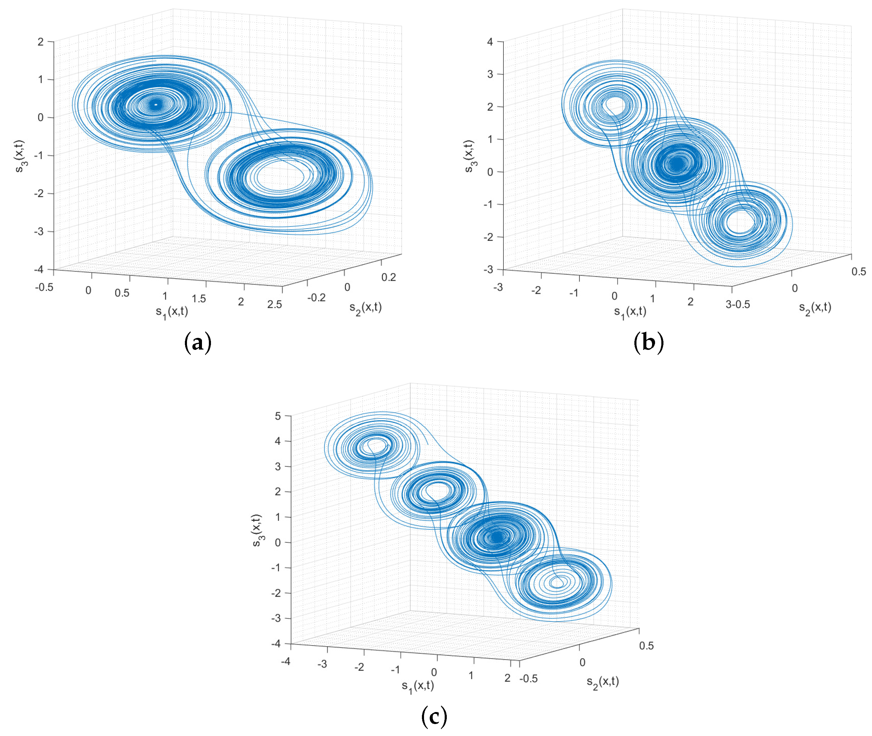
Example 1. 

Triggered by the improved Chua’s circuit in [43], the following isolated node system is established:

$$\begin{array}{cc}\hfill \frac{{\partial }^{\alpha }s(x,t)}{\partial t^{\alpha }}=& \nabla ·\left(D\circ \nabla s\left(x,t\right)\right)+As\left(x,t\right)+Bf\left(s\left(x,t\right)\right),\hfill \end{array}$$

(40)

where $s(x,t)={(s_1(x,t),s_2(x,t),s_3(x,t))}^T$, $x\in [-2,2]$

$$A=\left[\begin{array}{ccc}-0.0815\hfill & 8.8236& 0\\ 0.8159\hfill & -0.8975& 0.8159\\ 0\hfill & -11.4232& 0\end{array}\right],$$

and $B=\mathrm{diag}\left\{0.8159,0,0\right\}$,  $D=\mathrm{diag}\{0.0612,0.0612,$$0.0612\}$, $f\left(s(x,t)\right)=(f\left(s_1(x,t)\right),$  $f\left(s_2(x,t)\right),f\left(s_3(x,t)\right){)}^T$, $f\left(s_h\left(x_{,}t\right)\right)=2.1628$$sin(1.2\pi s_h(x,$  $t\left)\right)$, $h=1,2,3$. $\alpha =0.95$, $\eta =1.25$. The initial condition is $s^0\left(x\right)={(0.1,0.3,0.05)}^T$.

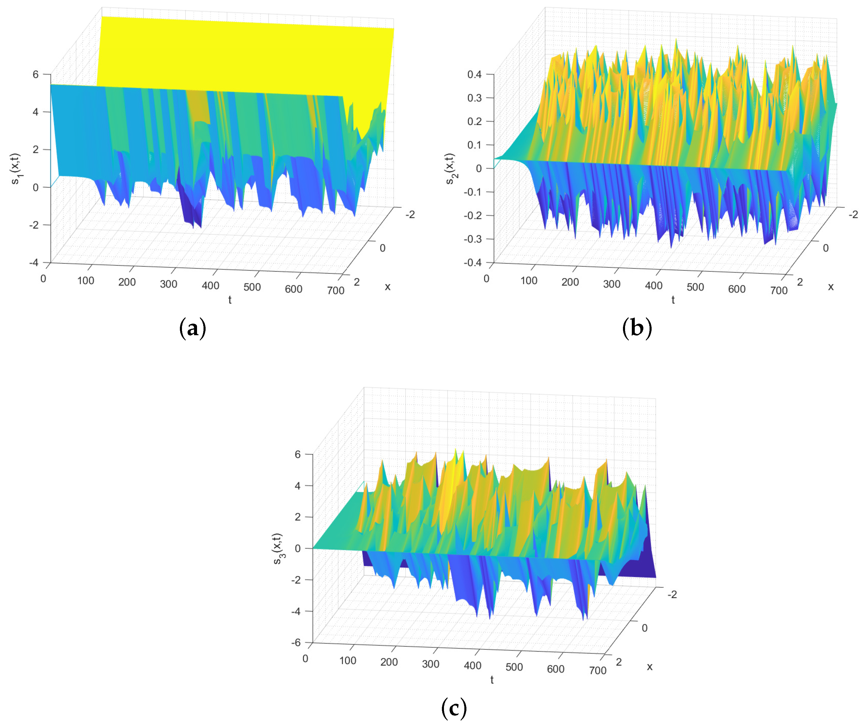
The phase portraits of $s_1(x,t)$, $s_2(x,t)$, and $s_3(x,t)$ are simulated in Figure 1. When $x=1.33$, the phase trajectory clearly has a 2-scroll chaotic attractor. When $x=-0.66$, the phase portrait clearly has a 3-scroll chaotic attractor, and when $x=0$, the phase portrait clearly has a 4-scroll chaotic attractor. It is so interesting that diverse forms of multi-scroll chaotic attractors could be generated from a deterministic system.

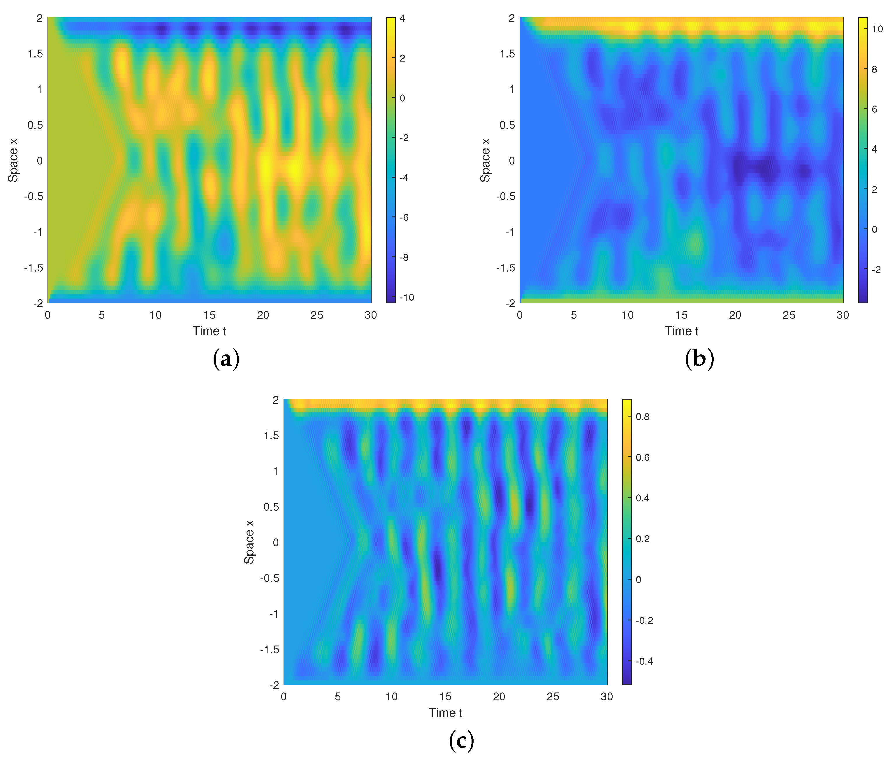
The spatiotemporal evolutions of $s_1(x,t)$, $s_2(x,t)$ and $s_3(x,t)$ are simulated in Figure 2.

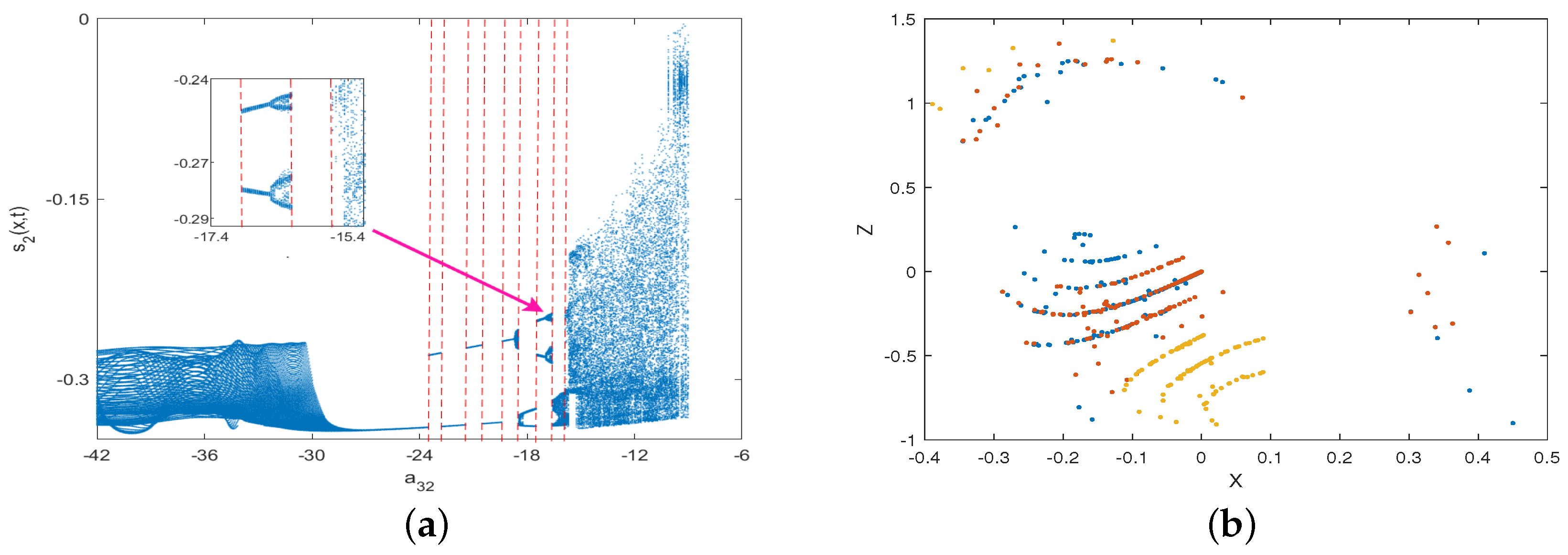
The Turing patterns of $s_1(x,t)$, $s_2(x,t)$ and $s_3(x,t)$ are simulated in Figure 3. The patterns reveal that the system (40) is Turing instability.

Figure 4a exhibits the bifurcation diagram with bifurcation parameter $a_{32}$. Following careful observation, the system state undergoes period-1 orbit, period-2 orbit, and period-4 orbit, and ultimately enters a chaotic region. Interestingly, as the system state passes through period-doubling bifurcation routed to chaos, the bifurcation diagram makes some amazing jumps, indicating that the system exhibits complex chaotic behavior. Therefore, it has better resistance to attacks in image encryption and decryption. Furthermore, it is apparent that the system falls in the chaotic region within the parameters of Example 1.

Additionally, there are some dense points with fractal structures in the Poincaré map on the plane $5x-6.1y+0.92z=0$ in Figure 4b, providing additional evidence that the system is indeed chaotic. This was the primary motivation behind our application of the theoretical results to the image encryption.

Remark 11. 

Based on the analysis of the phase portrait, spatiotemporal evolution, bifurcation diagram, Poincaré map, and Turing pattern, the established system (40) is demonstrated to be a chaotic system with strong chaos properties, which set the basis for applying the obtained synchronization results to image encryption.

Example 2. 

Consider the following FOSN, with six nodes:

$$\begin{array}{cc}\hfill \frac{{\partial }^{\alpha }{m}_i(x,t)}{\partial t^{\alpha }}=& \nabla ·\left(D\circ \nabla m_i(x,t)\right)+A{m}_i\left(x,t\right)+Bf\left(m_i\left(x,t\right)\right)\hfill \\ \hfill & +g{\displaystyle \sum _{j=1}^N}\left|p_{ij}\right|\Gamma \left(\mathrm{sign}\left(p_{ij}\right)m_j\left(x,t\right)-m_i(x,t)\right)+U_i(x,t),\hfill \end{array}$$

(41)

where  $m_i(x,t)={(m_{i1}(x,t),m_{i2}(x,t),m_{i3}(x,t))}^T$,  $\vartheta =0.1$,  $g=10$, $\Gamma =I_3$,  $i=1,2,\dots ,6$

$$P=\left[\begin{array}{cccccc}0& 0.1& 0& 0& 0& 0\\ 0& 0& 0.3& 0& -0.4& 0\\ 0& 0& 0& -0.8& 0& 0\\ 0& 0& 0& 0& 0.1& 0\\ 0& 0& 0& 0& 0& 0.6\\ -0.2& 0& 0& 0& 0& 0\end{array}\right].$$

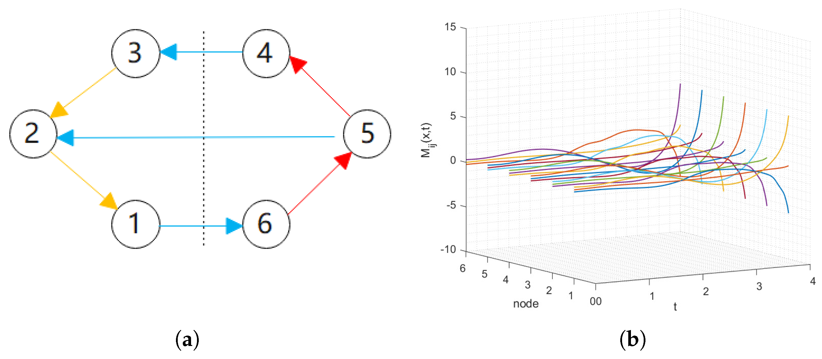
The initial condition is  $m_1^0\left(x\right)={(0.6,0.5,0.7)}^T$,  $m_2^0\left(x\right)={(0.8,0.8,0.8)}^T$,  $m_2^0\left(x\right)={(1,1.1,0.9)}^T$, $m_4^0\left(x\right)={(-1.2,-1.4,-1)}^T$,  $m_5^0\left(x\right)={(-1.4,-1.7,-1.1)}^T$,  $m_6^0\left(x\right)={(-1.6,-2,-1.15)}^T$. The network topology of FOSN (41) is depicted in Figure 5a, which indicates that the signed networks are structurally balanced with ${\overline{\mathcal{V}}}_1=\{1,2,3\}$, and ${\overline{\mathcal{V}}}_2=\{4,5,6\}$. In Figure 5a, the red lines and the yellow lines represent the cooperation relationship by positive weights and the blue lines indicate the competition relationship using negative weights, respectively.

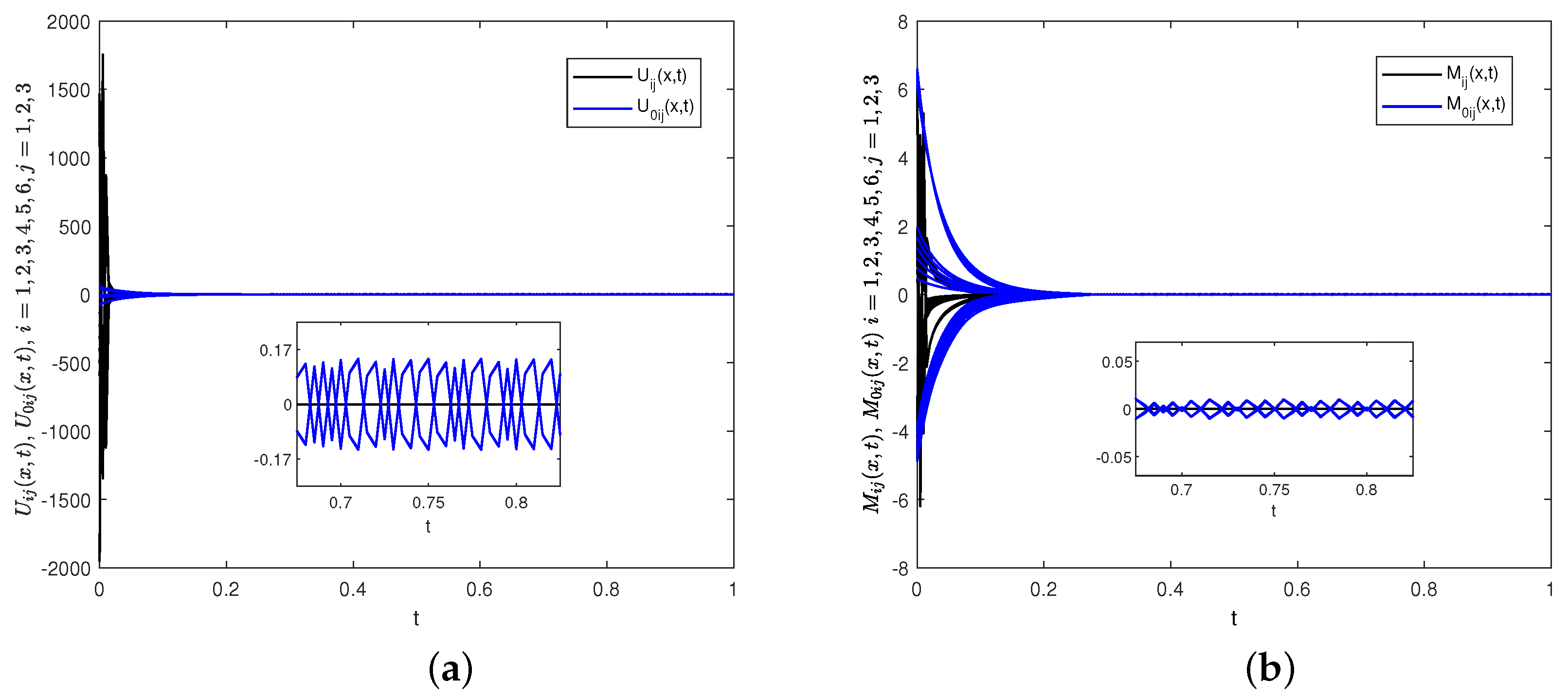
The time evolutions of $M_{ij}(x,t)$ without control are demonstrated in Figure 5b and the spatiotemporal evolutions are presented in Figure 6 with contour map, indicating that the isolated orbit is not self-stability. Figure 7 represents the states of the systems (40) with FOSN (41), signifying that they cannot achieve bipartite synchronization without control.

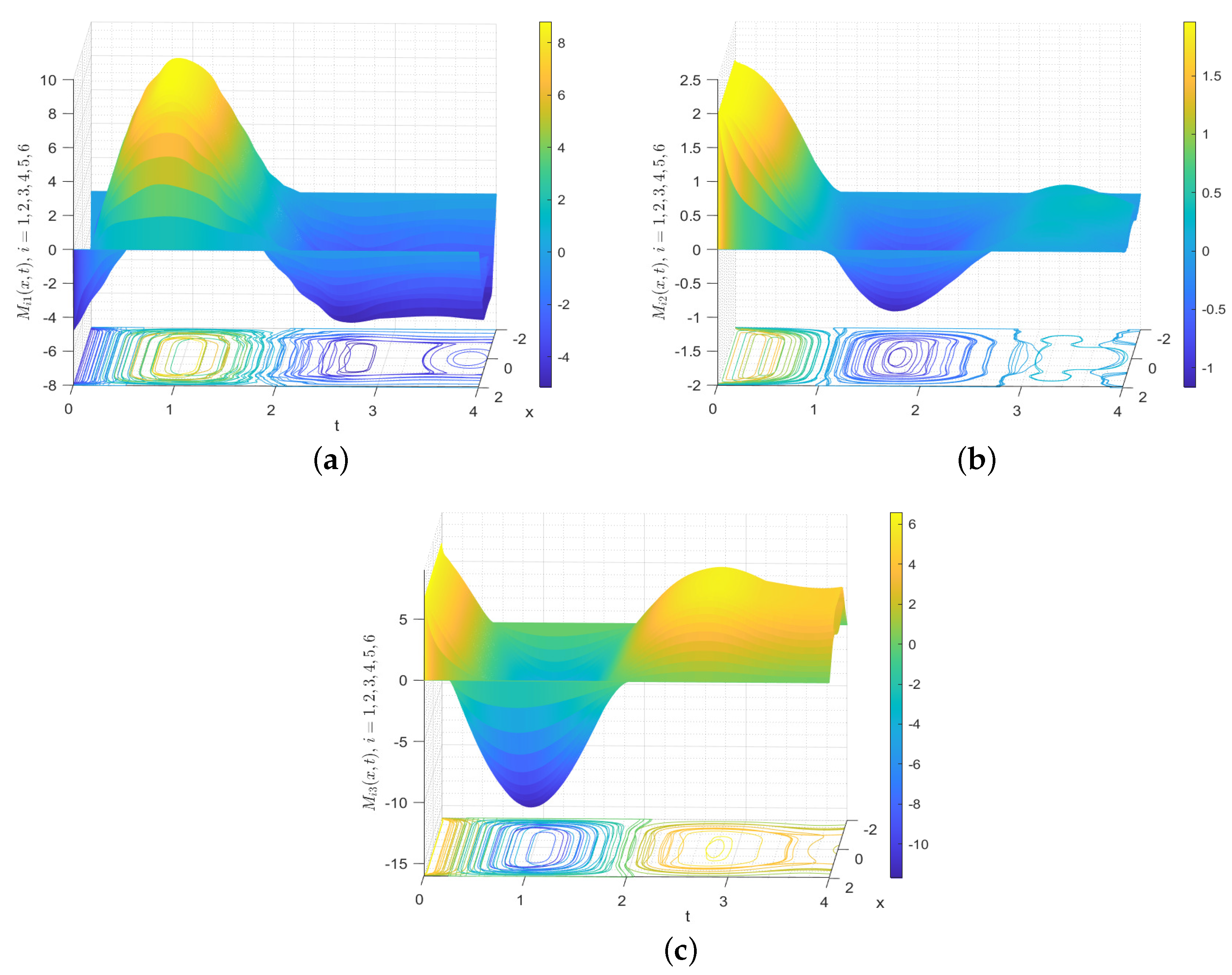
Then, the parameters of the control protocol (20) are selected as $\phi =7.49,\psi =1.5,\upsilon =-0.75$. The time evolutions of $M_{ij}(x,t)$ under the control protocol (20) are depicted in Figure 8, which show that $M_{ij}(x,t)$ gradually converges to 0 over time. Furthermore, the estimated upper bound for ST is 18.03. However, $M_{ij}(x,t)$ seems to already be very close to zero at 0.33, which indicates that the control protocol (20) deserves further investigation.

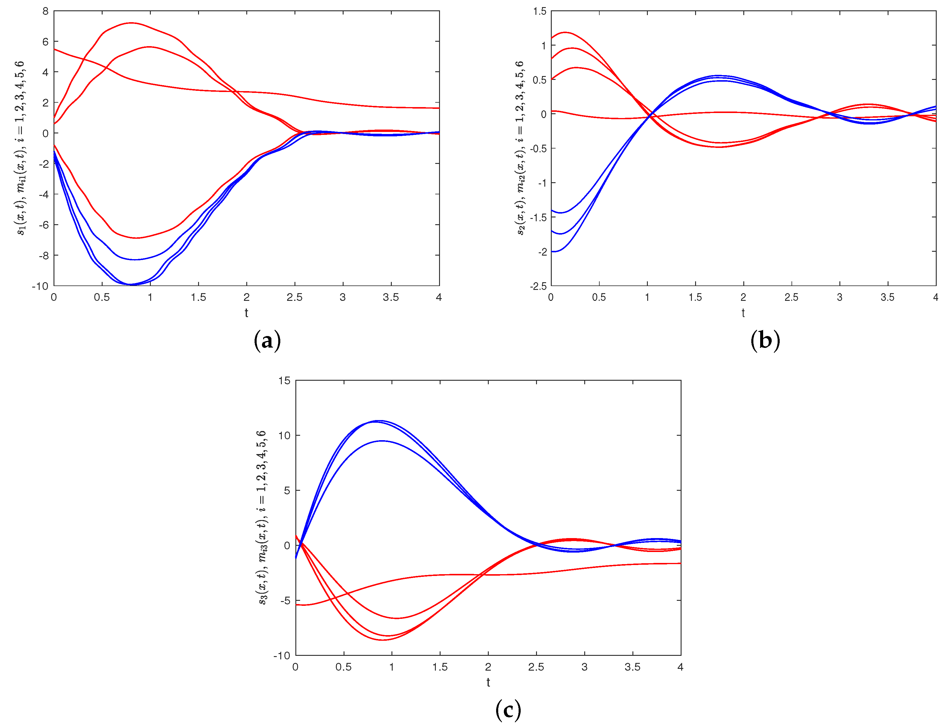
Figure 9 presents the spatiotemporal evolutions of $M_{ij}(x,t)$ with contour map, which make it clear that $M_{ij}(x,t)$ gradually converges to 0 without any alteration in height.

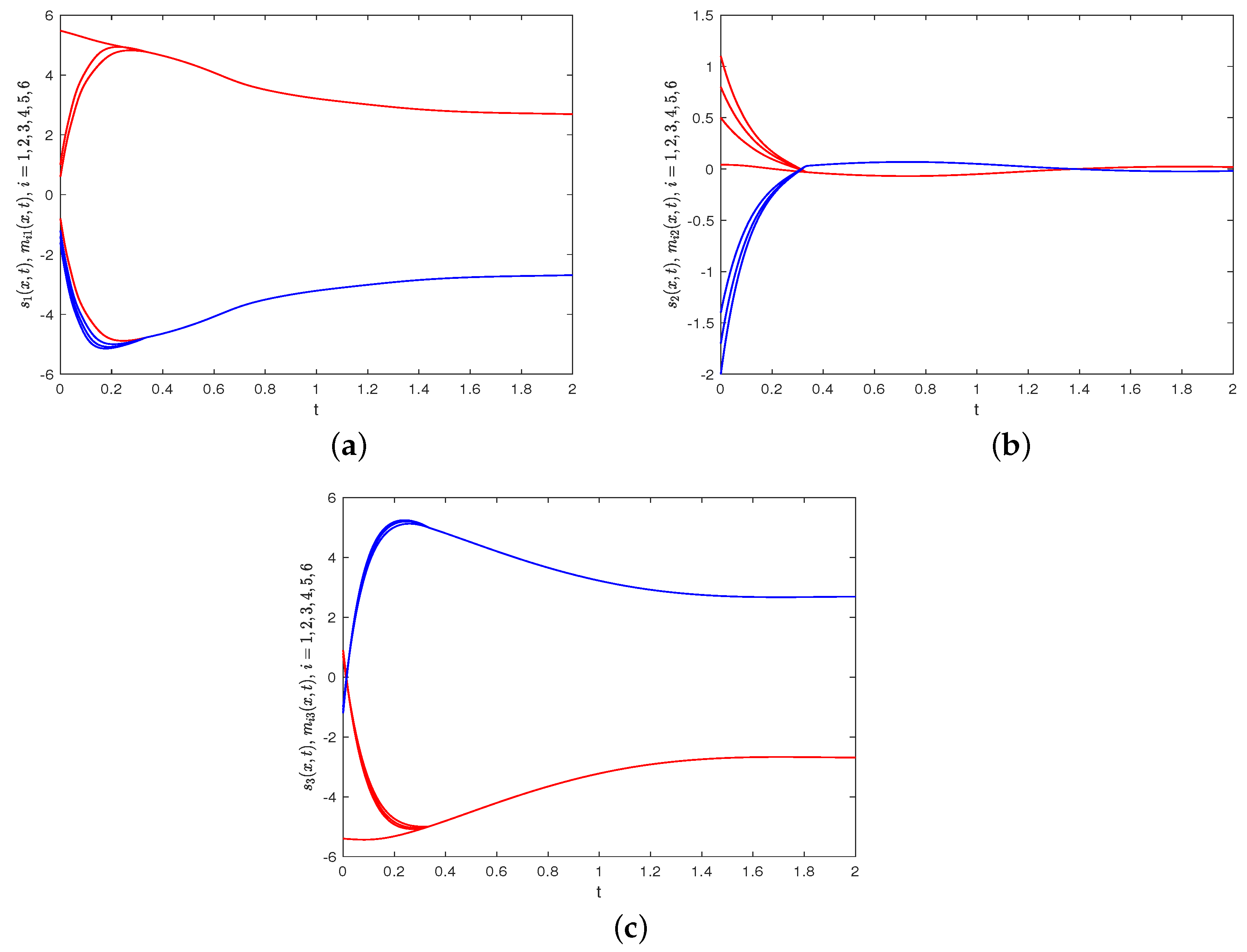
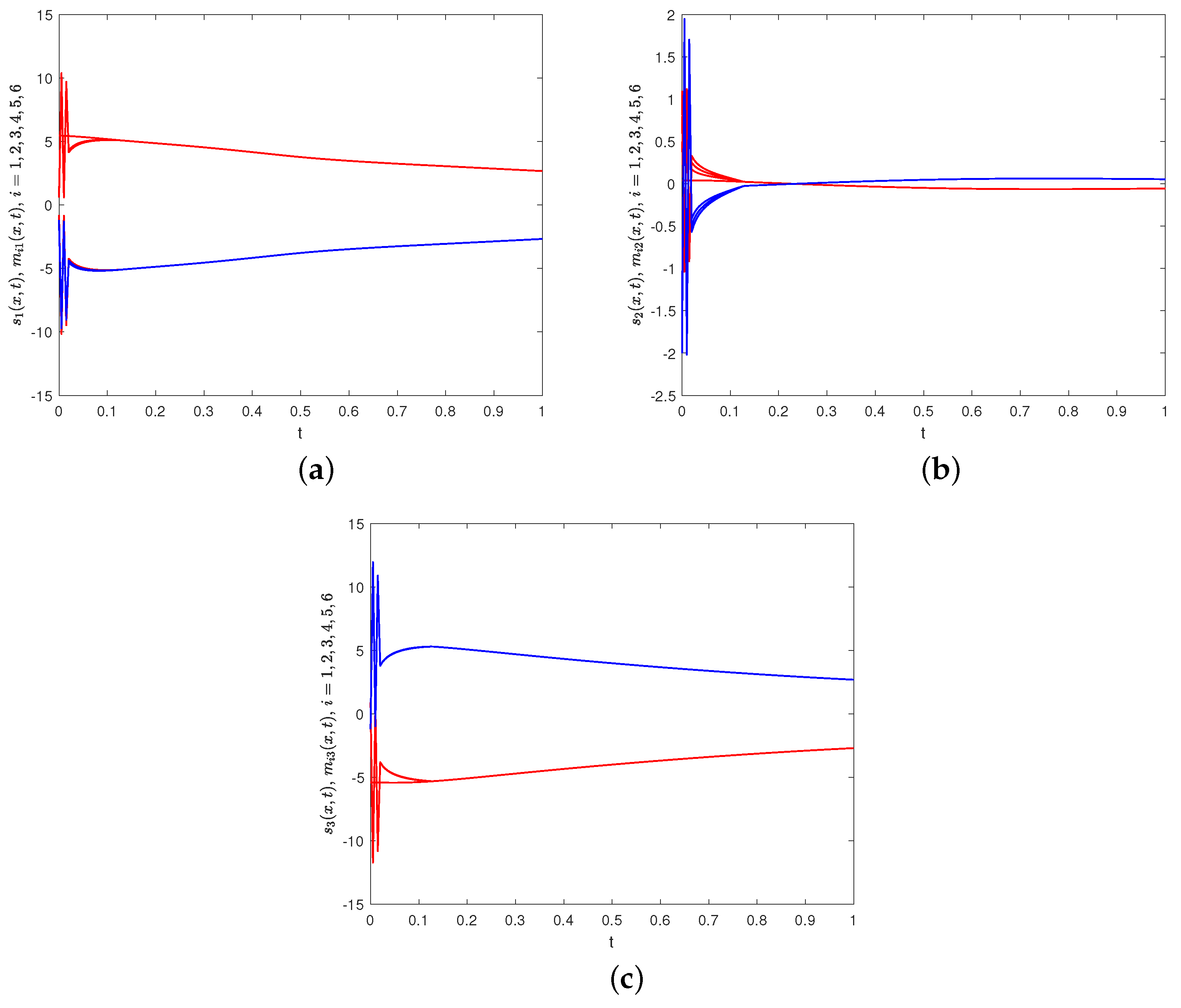
The time evolutions for each component of $m_i(x,t)$ and $s(x,t)$ are depicted in Figure 10, which indicate that the states of the network nodes in system (40) and FOSN (41) ultimately achieve BS.

Therefore, FNBS is achieved for the system (40) with FOSN (41) which verifies the correctness of the developed control protocol (20).

Example 3. 

The example will simulate system (40) with FOSN (41) under the HSF control protocol (30) with linear term in Theorem 2.

The parameters of the control protocol (30) were designed as $\phi =7.49, \delta =1.5, \sigma =0.25$ and the estimated upper bound for ST was 18.03. These parameters were selected to emphasize the excellent control performance of the HSF control protocol in comparison with this method by Algorithm 1.

Algorithm 1 Parameter selection for contrasting control protocol (20) with (30)

Input : Controlled system parameters

Output : Control parameters

START

Step 1 : Design identical control gains in linear terms for (20) and (30), meeting the conditions of (21) and (31), respectively;

Step 2 : By setting (28) equal to (33), one can obtain the following: $\delta =\psi ,\sigma =\upsilon +1$;

Step 3 : Using Step 2, one can determine the ST in (29), which is naturally equal to the result in (34) due to Lemma (5).

EXIT

The time evolutions of $M_{ij}(x,t)$ under the control protocol (30) are depicted in Figure 11, which show that $M_{ij}(x,t)$ gradually converges to 0 as time evolves. Furthermore, the estimated upper bound for ST is 18.03. However, it is worth considering that $M_{ij}(x,t)$ seems to already be very close to zero at 0.28, which indicates that the introduction of the HSF had produced positive effect.

Figure 12 describes the spatiotemporal evolutions of $M_{ij}(x,t)$ with a contour map, which make it clear that $M_{ij}(x,t)$ gradually converges to 0 in its spatiotemporal evolution without any alteration in height.

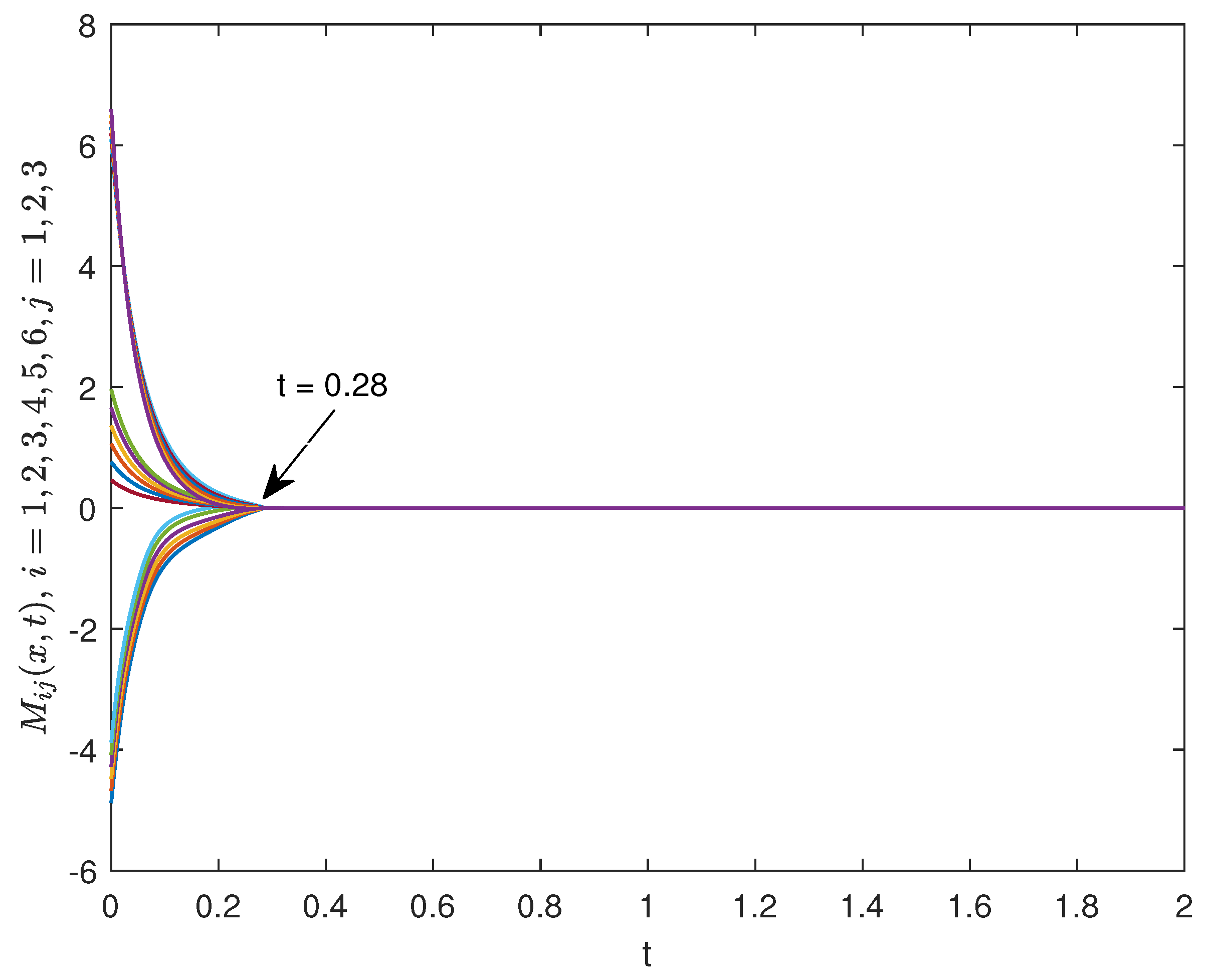
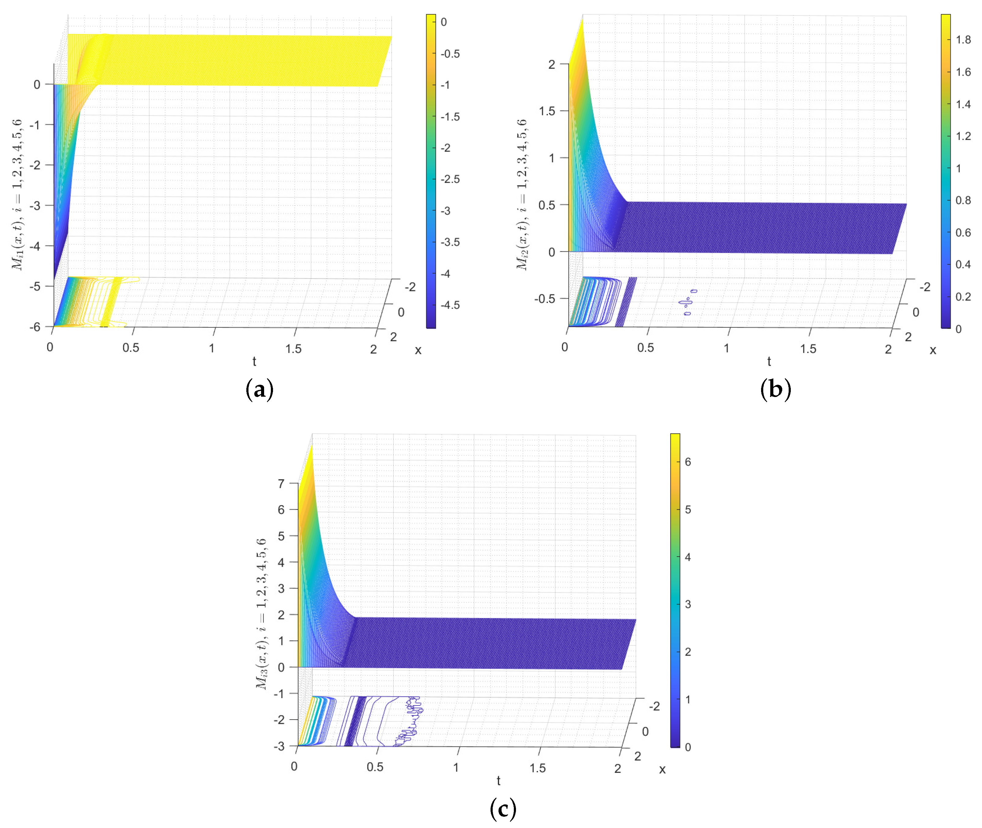
The time evolutions of each component of $m_i(x,t)$ and $s(x,t)$ are depicted in Figure 13, which show that the states of the network nodes in system (40) and FOSN (41) ultimately achieve BS.

Therefore, FNBS is achieved for the system (40) with FOSN (41), which verifies the correctness of the developed control protocol (30).

Remark 12. 

In order to make a clearer distinction between the control protocol (20) and (30), specific control parameters were selected according to Algorithm 1, guaranteeing that the estimated STs in (29) and (34) were the same. Also, the theoretical control effects were the same under the identical power-law presented in (28) and (33). As shown in Figure 8 and Figure 11, the error converges more quickly under the control protocol (30), indicating that the introduction of the HSF can reduce the convergence time and strengthen the control performance, which is tremendously significant for practical engineering applications.

Example 4. 

This example will simulate the system (40) with FOSN (41) under HSF control law without linear term in Theorem 3.

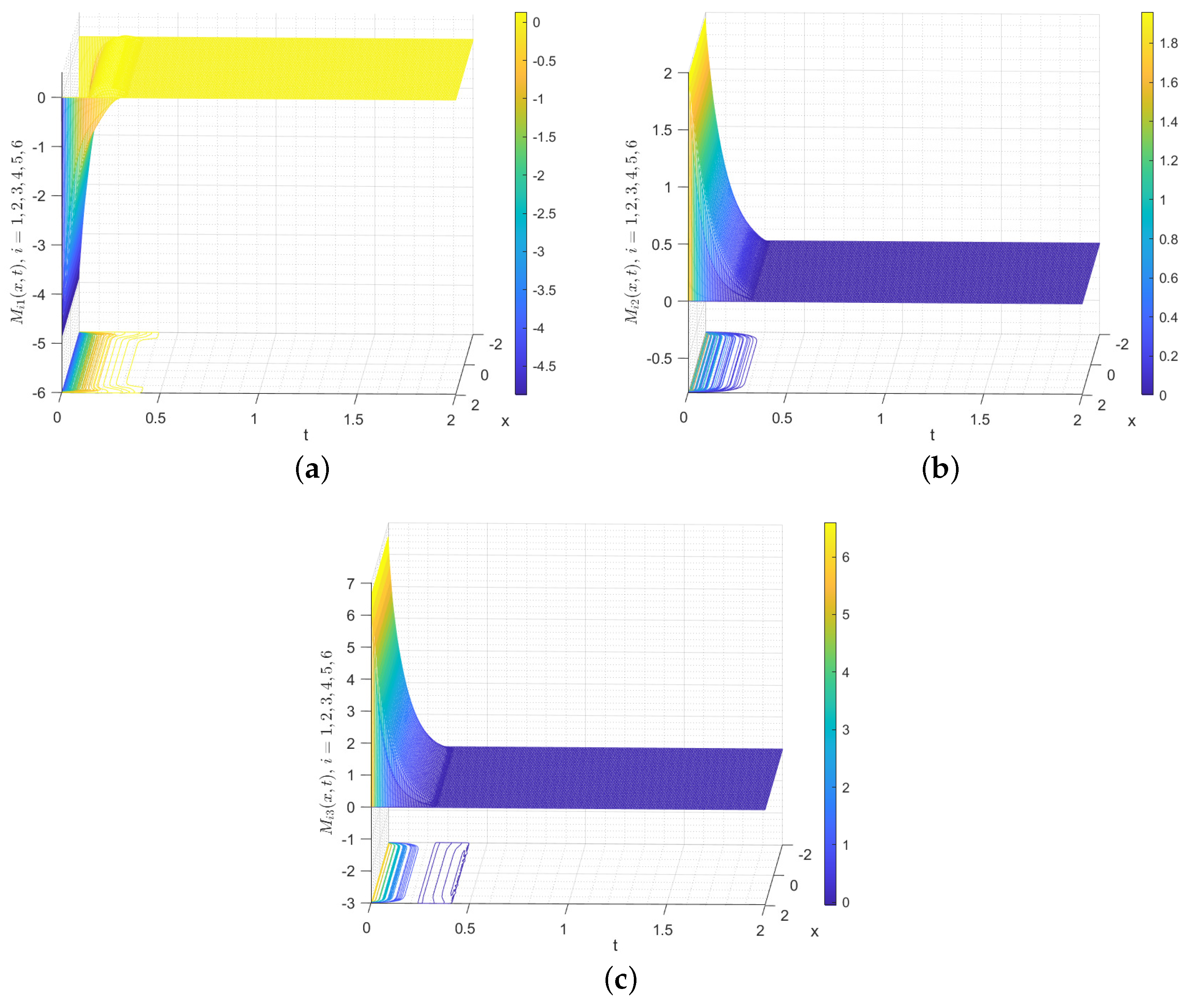
The control parameters of (35) are designed as follows: $\delta =3.897, \sigma =0.2$. The time evolutions of $M_{ij}(x,t)$ under the control law (35) are depicted in Figure 14, which show that $M_{ij}(x,t)$ gradually converges to 0. The estimated upper bound for ST is 1.12.

Figure 15 describes the spatiotemporal evolutions of $M_{ij}(x,t)$ with contour map, which makes it clear that $M_{ij}(x,t)$ gradually converges to 0 during its spatiotemporal evolutione without any alteration in height.

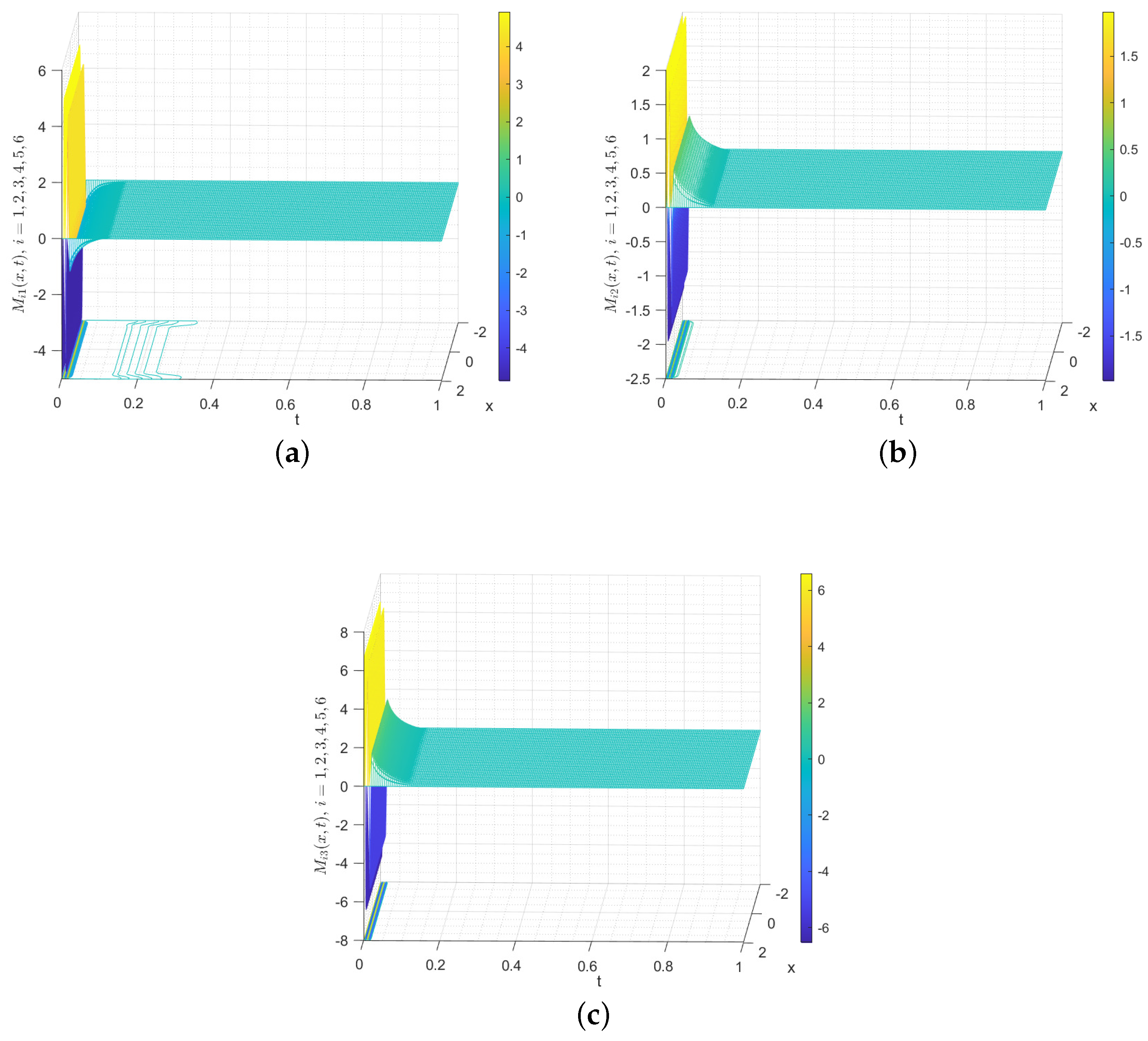
The time evolution of each component of $m_i(x,t)$ and $s(x,t)$ are depicted in Figure 16, which indicate that the states of the network nodes in system (40) and FOSN (41) ultimately achieve BS.

Therefore, FNBS is achieved for system (40) with FOSN (41), which verifies the correctness of the developed control law (35).

Remark 13. 

In contrast to the control protocol (20) in polynomial form and the control protocol (30) which incorporates the linear term as well as the HSF, the control law (35) not only has fewer control parameters and a simpler exhibition without the linear terms, but also effectively reduces the ST (ST (35) < ST (30) < ST (20)) under smaller control gains. The superiority of the control law (35) based on the HSF is attested by its swifter convergence rate, the tighter bound of ST, and the suppression of chattering both in theory and simulations. This is extremely significant in practical applications, especially in engineering problems requiring a high control intensity or rapid control response.

Using the controller designed in [7]: $U_{0i}(x,t)=-\frac{7.49sign\left(M_i(x,t)\right)e^{0.1G^{0.25}\left(t\right)}}{|M_i(x,t)|}$. Figure 17a describes the control inputs of the control law (35) in this work and [7]. Figure 17b depicts the synchronization error of the control law (35) in this work and [7]. As shown in Figure 17a,b, the control law (35) effectively avoids chattering, increases the smoothness of the control input, and reduces the ST, which further validates the theoretical analysis results presented in Remark 8.

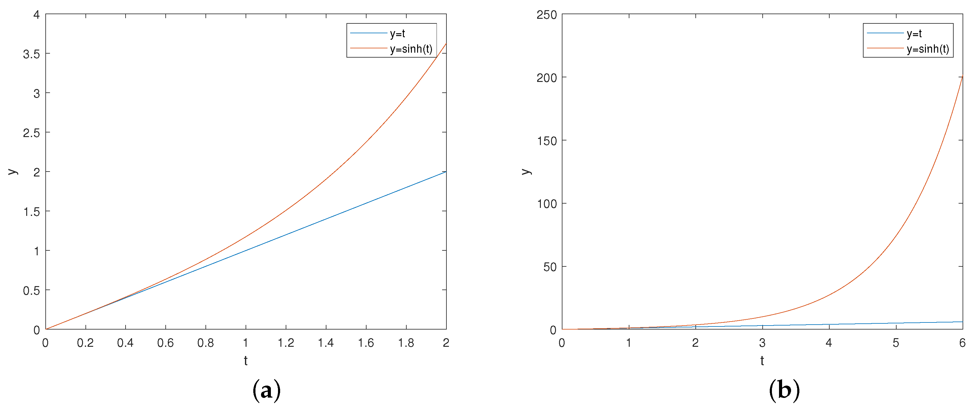
Example 5. 

This example will simulate the HSF to explore why it has excellent qualities in terms of its control performance.

The equivalence measure of the HSF $y=sinh\left(t\right)=\frac{e^t-e^{-t}}{2}$ is $y=\frac{e^t}{2}$, for  $t\to \infty$.  $y=sinh\left(t\right)\le \frac{e^t}{2}$, for  $t\ge 0$. The evolutions of $y=t$ and $y=sinh\left(t\right)$ are depicted in Figure 18. It indicate that the HSF can provide control inputs at an exponential function level, yielding very noticeable control effects. This elucidates why the the error convergence rate is much faster under the control law (35) compared to the control protocols (20) and (30).

Subsequently, we conducted a further analysis for the effectiveness of the control law (35), by applying the methodology of sensitivity analysis. By performing these calculations, one can derive $\left|\frac{\partial U_i(x,t)}{\partial \sigma }\right|=cz(e^z+e^{-z})$, where c is a positive constant and $z=G^{\sigma }$. In other words, the absolute value of the partial derivative of $U_i(x,t)$ with respect to σ equals the product of the exponential function and the power function, which shows that parameter σ significantly influences this control effect. The analysis regarding δ was similar, so it will not be shown again here. These results indicate that the control intensity is very convenient to adjust, which is a desired feature in practical scenarios.

5. Image Encryption and Decryption

Following the theory of limited-time chaotic synchronization, this section demonstrates image encryption and decryption as an application of Theorem 3.

5.1. The Algorithm of Image Encryption and Decryption

A flowchart of image encryption and decryption algorithm is presented in Figure 19. The image encryption algorithm is described in detail below.

Step 1. Preprocess the plaintext image. Import the plaintext image to be encrypted as P. Let $R=P(:,:,1),G=P(:,:,2),$ and $B=P(:,:,3).$$[m,n]=size\left(R\right).$

Step 2. Chaotic system-based secret code streams generator. Following the estimated ST, extract the pseudo-random sequences $s{1}_{1\times mn}$, $s{2}_{1\times 2mn}$ and $s{3}_{1\times mn}$ from the 2-scroll, 3-scroll, and 4-scroll attractors previously discussed. Further disrupt these pseudo-random sequences to obtain the chaotic system-based secret code streams, which can be executed as follows:

$$S1=\odot \left[floor((s1+100)\times {10}^{14})\right]+1,$$

$$S2=\odot \left[floor((s2+100)\times {10}^{14})\right]+1,$$

$$S3=\odot \left[floor((s3+100)\times {10}^{14})\right]+1,$$

where $floor$ refers to the operation used for rounding down and ⊙ signifies the modulo 256 operation.

Step 3. Forward diffusion. To enhance the effectiveness of encryption, we modified each pixel’s value by a forward diffusion algorithm. The specific calculation rules are expressed as Algorithm 2.

Step 4. Arnold’s cat map-based permutation. With forward diffusion, the pixel values undergo distinct changes. Further scrambling operations lead to additional disruption of the pixel locations. Let $a=S2(1:mn)$ and $b=S2(mn+1:2mn)$. Scramble every element $(1,k)$ of $KR$, $KG$, and $KB$ by q, calculated with the following equation:

$$\left[\begin{array}{c}p\\ q\end{array}\right]=\left[\begin{array}{cc}1& a\\ b& ab+1\end{array}\right]\left[\begin{array}{c}1\\ l\end{array}\right].$$

Step 5. Backward diffusion. Since forward diffusion only distributes information from partial pixels across the full image, while a large amount of pixel information is still limited in local areas, we conducted backward diffusion to disseminate each pixel’s information throughout the entire image to enhance the security and resilience of the encryption algorithm. The specific calculation rules are expressed as Algorithm 2. At this point, the plaintext image has been encrypted to generate the ciphertext image.

As the Forward diffusion presented above, as well as the Arnold’s cat map-based permutation and Backward diffusion, are reversible, the decryption process only consists of reversing the steps used in encryption. Notably, the image decryption process is grounded in the time series of FOSN (41) under the control law (35).

Algorithm 2 Bidirectional Diffusion

Input: Plainnext image

Output: Diffused image

START

1:   Set the secret key parameters in this location $KR\left(0\right)=1$; $KG\left(0\right)=1$; $KB\left(0\right)=1$;

Forward Diffusion

2:    $KR\left(1\right)=KR\left(0\right)⨁S1\left(1\right)⨁R\left(1\right)$;

3:    $KG\left(1\right)=KG\left(0\right)⨁S1\left(1\right)⨁G\left(1\right)$;

4:    $KB\left(1\right)=KB\left(0\right)⨁S1\left(1\right)⨁B\left(1\right)$;

5:   for i = 2 to mn do

6:          $KR\left(i\right)=KR(i-1)⨁S1\left(i\right)⨁R\left(i\right)$;

7:          $KG\left(i\right)=KG(i-1)⨁S1\left(i\right)⨁G\left(i\right)$;

8:          $KB\left(i\right)=KB(i-1)⨁S1\left(i\right)⨁B\left(i\right)$;

9:   end for

Backward Diffusion

10:   Set the secret key parameters in this location $KkR\left(0\right)=0$; $KkG\left(0\right)=0$;

$KkB\left(0\right)=0$;

11:    $KkR\left(mn\right)=KkR\left(0\right)⨁S3\left(mn\right)⨁KR\left(mn\right)$;

12:    $KkG\left(mn\right)=KkG\left(0\right)⨁S3\left(mn\right)⨁KG\left(mn\right)$;

13:    $KkB\left(mn\right)=KkB\left(0\right)⨁S3\left(mn\right)⨁KB\left(mn\right)$;

14:   for j = mn − 1 to 1 do

15:          $KkR\left(j\right)=KkR(j+1)⨁S3\left(j\right)⨁KR\left(j\right)$;

16:          $KkG\left(j\right)=KkG(j+1)⨁S3\left(j\right)⨁KG\left(j\right)$;

17:          $KkB\left(j\right)=KkB(j+1)⨁S3\left(j\right)⨁KB\left(j\right)$;

18:   end for

EXIT

The encrypted object in the experiment is the Quick Response (QR) code, as shown in Figure 20a, where the scanned results are “Chaotic Encryption by Finite-time Bipartite Synchronization of Fractional-order Spatiotemporal Networks” and “8364”, as described in Figure 20b. The ciphertext image shows noise-like patterns, without leakage of the visual information in terms of visuals, as described in Figure 20c. No hidden information from the plaintext image can be obtained by scanning the ciphertext image. Figure 20d depicts the decrypted image, which shows consistent results, as described in Figure 20b “Chaotic Encryption by Finite-time Bipartite Synchronization of Fractional-order Spatiotemporal Networks” and “8364”, with the plaintext image. Such impressive results indicate the effectiveness of the designed encryption–decryption algorithm based on the HSF control-based FNBS of FOSN.

5.2. Security Analysis and Tests

To illustrate the validity of the proposed image encryption-decryption system based on the HSF control-based FNBS of FOSN, several classic statistical analysis tests are essential.

5.2.1. Histogram Analyses and ${\chi }^2$ Test

The histogram, a essential metric to reflect the distribution information of every pixel in a grayscale space, reveals the fundamental statistical information of the image. An excellent encryption algorithm is expected to have a uniform distribution of gray levels to minimize the statistical cues available to potential attackers. Figure 21 depicts the histograms of plaintext image and ciphertext image. It is evident from Figure 21 that the histogram of the plaintext image fluctuates significantly, with substantial variations between the peaks and valleys, but the histogram of the ciphertext image tends toward a uniform distribution, eliminating the distribution information of the plaintext image.

To evaluate the quality of the encryption algorithm from the perspective of uniform distribution, the ${\chi }^2$ test is introduced. The ${\chi }^2$ test is conducted to evaluate the consistency of the histogram distribution. Specifically, a lower test value reflects greater consistency in the histogram, which can be calculated with the following equation:

$${\chi }^2={\displaystyle \sum _{i=0}^{255}}\frac{(Car{d}_i-mn/256)}{mn/256},$$

where $Car{d}_i$ refers to the observed frequency of pixels for grey level i. The computed ${\chi }^2$ test values are shown in

Table 1. ${\chi }^2$ test values.

Image	R Channel	G Channel	B Channel
Plain Image	21,374,609.0996	21,374,609.0996	21,374,609.0996
Cipher Image	254.7695	254.7695	254.7695

. The critical value, with a $\alpha =1\%$ significance level and 256 degrees of freedom, is ${\chi }_{0.01}^2=310.4574$. According to Table 1, the ${\chi }^2$ test values for the plaintext image are consistently greater than the theoretical values, whereas the test values for the ciphertext images consistently fall below the standard values. This means that, at the $\alpha =1\%$ significance level, the hypothesis that the histogram follows a consistent distribution cannot be rejected, which indicates that the proposed encrypted–decrypted algorithm successfully safeguards against attacks trying to access the histogram.

5.2.2. Correlation Analysis of Adjacent Pixels in Scatter Diagram and Pearson Correlation Coefficients

In general, there is a substantial correlation among adjacent pixels in plaintext images, which enables attackers to analyze the plaintext image. To safeguard against these statistical attacks, it is imperative to decrease this correlation.

A random selection is made of $n=50,000$ pairs of adjacent pixels $(x_i,y_i)$ in four distinct directions: horizontal, vertical, positive diagonal, and counter diagonal. The distribution of adjacent pixel values in the four distinct directions of the plain and cipher images are presented in Figure 22. It is apparent that there is a strong and positive correlation relationship ofthr plaintext image in the four distinct directions of adjacent pixels, as shown in Figure 22(a1,b1,c1,d1). As outlined in Figure 22(a2,b2,c2,d2), the proposed encryption–decryption algorithm effectively eradicated this correlation to ensure uniformity in the ciphertext image and minimize correlations, thus ensuring that the ciphertext image is statistically unpredictable.

To enable a quantitative analysis of the correlation, the Pearson correlation coefficient ${\rho }_{xy}$ is introduced, which can be calculated as follows:

$${\rho }_{xy}=\frac{cov(X,Y)}{\sqrt{D\left(X\right)}\sqrt{D\left(Y\right)}},$$

where $X=\{x_1,x_2,...,x_n\}$, $Y=\{y_1,y_2,...,y_n\}$; $cov$ denotes the co-correlation coefficient; D represents the variance.

Table 2. The Pearson correlation coefficients.

Image	Plaintext Image			Ciphertext Image
	R	G	B	R	G	B
Horizontal	0.9778	0.9784	0.9785	−0.0005	−0.0004	−0.0001
Vertical	0.9779	0.9783	0.9777	−0.0004	−0.0004	0.0011
Main Diagonal	0.9562	0.9566	0.9567	−0.0039	−0.0060	−0.0023
Counter Diagonal	0.9566	0.9568	0.9563	0.0052	0.0024	0.0042

offers an overview of the adjacent pixels Pearson correlation coefficients in four distinct directions for plaintext image and ciphertext image. One can observe that the correlation coefficients are all close to 1 in the four distinct directions for the plaintext image. However, the correlation coefficients are all close to 0 in the four distinct directions for the ciphertext image. This remarkable performance reveals that the encryption algorithm has strong resistance to statistical attacks, lowering the risks of using the ciphertext.

5.2.3. Information Entropy Test

Ideally, the ciphertext image is expected to contain significant uncertainty and randomness, restricting statistical insights for potential attackers. Therefore, the information entropy test was introduced, where higher values imply fewer differences in grayscale value distribution and a lower risk of information exposure. The calculation formula is shown below:

$$H\left(s\right)=-{\displaystyle \sum _{i=0}^{255}}p\left(s_i\right)lo{g}_{2}p\left(s_i\right),$$

where $p\left(s_i\right)$ denotes the probability of occurrence for the $ith$ signal, indicating that the information entropy of an 8-bit random grayscale image is 8.

Table 3. The information entropy test results.

Image	R Channel	G Channel	B Channel
Plain Image	2.877934	2.877934	2.877934
Cipher Image	7.999299	7.999299	7.999299

presents a general outline of the information entropy values for plaintex and ciphertex images on different colour channels, which shows the superiority of the proposed encryption algorithm owing to its unpredictability and randomness.

5.2.4. Key Sensitivity Analysis

An effective encryption system requires its key parameters to be highly sensitive to thwart attackers trying to crack the ciphertext using brute-force or guessing techniques. We will implement a slight alteration to the key parameters $s^0\left(x\right)+{({10}^{-14},0,0)}^T$. Decrypting Figure 20c using the chaotic sequence derived from the changed initial values, one can obtain the decrypted image, as shown in Figure 23. There is a marked difference between Figure 23 and the plaintext image (Figure 20a), which does not provide the information included in Figure 20b after scanning. Therefore, it can be concluded that the designed encryption–decryption system is sensitive to key variations, granting it significant resistance to differential attacks.

5.2.5. Resistance to Noise Attacks

Encrypted images can be subjected to various disturbances during transmission, resulting in various forms of noise, such as salt–pepper noise, Gaussian noise, and speckle noise. Therefore, it is essential for the encryption–decryption algorithm to decrypt the infected images to evaluate its ability to withstand noise attacks. Therefore, $5\%$ salt–pepper noise, $5\%$ Gaussian noise, and $3\%$ speckle noise were introduced. Adding $5\%$ salt–pepper noise to the image shown in Figure 20c resulted in the image shown in Figure 24(a1), with Figure 24(a2) showing the corresponding decrypted image. Although Figure 20(a2) contains a great deal of noise, it is still possible to yield the information contained in Figure 20b. Adding $5\%$ Gaussian noise to the image shown in Figure 24(a1) resulted in the image shown in Figure 24(b1), with Figure 24(b2) showing the corresponding decrypted image. Although Figure 24(b2) contains more significant noise, it is still possible to yield the information contained in Figure 20b. Adding $3\%$ speckle noise to the image shown in Figure 24(b1) resulted in the image shown in Figure 24(c1), with Figure 24(c2) containing the corresponding decrypted image. Although Figure 24(c2) contains more significant noise, it is still possible to yield the information contained in Figure 20b. This confirms that the proposed encryption–decryption algorithm is able to resist noise attacks to anextent.

5.2.6. Anti Shear Attacks

The ciphertext image may lose some of its information during transmission due to malicious assaults by attackers;.tTerefore, it is indispensable for an encryption–decryption algorithm to decrypt the incomplete image to evaluate its ability to resist shear attacks.

Adding a center shear attack at 25% intensity to the image in Figure 20a resulted in the image shown in Figure 25(a1), with Figure 25(a2) sshowhng the image under bidirectional diffusion and Figure 25(a3) showing the corresponding decrypted image. Although Figure 25(a2) appears to be missing some information, the corresponding decrypted image is still recognizable and can yield the information contained in Figure 20b.

Adding a perimeter shear attack at 50% intensity to the image shown in Figure 20a resulted in the image shown in Figure 25(b1), with Figure 25(b2) showing the image under bidirectional diffusion and Figure 25(b3) showing the corresponding decrypted image. Although Figure 25(b2) appears to be missing more information, the corresponding decrypted image is still recognizable and can be used to yield the information contained in Figure 20b. This demonstrates the efficacy of the bidirectional diffusion algorithm, which enables the encryption and decryption techniques to be robust against specific types of shear attacks.

Remark 14. 

It is highly valuable to compare the performances of the image encryption algorithm we designed and the AES (Advanced Encryption Standard), which is a widely adopted image encryption standard developed by the U.S. National Institute of Standards and Technology. The comparison is depicted in the table below which was carried out by the standard 10-round AES-128 algorithm. As shown in

Table 4. The performances of the AES encryption algorithm.

	Entropy	Pearson Correlation Codfficients				Time
		Horizontal	Vertical	Diagonal	Counter Diagonal
AES	7.9806	−0.0022	0.0469	−0.0259	0.0049	60.2783 s

, the entropy of our designed encryption algorithm is larger than that of the AES, which suggests that the ciphertext generated by our algorithm exhibits more randomness. Furthermore, the correlation between the ciphertext images in our algorithm is lower than that in the AES, indicating greater security in our designed algorithm. According to Figure 19, our encryption algorithm has a simpler structure compared to the AES. From an abstract viewpoint, the Arnold’s cat map, forward diffusion, and backward diffusion used in this paper have the same methods as S-box, ShiftRows, and AddRoundKey in the AES. In addition, the times required for our algorithm and AES are 8.1675 s and 60.2783 s, respectively. Therefore, the encryption algorithm designed in this work demonstrates significant application value.

Remark 15. 

It is important to highlight that the extracted pseudo-random sequence for the chaotic system-based secret code streams generator follows the estimated ST. Actually, the starting time is highly flexible. For example, one can choose $T=(1+\theta )ST$ as the starting time, where parameter θ is related to the plaintext image (if the maximum pixel value of the plaintext image is 0, set $\theta =0$).

$$\theta =\frac{meanpixelvalueoftheplaintextimage+medianpixelvalueoftheplaintextimage}{2\ast maximumpixelvalueoftheplaintextimage}.$$

The plaintext-related parameter T ensures that the equivalent key is also linked to the plaintext image, meaning that the parameter helps protect against key information leakage during the analysis of specific images formed by identical pixel values. Therefore, the encryption algorithm designed with the plaintext-related key parameter θ can effectively resist the chosen-plaintext attacks and the chosen-ciphertext attacks.

Remark 16. 

In this work, an image encryption–decryption algorithm was designed based on the characteristics of the devised FO spatiotemporal chaotic system, which contains different numbers of chaotic attractor scrolls in different positions, employing the derived HSF control law for FNBS of FOSN. In contrast to the ordinary differential equations-based image encryption–decryption algorithms, this paper simultaneously used 2-scroll, 3-scroll, and 4-scroll chaotic attractors to encrypt the plaintext image, which enhances the security and the attack resistance ability. Moreover, the excellent control obtained of the control law (35) significantly reduces the time required for image encryption and decryption, further increasing the risk-resistance of the image encryption–decryption system, showing the effectiveness and superiority of the devised control law based on the HSF.

Remark 17. 

Evidently, the tighter bound on settling time will reduce the time required for image encryption and decryption, which is vital in protecting against malicious hackers. Hence, the tighter bound on settling time increases the risk-resistance of the image encryption–decryption system. Furthermore, the smoother control input improves the stable dynamic behavior of the system, which will produce a similarly positive effect on the encryption algorithm’s security as the tighter bound on settling time. However, the methods that can quantify these qualities to improve the security parameters (e.g., entropy or correlation coefficients) are lacking. This challenge but interesting question will be the topic of our research in the future.

6. Conclusions

The paper explore the HSF control-based FNBS of an FOSN and its application in image encryption. The addressed networks adequately take into account the nature of anisotropic diffusion, i.e., the diffusion matrix can not only be non-diagonal but also non-square. Subsequently, an equation transformation and an inequality estimate for the anisotropic diffusion term were established, which are fundamental for analyzing the diffusion phenomenon in network dynamics. Three control laws were devised and we present a detailed discussion of the HSF control law’s outstanding performance regarding its swifter convergence rate, the tighter bound of the ST and the suppression of chatter. Furthermore, several simulations were carried out to attest to the correctness of our findings by the designed chaotic system with multi-scroll chaotic attractors, which were tested via bifurcation diagram, Poincaré map, and Turing pattern. Later, a formulated image encryption algorithm was evaluated through imperative security tests, revealing the effectiveness and superiority of the obtained results. Given that the use of a sampling-based control could effectively save the communication source, we will concentrate on the sample-based control protocol for SNs in the future.

References

1. Xiong, K.; Yu, J.; Hu, C.; Wen, S.; Jiang, H. Finite-time synchronization of fully complex-valued networks with or without time-varying delays via intermittent control. Neurocomputing 2020, 413, 173–184. [Google Scholar] [CrossRef]
2. Arianos, S.; Bompard, E.; Carbone, A.; Xue, F. Power grid vulnerability: A complex network approach. Chaos Interdiscip. J. Nonlinear Sci. 2009, 19, 013119. [Google Scholar] [CrossRef] [PubMed]
3. Steven, S. Exploring complex networks. Nature 2001, 410, 268–276. [Google Scholar]
4. Yang, T.; Chua, L. Impulsive stabilization for control and synchronization of chaotic systems: Theory and application to secure communication. IEEE Trans. Circuits Syst. I Fundam. Theory Appl. 1997, 44, 976–988. [Google Scholar] [CrossRef]
5. Wei, X.; Wu, X.; Chen, S.; Lu, J.; Chen, G. Cooperative epidemic spreading on a two-layered interconnected network. SIAM J. Appl. Dyn. Syst. 2018, 17, 1503–1520. [Google Scholar] [CrossRef]
6. Sheng, S.; Zhang, X.; Lu, G. Finite-time outer-synchronization for complex networks with Markov jump topology via hybrid control and its application to image encryption. J. Frankl. Inst. 2018, 355, 6493–6519. [Google Scholar] [CrossRef]
7. Liu, Z.; Cai, Y.; Xin, H.; Hu, C.; Shi, T. Exponential control-based fixed/preassigned-time synchronization of output-coupled spatiotemporal networks with directed topology. Commun. Nonlinear Sci. Numer. Simul. 2024, 139, 108267. [Google Scholar] [CrossRef]
8. Hu, C.; He, H.; Jiang, H. Edge-based adaptive distributed method for synchronization of intermittently coupled spatiotemporal networks. IEEE Trans. Autom. Control 2022, 67, 2597–2604. [Google Scholar] [CrossRef]
9. Huang, C.; Zhang, X.; Lam, H.; Tsai, S. Synchronization analysis for nonlinear complex networks with reaction-diffusion terms using fuzzy-model-based approach. IEEE Trans. Fuzzy Syst. 2021, 29, 1350–1362. [Google Scholar] [CrossRef]
10. Liu, K.; Tian, Y. Research and analysis of deep learning image enhancement algorithm based on fractional differential. Chaos Solitons Fractals 2020, 131, 109507. [Google Scholar] [CrossRef]
11. Niedziela, M.; Wlazło, J. Notes on computational aspects of the fractional-order viscoelastic model. J. Eng. Math. 2018, 108, 91–105. [Google Scholar] [CrossRef]
12. Liu, Z.; Chen, S.; Jing, B.; Yang, C.; Ji, J.; Zhao, Z. Fractional variable-order calculus based state of charge estimation of Li-ion battery using dual fractional order Kalman filter. J. Energy Storage 2022, 52, 104685. [Google Scholar] [CrossRef]
13. Wu, K.; Tang, M.; Liu, Z.; Ren, H.; Zhao, L. Pinning synchronization of multiple fractional-order fuzzy complex-valued delayed spatiotemporal neural networks. Chaos Solitons Fractals 2024, 182, 114801. [Google Scholar] [CrossRef]
14. Liu, P.; Kong, M.; Zeng, Z. Projective synchronization analysis of fractional-order neural networks with mixed time delays. IEEE Trans. Cybern. 2022, 52, 6798–6808. [Google Scholar] [CrossRef]
15. Zhang, X.; Tang, L.; Lü, J. Synchronization analysis on two-layer networks of fractional-order systems: Intralayer and interlayer synchronization. IEEE Trans. Circuits Syst. I Regul. Pap. 2020, 67, 2397–2408. [Google Scholar] [CrossRef]
16. Altafini, C. Consensus problems on networks with antagonistic interactions. IEEE Trans. Autom. Control 2013, 58, 935–946. [Google Scholar] [CrossRef]
17. Xu, Y.; Lin, T.; Liu, X.; Li, W. Exponential bipartite synchronization of fractional-order multilayer signed networks via hybrid impulsive control. IEEE Trans. Cybern. 2023, 53, 3926–3938. [Google Scholar] [CrossRef] [PubMed]
18. Ding, D.; Tang, Z.; Park, J.; Ji, Z. Quasi-bipartite synchronization of derivatively coupled complex dynamic networks: Memory-based self-triggered approach. IEEE Trans. Syst. Man Cybern. Syst. 2024, 54, 1611–1621. [Google Scholar] [CrossRef]
19. Chen, X.; Jia, T.; Wang, Z.; Xie, X.; Qiu, J. Practical fixed-time bipartite synchronization of uncertain coupled neural networks subject to deception attacks via dual-channel event-triggered control. IEEE Trans. Cybern. 2024, 54, 3615–3625. [Google Scholar] [CrossRef] [PubMed]
20. Sun, W.; Li, B.; Guo, W.; Wen, S.; Wu, X. Interval bipartite synchronization of multiple neural networks in signed graphs. IEEE Trans. Neural Netw. Learn. Syst. 2023, 34, 10970–10979. [Google Scholar] [CrossRef]
21. Bhat, S.; Bernstein, D. Finite-time stability of continuous autonomous systems. SIAM J. Control Optim. 2000, 38, 751–766. [Google Scholar] [CrossRef]
22. Wei, Y.; Xie, C.; Zhang, X.; Xu, Y. Finite/Fixed-time synchronization for stochastic multilayer networks with pinning control. IEEE Access 2024, 12, 79667–79674. [Google Scholar] [CrossRef]
23. Weng, H.; Yang, Y.; Hao, R.; Liu, F. Finite-Time projective synchronization in fractional-order inertial memristive neural networks: A novel approach to image encryption. Fractal Fract. 2024, 8, 631. [Google Scholar] [CrossRef]
24. Fan, H.; Shi, K.; Guo, Z.; Zhou, A. Finite-time synchronization criteria for caputo fractional-order uncertain memristive neural networks with fuzzy operators and transmission delay under communication feedback. Fractal Fract. 2024, 8, 619. [Google Scholar] [CrossRef]
25. Fan, H.; Chen, X.; Shi, K.; Liang, Y.; Wang, Y.; Wen, H. Mittag-Leffler synchronization in finite time for uncertain fractional-order multi-delayed memristive neural networks with time-varying perturbations via information feedback. Fractal Fract. 2024, 8, 422. [Google Scholar] [CrossRef]
26. Vivekanandhan, G.; Chedjou, J.; Jacques, K.; Rajagopal, K. A unique self-driven 5D hyperjerk circuit with hyperbolic sine function: Hyperchaos with three positive exponents, complex transient behavior and coexisting attractors. Chaos Solitons Fractals 2024, 186, 115276. [Google Scholar] [CrossRef]
27. Volos, C.; Akgul, A.; Pham, V.; Stouboulos, I.; Kyprianidis, I. A simple chaotic circuit with a hyperbolic sine function and its use in a sound encryption scheme. Nonlinear Dyn. 2017, 89, 1047–1061. [Google Scholar] [CrossRef]
28. Deepika, D. Hyperbolic uncertainty estimator based fractional order sliding mode control framework for uncertain fractional order chaos stabilization and synchronization. ISA Trans. 2022, 123, 76–86. [Google Scholar] [CrossRef] [PubMed]
29. Xu, X.; Li, Z.; Yan, T.; Li, E. A novel control approach for the fixed-time synchronization of the complex networks. IEEE Trans. Circuits Syst. II Express Briefs 2022, 69, 2882–2886. [Google Scholar] [CrossRef]
30. Wang, J.; Wu, H.; Huang, T.; Ren, S. Pinning control strategies for synchronization of linearly coupled neural networks with reaction-diffusion terms. IEEE Trans. Neural Netw. Learn. Syst. 2016, 27, 749–761. [Google Scholar] [CrossRef] [PubMed]
31. Hao, R.; Yang, Y.; Liu, F.; Zhou, B. Stability and bipartite synchronization of fractional-order coupled reaction–diffusion neural networks under unbalanced graph. Chaos Solitons Fractals 2024, 189, 115583. [Google Scholar] [CrossRef]
32. Xing, X.; Wu, H.; Cao, J. Event-triggered impulsive control for synchronization in finite time of fractional-order reaction-diffusion complex networks. Neurocomputing 2023, 557, 126703. [Google Scholar] [CrossRef]
33. Qiu, Q.; Su, H. Sampling-based event-triggered exponential synchronization for reaction-diffusion neural networks. IEEE Trans. Neural Netw. Learn. Syst. 2023, 34, 1209–1217. [Google Scholar] [CrossRef]
34. Li, H.; Hu, C.; Zhang, L.; Jiang, H.; Cao, J. Complete and finite-time synchronization of fractional-order fuzzy neural networks via nonlinear feedback control. Fuzzy Sets Syst. 2022, 443, 50–69. [Google Scholar] [CrossRef]
35. Xiong, K.; Hu, C. Fixed-time output synchronization of multilayered coupled networks with quaternion: An exponential quantized scheme. Neurocomputing 2024, 613, 128742. [Google Scholar] [CrossRef]
36. Podlubny, I. Fractional Differential Equations: An Introduction to Fractional Derivatives, Fractional Differential Equations, to Methods of Their Solution and Some of Their Applications; Academic Press: Cambridge, MA, USA, 1998. [Google Scholar]
37. Qin, X.; Jiang, H.; Qiu, J.; Hu, C.; Chen, S.; Ren, Y. Quantized dynamic event-triggered control for fixed/preset-time bipartite synchronization of memristor-based discontinuous multi-layer signed networks. Neurocomputing 2024, 573, 127196. [Google Scholar] [CrossRef]
38. Corwin, L. Multivariable Calculus; Chemical Rubber Company Press: Boca Raton, FL, USA, 2017. [Google Scholar]
39. Yang, S.; Yu, J.; Hu, C.; Jiang, H. Finite-time synchronization of memristive neural networks with fractional-order. IEEE Trans. Syst. Man Cybern. Syst. 2021, 51, 3739–3750. [Google Scholar] [CrossRef]
40. Hu, C.; He, H.; Jiang, H. Fixed/Preassigned-time synchronization of complex networks via improving fixed-time stability. IEEE Trans. Cybern. 2021, 51, 2882–2892. [Google Scholar] [CrossRef]
41. Xu, D.; Song, S.; Su, H. Fixed-time synchronization of large-scale systems via aperiodically intermittent control. Chaos Solitons Fractals 2023, 173, 113613. [Google Scholar] [CrossRef]
42. Ma, X.; Hu, C.; Yu, J.; Wang, L.; Jiang, H. Hyperbolic function-based fixed/preassigned-time stability of nonlinear systems and synchronization of delayed fuzzy Cohen-Grossberg neural networks. Neurocomputing 2024, 567, 127056. [Google Scholar] [CrossRef]
43. Tang, W.; Zhong, G.; Chen, G.; Man, K. Generation of n-scroll attractors via sine function. IEEE Trans. Circuits Syst. I Fundam. Theory Appl. 2001, 48, 1369–1372. [Google Scholar] [CrossRef]
Figure 1. (a) The strange attractor of system (40) at x = 1.33 . (b) The strange attractor of system (40) at x = 0.66 . (c) The strange attractor of system (40) at x = 0 .
Fractalfract 09 00036 g001
Figure 2. (a) The spatiotemporal evolution of s 1 ( x , t ) . (b) The spatiotemporal evolution of s 2 ( x , t ) . (c) The spatiotemporal evolution of s 3 ( x , t ) .
Fractalfract 09 00036 g002
Figure 3. (a) The Turing pattern of s 1 ( x , t ) . (b) The Turing pattern of s 2 ( x , t ) . (c) The Turing pattern of s 3 ( x , t ) .
Fractalfract 09 00036 g003
Figure 4. (a) Bifurcation diagram. (b) Poincaré map: the projection on the plane is 5 x 6.1 y + 0.92 z = 0 .
Fractalfract 09 00036 g004
Figure 5. (a) Network topology. (b) The time evolutions of error M i j ( x , t ) without control.
Fractalfract 09 00036 g005
Figure 6. (a) The spatiotemporal evolutions of M i 1 ( x , t ) with contour map. (b) The spatiotemporal evolutions of M i 2 ( x , t ) with contour map. (c) The spatiotemporal evolutions of M i 3 ( x , t ) with contour map.
Fractalfract 09 00036 g006
Figure 7. (a) The time evolutions of m i 1 ( x , t ) . (b) The time evolutions of m i 2 ( x , t ) . (c) The time evolutions of m i 3 ( x , t ) .
Fractalfract 09 00036 g007
Figure 8. The time evolutions of M i j ( x , t ) under the control protocol (20).
Fractalfract 09 00036 g008
Figure 9. (a) The spatiotemporal evolutions of M i 1 ( x , t ) with contour map under control protocol (20). (b) The spatiotemporal evolutions of M i 2 ( x , t ) with contour map undercontrol protocol (20). (c) The spatiotemporal evolutions of M i 3 ( x , t ) with contour map undercontrol protocol (20).
Fractalfract 09 00036 g009
Figure 10. (a) The time evolutions of s 1 ( x , t ) and m i 1 ( x , t ) . (b) The time evolutions of s 2 ( x , t ) and m i 2 ( x , t ) . (c) The time evolutions of s 3 ( x , t ) and m i 3 ( x , t ) .
Fractalfract 09 00036 g010
Figure 11. The time evolutions of M i j ( x , t ) under the control protocol (30).
Fractalfract 09 00036 g011
Figure 12. (a) The spatiotemporal evolutions of M i 1 ( x , t ) with contour map under control protocol (30). (b) The spatiotemporal evolutions of M i 2 ( x , t ) with contour map under control protocol (30). (c) The spatiotemporal evolutions of M i 3 ( x , t ) , with contour map under control protocol (30).
Fractalfract 09 00036 g012
Figure 13. (a) The time evolutions of s 1 ( x , t ) and m i 1 ( x , t ) . (b) The time evolutions of s 2 ( x , t ) and m i 2 ( x , t ) . (c) The time evolutions of s 3 ( x , t ) and m i 3 ( x , t ) .
Fractalfract 09 00036 g013
Figure 14. The time evolutions of M i j ( x , t ) under the control law (35).
Fractalfract 09 00036 g014
Figure 15. (a) The spatiotemporal evolutions of M i 1 ( x , t ) with contour map under control law (35). (b) The spatiotemporal evolutions of M i 2 ( x , t ) with contour map under control law (35). (c) The spatiotemporal evolutions of M i 3 ( x , t ) with contour map under control law (35).
Fractalfract 09 00036 g015
Figure 16. (a) The time evolutions of s 1 ( x , t ) and m i 1 ( x , t ) . (b) The time evolutions of s 2 ( x , t ) and m i 2 ( x , t ) . (c) The time evolutions of s 3 ( x , t ) and m i 3 ( x , t ) .
Fractalfract 09 00036 g016
Figure 17. (a) The control inputs of the control law (35) in this work and [7]. (b) The synchronization errors in this work and [7]. ( U 0 i ( x , t ) and M 0 i ( x , t ) are the controllor and error in [7], respectively).
Fractalfract 09 00036 g017
Figure 18. (a) t [ 0 , 2 ] , y = t and y = s i n h ( t ) . (b) t [ 0 , 6 ] , y = t and y = s i n h ( t ) .
Fractalfract 09 00036 g018
Figure 19. The image encryption and decryption algorithm.
Fractalfract 09 00036 g019
Figure 20. (a) The plaintext image to be encrypted. (b) The content obtained via scanning the plaintext image. (c) The ciphertext image. (d) The decryption image.
Fractalfract 09 00036 g020
Figure 21. (a) The histogram of the plaintext image. (b) The histogram of the ciphertext image.
Fractalfract 09 00036 g021
Figure 22. (a1,b1,c1,d1): The scatter plots of adjacent horizontal, vertical, positive diagonal and counter-diagonal for plaintext image, respectively. (a2,b2,c2,d2): the scatter plots of adjacent horizontal, vertical, positive diagonal and counter diagonal for ciphertext image, respectively.
Fractalfract 09 00036 g022aFractalfract 09 00036 g022b
Figure 23. The decrypted image with s 0 ( x ) + ( 10 14 , 0 , 0 ) T .
Fractalfract 09 00036 g023
Figure 24. (a1) The ciphertext image with 5 % salt–pepper noise. (a2). The decryption image for the ciphertext image with 5 % salt–pepper noise. (b1) The ciphertext image with 5 % salt–pepper noise and 5 % Gaussian noise. (b2) The decryption image for the ciphertext image with 5 % salt–pepper noise and 5 % Gaussian noise. (c1) The ciphertext image with 5 % salt–pepper noise, 5 % Gaussian noise, and 3 % speckle noise. (c2) The decryption image for the ciphertext image with 5 % salt–pepper noise, 5 % Gaussian noise, and 3 % speckle noise.
Fractalfract 09 00036 g024
Figure 25. (a1) The ciphertext image with a center shear attack at 25% intensity. (a2) The diffused ciphertext image with a center shear attack at 25% intensity. (a3) The decryption image for the ciphertext image with a center shear attack at 25% intensity. (b1) The ciphertext image with a perimeter shear attack at 50% intensity. (b2) The diffused ciphertext image with a perimeter shear attack at 50% intensity. (b3) The decryption image for the ciphertext image with a perimeter shear attack at 50% intensity.
Fractalfract 09 00036 g025