Article

Analysis of Infection and Diffusion Coefficient in an SIR Model by Using Generalized Fractional Derivative

by
Ibtehal Alazman
1,
Manvendra Narayan Mishra
2,*,
Badr Saad Alkahtani
3 and
Ravi Shanker Dubey
4
1
Department of Mathematics and Statistics, College of Science, Imam Mohammad Ibn Saud Islamic University (IMSIU), Riyadh 13318, Saudi Arabia
2
Department of Mathematics, Suresh Gyan Vihar University, Jaipur 302017, India
3
Department of Mathematics, College of Science, King Saud University, P.O. Box 1142, Riyadh 11989, Saudi Arabia
4
Department of Mathematics, Amity School of Applied Science, Amity University Rajasthan, Jaipur 303002, India
*
Author to whom correspondence should be addressed.
Fractal Fract. 2024, 8(9), 537; https://doi.org/10.3390/fractalfract8090537
Submission received: 22 August 2024 / Revised: 7 September 2024 / Accepted: 13 September 2024 / Published: 15 September 2024
(This article belongs to the Special Issue Advances in Fractional Modeling and Computation)

Abstract

:
In this article, a diffusion component in an SIR model is introduced, and its impact is analyzed using fractional calculus. We have included the diffusion component in the SIR model. in order to illustrate the variations. Here, we have applied the general fractional derivative to analyze the impact. The Laplace decomposition technique is employed to obtain the numerical outcomes of the model. In order to observe the effect of the diffusion component in the SIR model, graphical solutions are also displayed.

1. Introduction

The application of mathematical models to analyze biological systems has captured significant attention in recent decades. Gregor Mendel pioneered this approach by using mathematics to formulate the laws of heredity, and epidemic modeling dates back to the 19th century. Notably, Ronald Ross revolutionized epidemiology by introducing compartmental models such as SIR and SIRS. In [1], Asif et al. offered a comparative study of the SIR model, while the SEIR model was explored in [2] using advanced modeling techniques. Nisar et al. examined the dynamics of whooping cough through the SIR model in [3], and Ergen et al. made predictions regarding disease progression in [4]. Alqarni et al. provided a focused analysis of whooping cough infection in [5]. Today, mathematical modeling is indispensable across nearly every facet of life, valued for its precision and capacity to address complex real-world constraints [6,7].
In recent years, mathematical modeling is becoming more relevant when it comes together with fractional calculus [8,9,10,11]. Fractional calculus is one of the most important and impactful areas in mathematics due to various useful operators and some very logical concepts. Fractional calculus gives more precise results due to the memory effect of their kernels [12,13,14,15,16].
In current time, fractional calculus is receiving much more attention from many mathematicians and researchers than the integer order system due to the fact that, in fractional calculus, we have much more freedom to be more accurate than the integer order system, as, in fractional calculus, we can have infinite points at which we can analyze the results, while we have limitations in obtaining the results only at integers in the integer ordered system [17,18,19,20,21,22]. There has been remarkable work carried out in various fields of our real life like biological fields, epidemiology, engineering, physical problems, medical science, inventory, mechanical problems and many more [23,24,25,26,27,28].
Now focusing back on our topic, in this paper, we have decided to analyze the effect of diffusion on the system. To be more specific, we have taken the system of an SIR model [4,29,30,31,32] of pertussis. This is a very highly contagious bacterial infection. This infection spreads from person to person through social contact. Pertussis has shown extreme growth in the last few decades. As per a report, around 600,000 deaths per year are caused by pertussis around the globe. The main reason of its spread is airborne discharge from the mucous of infected persons. Vaccination has shown some resistance but is not as effective as it should be. Here, we have taken the SIR model given by G. G. Parra et al. [6]. We have added a diffusion factor into the existing model to analyze its effect. We have used the general fractional derivative along with Laplace transformation to achieve our objective. We have used this particular operator (generalized operator) since we can obtain three different results by just changing the kernel of the function, and we can obtain a comparative analytic view by using three different kernels. We have used the generalized operator here because we can compare the results for a classical operator (RL) with non-singular and non-local operators. One more important thing with this paper is the mentioned SIR model is not described by any of the fractional operators till date, so this is a unique problem which we have tried to discuss and analyze. In this paper, we have used the Riemann Liouville derivative (a kind of generalized derivative) rather than Caputo, since our main objective is to analyze the SIR model by generalized fractional derivatives and not only Caputo. We have also presented the existence and uniqueness of our novel approach, and this approach is well supported by the graphical results of the model as well [33,34,35].
The widespread use of SIR models with fractional derivatives and diffusion coefficients is limited by their complexity, computational costs and difficulty in interpreting parameters, despite the fact that they provide a more sophisticated way to model the spread of disease, especially when memory effects and spatial diffusion are significant.
There are many real world applications of the SIR model which can benefit society. Some examples are as follows: By taking fractional derivatives into account, a fractional SIR model takes the memory component into account and permits the illness to spread based on the system’s past as well as its present condition. It is possible to predict disease patterns more precisely in places like urban centers or refugee camps, where they may differ from those in rural regions. The fractional model accounts for differences in the relative contributions of various areas to the transmission of illness. Vaccines frequently produce waning immunity, which is immunity that takes longer to develop or fades over time. This progressive process can be better simulated by a fractional SIR model than by a normal SIR model. The long-term impacts of vaccination efforts can be better understood thanks to the fractional method.
This article is divided into seven parts. Part one consists of the introduction of the article. Section 2 deals with pre-requisites related to the paper. The SIR model [36,37,38,39] is briefly discussed in Section 3, while Section 4 presents the existence and uniqueness of the solution. In the next segment, we have found the solution of the SIR model by a general fractional derivative with the help of Laplace transform. Graphical results have been presented in Section 6, while the paper is concluded in Section 7. A list of references is attached at the end to acknowledge the researchers and mathematicians.

2. Pre-Requisites

An overview of the recently defined general fractional operator is given in this section. According to [40], scholars have presented the Caputo ([41]) and Riemann–Liouville (RL) derivatives of the fractional exponent, which are shown by
D t γ 0 C f ( t ) = 0 t f ˙ ( s ) ι ( t s ) d s ,
D t γ 0 f ( t ) = d d t 0 t f ( s ) ι ( t s ) d s ,
where γ ( 0 , 1 ) is power of derivative, f : [ 0 , + ) R is a continuous function with f ˙ L loc 1 ( 0 , + ) , 0 t T < + , ι is known as kernel. The linear condition is enforced on the operator,
D t γ 0 C ( j f ( t ) + k g ( t ) ) = j D t γ 0 C f ( t ) + k D t γ 0 C g ( t ) ,
D t γ 0 ( j f ( t ) + k g ( t ) ) = j 0 D t γ f ( t ) + k 0 D t γ g ( t ) .
It is obvious that for any t > 0 , ι ( t ) is met, and a completely function of monotone type ι ( t ) occurs [11],
ι ( t ) ι ( t ) = 0 ι ( s ) ι ( t s ) d s = 1 ,
and further, for f L loc 1 ( 0 , + ) , we can rewrite above like
D t γ 0 D t γ 0 C f ( t ) = f ( t ) f ( 0 ) ,
where D t γ 0 represents the Riemann–Liouville integral of fractional order ([42]), given as
D t γ 0 f ( t ) = 0 t f ( s ) ι ( t s ) d s .
The right Caputo and Riemann–Liouville fractional derivatives are
D T γ t C f ( t ) = t T f ˙ ( s ) r ( s t ) d s ,
D T γ t f ( t ) = d d t t T f ( s ) r ( s t ) d s
and
D T γ t f ( t ) = t T f ( s ) r ( s t ) d s .
The integration by the component formula is thus satisfied by the aforementioned fractional order operators, according to the results in [43].
0 T f ( s ) 0 D s γ g ( s ) d s = 0 T g ( s ) s C D s γ f ( s ) d s ,
0 T f ( s ) 0 D s γ C g ( s ) d s = 0 T g ( s ) s D s γ f ( s ) d s .
By changing various kernels into general operator definitions, we can derive three specific cases of the general operator. In the first case when the kernel is ι ( t ) = t γ Γ ( 1 γ ) , we have the power function ι ( t ) = t γ 1 Γ ( γ ) which reforms the integral operator’s associated kernel (7).
Further, take kernel ι ( t ) = B ( γ ) 1 γ E γ γ 1 γ t γ where E γ and B ( γ ) are Mittag–Leffler and normalization functions. Also, we have
ι ( t ) = 1 γ B ( γ ) δ ( t ) + γ B ( γ ) Γ ( γ ) t γ 1 .
So, Equations (1) and (2) may be used to obtain the derivatives of Atangana–Baleanu–Caputo (ABC) and Atangana–Baleanu–Riemann–Liouville. The AB type integral is [33]
D t γ 0 f ( t ) = 1 γ B ( γ ) f ( t ) + γ B ( γ ) Γ ( γ ) 0 t ( t s ) γ 1 f ( s ) d s .
Now, in the last situation, the Caputo–Fabrizio (CF) derivative ([11]) is found by taking kernel ι ( t ) = B ( γ ) 1 γ exp γ 1 γ t .

2.1. Riemann–Liouville’s Fractional Operator

Riemann–Liouville’s fractional operator ([44]) is explained below:
D x α R L f ( x ) = 1 Γ n α d n d x n 0 x x y n α 1 f ( y ) d y ,
where α is the order of the derivative, and 0 < α < 1 .

2.2. Caputo–Fabrizio Fractional Derivative

Let h H 1 ( a 1 , b 1 ) , b 1 > a 1 , β [ 0 , 1 ] ; then, the new Caputo–Fabrizio derivative of fractional order ([45]) is as follows:
D t β h ( t ) = M ( β ) 1 β a t h x e β t x 1 β dx .
M ( α ) is a function of normalization such that M ( 0 ) = M ( 1 ) = 1 . If the function does not belong to H 1 ( a 1 , b 1 ) , then, the derivative is
D t β h ( t ) = N ( ρ ) ρ a t h x e t x ρ dx , N ( 0 ) = N ( ) = 1 ,
and more than that,
lim ρ 0 1 ρ e t x 1 β = δ ( x t ) .

2.3. Atangana–Baleanu Fractional Derivative

Let h H ( 0 , 1 ) ; then, the Atangana–Baleanu fractional derivative (in Caputo) ([17]) of order α is
T α ( h ) ( x ) = B ( α ) 1 α 0 x E α α 1 α ( x s ) α h ( s ) d s ,
where B ( α ) > 0 is a normalizing function which agrees to B(0) = B(1) = 1, and E α is the Mittag–Leffler function.

2.4. Laplace Transform

The Laplace transformation ([46]) is an important transform in mathematics. It usually converts the system to an algebraic system, which is easily solvable. The Laplace transform of f ( t ) is represented by L { f ( t ) } and is explained as
L { f ( t ) } = 0 e s t f ( t ) d t , s > 0 .

2.4.1. Laplace Transform of Riemann–Liouville Fractional Differential Operator

The Laplace transform of Riemann–Liouville’s fractional derivative is explained below:
L D γ C g ( t ) = [ s L ( g ( t ) ) g ( 0 ) ] s ( γ 1 ) .

2.4.2. Laplace Transform of Caputo–Fabrizio Fractional Differential Operator

The Laplace transformation of CF operator is as follows:
L D γ C F g ( t ) = 1 2 . B ( γ ) ( 2 γ ) 1 γ . s L { g ( t ) } g ( 0 ) s + γ 1 γ .

2.4.3. Laplace Transform of Atangana–Baleanu Fractional Differential Operator

Let D α A B C f ( t ) be the Atangana–Baleanu fractional differential operator of any function f ( t ) ; then, the Laplace transform of the Atangana–Baleanu fractional differential operator is defined as follows:
L { D α A B C f ( t ) } = M ( α ) 1 α p α L { f ( t ) } p α 1 f ( 0 ) p α + α 1 α .

3. SIR Model

We have considered an SIR model ([1,47,48]) having three compartments or sub classes for the given population, namely, susceptible class S ( t ) , infected class I ( t ) and recovered class R ( t ) . The total population is represented by N and is defined as N = S + I + R .
In this system, to study the effect of diffusion, we added the diffusion term in each equation of the system; hence, the system reduces to
d S d t = μ μ S N γ S I + α 2 S x 2 d I d t = N γ S I μ I ν I + α 2 I x 2 d R d t = ν I μ R + α 2 R x 2 ,
with the condition that S + I + R = 1 . In this system, μ is the birth rate, γ is the transmission rate, ν is the recovery rate, and N is the total population and is supposed to be constant. Here, α is the diffusion constant of susceptible, infected and recovered classes, respectively. One important thing to be noted is that we have taken the interval [0, 0.25] as the domain for the given SIR model. Here, the initial conditions for S ( t ) , I ( t ) and R ( t ) are given as follows:
S 0 = c 1 exp 10 x 2 , 0 x 0.25 , I 0 = c 2 exp 100 x 2 , 0 x 0.25 , R 0 = c 3 , 0 x 0.25 .
In coming sections, we will use model (25) and set of conditions (25) to achieve our objective.

4. Existence and Uniqueness of Result

Here, we will establish the existence of the result of the model for all three different kernels of the generalized derivative.

4.1. In Caputo–Fabrizio Derivative Case

4.1.1. Theorem 1

Define N 1 , N 2 , N 3 and their connection to the variables.
Proof. 
The given system is as follows:
D t β 0 C F S ( t ) = μ μ S N γ S I ,
D t β 0 C F I ( t ) = N γ S I μ I ν I ,
D t β 0 C F R ( t ) = ν I μ R .
Here, 0 < β 1 . Then, converting the above model into integral equations,
S ( t ) S ( 0 ) = I t β 0 C F [ μ μ S N γ S I ] ,
I ( t ) I ( 0 ) = I t β 0 C F [ N γ S I μ I ν I ] ,
R ( t ) R ( 0 ) = I t β 0 C F [ ν I μ R ] .
Then, by Nieto’s definition, we obtain
S ( t ) = S ( 0 ) + 2 ( 1 β ) ( 2 β ) B ( β ) [ μ μ S N γ S I ] + 2 β ( 2 β ) B ( β ) 0 t μ μ S N γ S I d s ,
I ( t ) = I ( 0 ) + 2 ( 1 β ) ( 2 β ) B ( β ) N γ S I μ I ν I + 2 β ( 2 β ) B ( β ) 0 t N γ S I μ I ν I d s ,
and
R ( t ) = R ( 0 ) + 2 ( 1 β ) ( 2 β ) B ( β ) [ ν I μ R ] + 2 β ( 2 β ) B ( β ) 0 t ν I μ R d s .
Furthermore, consider the kernels are
N 1 ( t , S ) = μ μ S N γ S I ,
N 2 ( t , I ) = N γ S I μ I ν I ,
N 3 ( t , R ) = ν I μ R .

4.1.2. Theorem 2

Show that N 1 , N 2 and N 3 satisfy the Lipschitz condition.
Proof. 
We shall prove for N 1 at first. Assume S and S 1 are two functions; hence,
N 1 ( t , S ) N 1 ( t , S 1 ) μ μ S N γ S I μ μ S 1 N γ S 1 I , = μ S 1 S + N γ I S 1 S , = μ + N γ I S 1 S ,
N 1 ( t , S ) N 1 ( t , S 1 ) H S 1 ( t ) S ( t ) , w h e r e μ + N γ I H < 1 .
Similarly,
N 2 ( t , I ) N 2 ( t , I 1 ) N γ S I μ I ν I N γ S I 1 μ I 1 ν I 1 , ( μ + ν N γ S ) I 1 ( t ) I ( t ) .
N 2 ( t , I ) N 2 ( t , I 1 ) H 1 I 1 ( t ) I ( t ) , w h e r e ( μ + ν N γ S ) H 1 < 1 .
and
N 3 ( t , R ) N 3 ( t , R 1 ) ν I μ R ν I μ R 1 , μ R 1 ( t ) R ( t ) .
N 3 ( t , R ) N 3 ( t , R 1 ) H 2 R 1 ( t ) R ( t ) , w h e r e μ H 2 < 1 .
Now, by recursive relation,
S n ( t ) = 2 ( 1 β ) ( 2 β ) B ( β ) N 1 ( t , S n 1 ) + 2 β ( 2 β ) B ( β ) 0 t N 1 ( s , S n 1 ) d s ,
I n ( t ) = 2 ( 1 β ) ( 2 β ) B ( β ) N 2 ( t , I n 1 ) + 2 β ( 2 β ) B ( β ) 0 t N 2 ( s , I n 1 ) d s ,
and
R n ( t ) = 2 ( 1 β ) ( 2 β ) B ( β ) N 3 ( t , R n 1 ) + 2 β ( 2 β ) B ( β ) 0 t N 3 ( s , R n 1 ) d s .
Now, consider the difference between two successive terms is
U n ( t ) = S n ( t ) S n 1 ( t ) = 2 ( 1 β ) ( 2 β ) B ( β ) N 1 ( t , S n 1 ) + 2 β ( 2 β ) B ( β ) 0 t N 1 ( s , S n 1 ) d s 2 ( 1 β ) ( 2 β ) B ( β ) N 1 ( t , S n 2 ) 2 β ( 2 β ) B ( β ) 0 t N 1 ( s , S n 2 ) d s ,
U n ( t ) = 2 ( 1 β ) ( 2 β ) B ( β ) N 1 ( t , S n 1 ) 2 ( 1 β ) ( 2 β ) B ( β ) N 1 ( t , S n 2 ) + 2 β ( 2 β ) B ( β ) 0 t N 1 ( s , S n 1 ) N 1 ( s , S n 2 ) d s .
Now,
U n ( t ) = S n ( t ) S n 1 ( t ) = 2 ( 1 β ) ( 2 β ) B ( β ) N 1 ( t , S n 1 ) 2 ( 1 β ) ( 2 β ) B ( β ) N 1 ( t , S n 2 ) + 2 β ( 2 β ) B ( β ) 0 t N 1 ( s , S n 1 ) N 1 ( s , S n 2 ) d s , 2 ( 1 β ) ( 2 β ) B ( β ) N 1 ( t , S n 1 ) N 1 ( t , S n 2 ) + 2 β ( 2 β ) B ( β ) 0 t N 1 ( s , S n 1 ) N 1 ( s , S n 2 ) d s ,
But N 1 satisfies the Lipschitz condition so
U n ( t ) 2 ( 1 β ) ( 2 β ) B ( β ) H S n 1 S n 2 + 2 β ( 2 β ) B ( β ) J 0 t S n 1 S n 2 d s .
Similarly, we can obtain
W n ( t ) 2 ( 1 β ) ( 2 β ) B ( β ) H 1 I n 1 I n 2 + 2 β ( 2 β ) B ( β ) J 1 0 t I n 1 I n 2 d s ,
and
Q n ( t ) 2 ( 1 β ) ( 2 β ) B ( β ) H 2 R n 1 R n 2 + 2 β ( 2 β ) B ( β ) J 2 0 t R n 1 R n 2 d s .

4.1.3. Theorem 3

Show that the SIR system with fractional order is the minimal model of dynamics.
Proof. 
By the recursive technique, we obtain
U n ( t ) S ( 0 ) + 2 ( 1 β ) H ( 2 β ) B ( β ) n + 2 β J t ( 2 β ) B ( β ) n ,
W n ( t ) I ( 0 ) + 2 ( 1 β ) H 1 ( 2 β ) B ( β ) n + 2 β J 1 t ( 2 β ) B ( β ) n ,
and
Q n ( t ) R ( 0 ) + 2 ( 1 β ) H 2 ( 2 β ) B ( β ) n + 2 β J 2 t ( 2 β ) B ( β ) n .
Hence, the results are validated and found to be continuous as well. So,
S ( t ) = S n ( t ) + A n ( t ) , I ( t ) = I n ( t ) + C n ( t ) , R ( t ) = R n ( t ) + L n ( t ) ,
where A n , C n and L n are remainders of series solution. So,
S ( t ) S n ( t ) = 2 ( 1 β ) ( 2 β ) B ( β ) N 1 ( t , S n ) + 2 β ( 2 β ) B ( β ) 0 t N 1 ( s , S n ) d s , S ( t ) S n ( t ) = 2 ( 1 β ) ( 2 β ) B ( β ) N 1 ( t , S A n ( t ) ) + 2 β ( 2 β ) B ( β ) 0 t N 1 ( s , S A n ( s ) ) d s .
Similarly, we have
I ( t ) I n ( t ) = 2 ( 1 β ) ( 2 β ) B ( β ) N 2 ( t , I C n ( t ) ) + 2 β ( 2 β ) B ( β ) 0 t N 2 ( s , I C n ( s ) ) d s , a n d R ( t ) R n ( t ) = 2 ( 1 β ) ( 2 β ) B ( β ) N 3 ( t , R L n ( t ) ) + 2 β ( 2 β ) B ( β ) 0 t N 3 ( s , R L n ( s ) ) d s .
Now, it is clear that,
S ( t ) S n ( t ) = 2 ( 1 β ) ( 2 β ) B ( β ) N 1 ( t , S A n ( t ) ) + 2 β ( 2 β ) B ( β ) 0 t N 1 ( s , S A n ( s ) ) d s ,
S ( t ) S ( 0 ) 2 ( 1 β ) N 1 ( t , S ) ( 2 β ) B ( β ) 2 β ( 2 β ) B ( β ) 0 t N 1 ( s , S ) d s = A n ( t ) + 2 ( 1 β ) N 1 ( t , S A n ( t ) ) ( 2 β ) B ( β ) + 2 β ( 2 β ) B ( β ) 0 t N 1 ( s , S A n ( s ) ) d s .
Now,
S ( t ) 2 ( 1 β ) N 1 ( t , S ) ( 2 β ) B ( β ) S ( 0 ) 2 β ( 2 β ) B ( β ) 0 t N 1 ( s , S ) d s A n ( t ) + 2 ( 1 β ) H ( 2 β ) B ( β ) + 2 β ( 2 β ) B ( β ) J t A n ( t ) ,
I ( t ) 2 ( 1 β ) N 2 ( t , I ) ( 2 β ) B ( β ) I ( 0 ) 2 β ( 2 β ) B ( β ) 0 t N 2 ( s , I ) d s C n ( t ) + 2 ( 1 β ) H 1 ( 2 β ) B ( β ) + 2 β ( 2 β ) B ( β ) J 1 t C n ( t ) ,
and
R ( t ) 2 ( 1 β ) N 3 ( t , R ) ( 2 β ) B ( β ) R ( 0 ) 2 β ( 2 β ) B ( β ) 0 t N 3 ( s , R ) d s L n ( t ) + 2 ( 1 β ) H 2 ( 2 β ) B ( β ) + 2 β ( 2 β ) B ( β ) J 2 t L n ( t ) .
Now, making n , we obtain
S ( t ) = S ( 0 ) + 2 ( 1 β ) N 1 ( t , S ) ( 2 β ) B ( β ) + 2 β ( 2 β ) B ( β ) 0 t N 1 ( s , S ) d s ,
I ( t ) = I ( 0 ) + 2 ( 1 β ) N 3 ( t , I ) ( 2 β ) B ( β ) + 2 β ( 2 β ) B ( β ) 0 t N 2 ( s , I ) d s ,
and
R ( t ) = R ( 0 ) + 2 ( 1 β ) N 5 ( t , R ) ( 2 β ) B ( β ) + 2 β ( 2 β ) B ( β ) 0 t N 3 ( s , R ) d s .
Based on the aforementioned equations, we can state that the system’s solution exists.
Similarly, when we modify the kernel, we can also demonstrate that the remaining two cases have a solution.

4.2. Uniqueness of Result

Here, we are going to prove that the results mentioned in the above section are totally solitary. For this, we suppose that there exists another set of results for the set up given by Equations (26)–(28), say, S t , I t and R t . Then, we have
S t S 1 t = 2 1 β B β 2 β N 1 ( t , S ) N 1 ( t , S 1 ) + 2 β B β 2 β 0 t N 1 ( s , S ) N 1 ( s , S 1 ) ds ,
and on taking norm both sides, we obtain
S S 1 = 2 1 β B β 2 β N 1 ( t , S ) N 1 ( t , S 1 ) + 2 β B β 2 β 0 t N 1 ( s , S ) N 1 ( s , S 1 ) ds ,
using Lipchitz condition, we obtain
S S 1 < 2 1 β B β 2 β H Z + 2 β B β 2 β J 1 Z t n ,
which is true for all n. So,
S = S 1 ,
Similarly, I = I 1 , and R = R 1 . So, the uniqueness of the solution is proven.
In the same way, we can also show the uniqueness of the solution for the other two cases.

5. Solution of SIR Model Based on General Fractional Derivative by Using Laplace Transform

Here, to study the effect of diffusion, we add the diffusion term in each equation of the system:
d S d t = μ μ S N γ S I + α 2 S x 2 d I d t = N γ S I μ I ν I + α 2 I x 2 d R d t = ν I μ R + α 2 R x 2 .
But we are interested in the solution by using the general operator of fractional order. So, we develop another system with the general fractional operator of order β . Hence,
D β c S ( t ) = μ μ S N γ S I + α 2 S x 2 D β c I ( t ) = N γ S I μ I ν I + α 2 I x 2 D β c R ( t ) = ν I μ R + α 2 R x 2 ,
where D β c represents the general operator of fractional order β . Now, applying Laplace transform on both sides in the first equation of system (40), we obtain
L D β c S ( t ) = L μ μ S N γ S I + α 2 S x 2 .
By incorporating the various kernels into the various general operator definitions, we may derive three specific cases of the general operator. In the first case, when the kernel is ι ( t ) = t ξ Γ ( 1 ξ ) , we have the power function ι ( t ) = t ξ 1 Γ ( ξ ) reforming the integral operator’s associated kernel.
In the next condition, take kernel ι ( t ) = B ( ξ ) 1 ξ E ξ ξ 1 ξ t ξ , where E ξ and M ( ξ ) are Mittag–Leffler and normalization functions. We also have
ι ( t ) = 1 ξ B ( ξ ) δ ( t ) + ξ B ( ξ ) Γ ( ξ ) t ξ 1 .
So, this may be used to obtain the derivatives of AB–Caputo and AB–Riemann–Liouville. The AB type integral is
D t ξ 0 f ( t ) = 1 ξ B ( ξ ) f ( t ) + ξ B ( ξ ) Γ ( ξ ) 0 t ( t s ) ξ 1 f ( s ) d s .
Now, in the last situation, the CF derivative is found by taking kernel ι ( t ) = B ( ξ ) 1 ξ exp ξ 1 ξ t . Since it is clear that the general fractional derivative can be further converted into three different operators, namely Riemann–Liouvilles, Atangana–Baleanu and Caputo–Fabrizio, and we have already discussed their Laplace transform in the pre-requisites section, now, we will obtain the numerical solution of the model in each case:

5.1. Case I: Caputo–Fabrizio Operator

Now, taking Equation (41) and changing the kernel to Caputo–Fabrizio, we obtain
L D β C F S ( t ) = L μ μ S N γ S I + α 2 S x 2 .
Now, using Equation (22),we have
p L S ( t ) S ( 0 ) p + β ( 1 p ) = L μ μ S N γ S I + α 2 S x 2
or,
p L S ( t ) S ( 0 ) = p + β ( 1 p ) L μ μ S N γ S I + α 2 S x 2
or,
p L S ( t ) = S ( 0 ) + p + β ( 1 p ) L μ μ S N γ S I + α 2 S x 2
or,
L S ( t ) = S ( 0 ) p + 1 + β 1 p 1 L μ μ S N γ S I + α 2 S x 2 .
Now, operating inverse Laplace transform on both sides, we obtain
S ( t ) = S ( 0 ) + L 1 1 + β 1 p 1 L μ μ S N γ S I + α 2 S x 2 ,
or by the iterative technique, we obtain
S n + 1 ( t ) = S ( 0 ) + L 1 1 + β 1 p 1 L μ μ S n N γ S n I n + α 2 S n x 2 .
Similarly, we can have other expressions
I n + 1 ( t ) = I ( 0 ) + L 1 p + β ( 1 p ) p L N γ S n I n μ I n ν I n + α 2 I n x 2 ,
and
R n + 1 ( t ) = R ( 0 ) + L 1 p + β ( 1 p ) p L ν I n μ R n + α 2 R n x 2 .
Equations (50)–(52)denote the required mathematical solution of the model in the CF case.

5.2. Case II: Riemann–Liouville’s Operator

Again using the Equation (41) and changing the kernel to the Riemann–Liouville case, we have
L D β R L S ( t ) = L μ μ S N γ S I + α 2 S x 2 .
Now, using the Equation (21), we obtain
p β L S ( t ) p β 1 S ( 0 ) = L μ μ S N γ S I + α 2 S x 2
or,
p β L S ( t ) = p β 1 S ( 0 ) + L μ μ S N γ S I + α 2 S x 2
or,
L S ( t ) = S ( 0 ) p + 1 p β L μ μ S N γ S I + α 2 S x 2 .
Further, taking inverse Laplace transform on both sides, we obtain
S ( t ) = S ( 0 ) + L 1 1 p β L μ μ S N γ S I + α 2 S x 2 .
Now, by the iterative technique, we obtain
S n + 1 ( t ) = S ( 0 ) + L 1 1 p β L μ μ S n N γ S n I n + α 2 S n x 2 .
Similarly, we can have
I n + 1 ( t ) = I ( 0 ) + L 1 1 p β L N γ S n I n μ I n ν I n + α 2 I n x 2 ,
and
R n + 1 ( t ) = R ( 0 ) + L 1 1 p β L ν I n μ R n + α 2 R n x 2 .
Equations (58)–(60) denote the required mathematical solution of the model in the RL case.

5.3. Case III: Atangana–Baleanu Operator

Now, taking Equation (41) and changing the kernel to the Atangana–Baleanu case, we obtain
L D β A B C S ( t ) = L μ μ S N γ S I + α 2 S x 2 .
Now, using the Equation (23), we obtain
M ( β ) ( 1 β ) . p β L S ( t ) p β 1 S ( 0 ) p β + β 1 β = L μ μ S N γ S I + α 2 S x 2
or,
M ( β ) ( 1 β ) . p β L S ( t ) p β 1 S ( 0 ) = p β + β 1 β L μ μ S N γ S I + α 2 S x 2
or,
p β L S ( t ) p β 1 S ( 0 ) = ( 1 β ) M ( β ) p β + β 1 β L μ μ S N γ S I + α 2 S x 2
or,
p β L S ( t ) = p β 1 S ( 0 ) + ( 1 β ) M ( β ) p β + β 1 β L μ μ S N γ S I + α 2 S x 2
or,
L S ( t ) = S ( 0 ) p + ( 1 β ) M ( β ) 1 + β p β 1 β L μ μ S N γ S I + α 2 S x 2 .
Furthermore, taking inverse Laplace transform on both sides, we have
S ( t ) = S ( 0 ) + L 1 ( 1 β ) M ( β ) 1 + β p β 1 β L μ μ S N γ S I + α 2 S x 2
or,
S ( t ) = S ( 0 ) + L 1 ( 1 β + β p β ) M ( β ) L μ μ S N γ S I + α 2 S x 2 .
Now, by the iterative technique, we obtain
S n + 1 ( t ) = S ( 0 ) + L 1 ( 1 β + β p β ) M ( β ) L μ μ S n N γ S n I n + α 2 S n x 2
Similarly, we can obtain
I n + 1 ( t ) = I ( 0 ) + L 1 ( 1 β + β p β ) M ( β ) L N γ S n I n μ I n ν I n + α 2 I n x 2 ,
and
R n + 1 ( t ) = R ( 0 ) + L 1 ( 1 β + β p β ) M ( β ) L ν I n μ R n + α 2 R n x 2 .
Equations (69)–(71) denote the required mathematical solution of the model in the ABC case.

6. Numerical and Graphical Results

Now, we have also numerically analyzed the SIR model for the better understanding of the diffusion ([6]). During the investigation, we have also used some initial conditions ([1]) and parameter values. To be clear, we have not generated any new data for this research. Our objective is to analyze the model with a new approach and to find something new for society. Here, we have also taken the value of diffusion coefficient α between 0 and 1. The details of the numeric values are explained in Table 1:
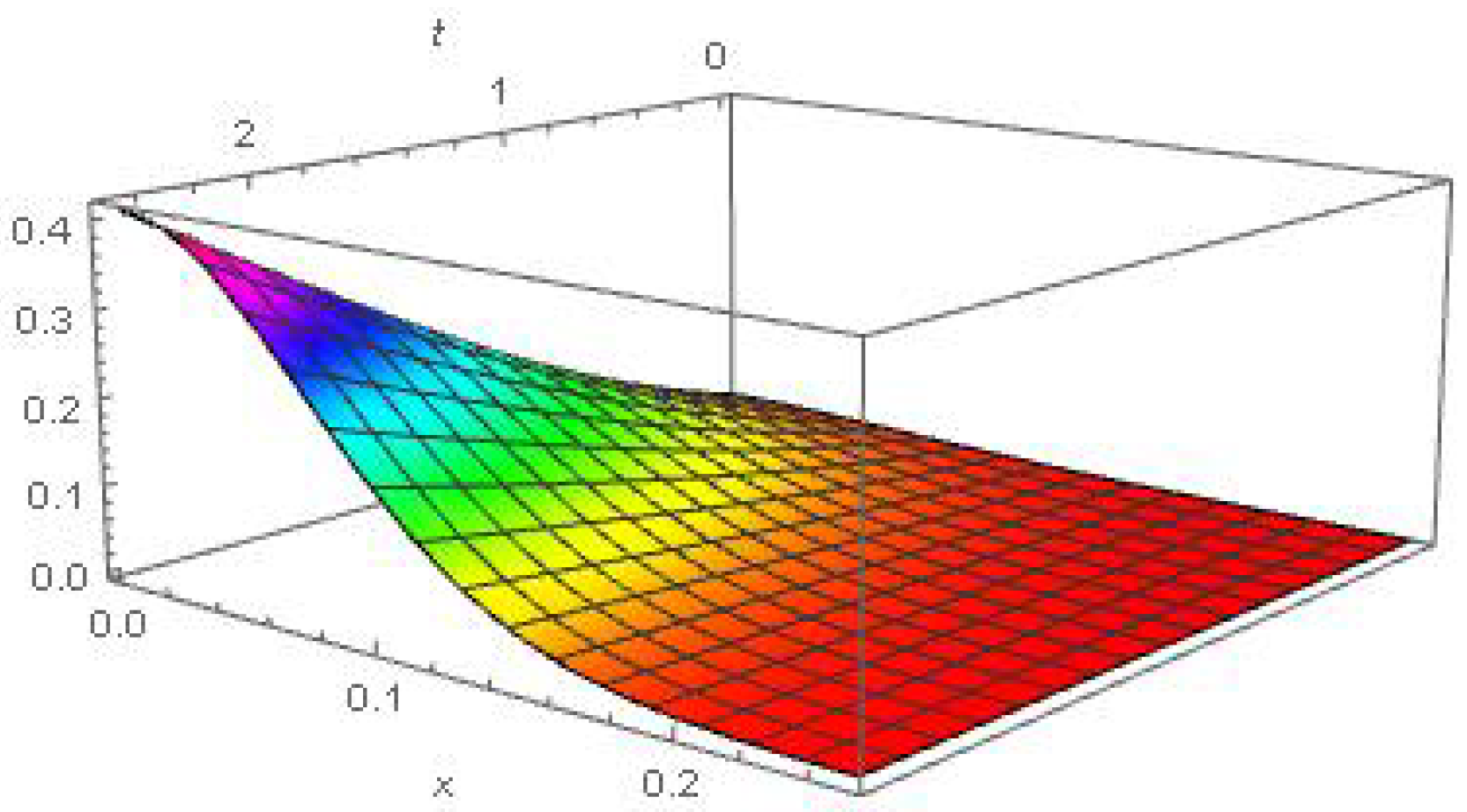
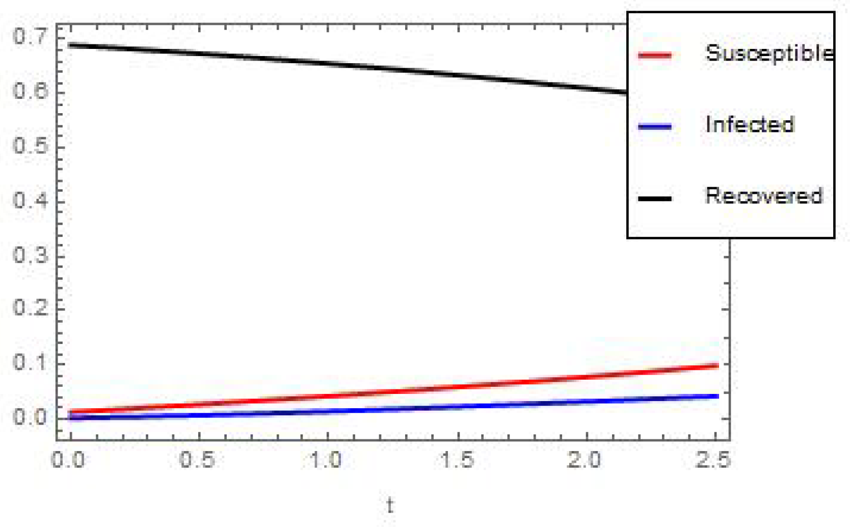
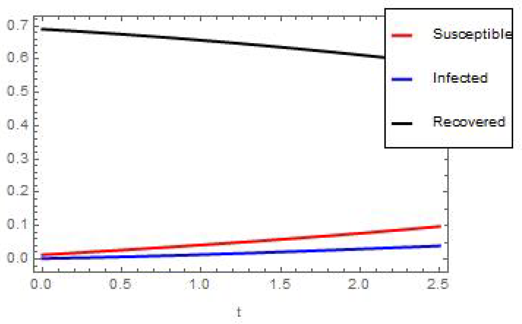
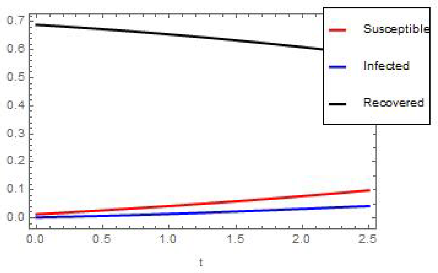
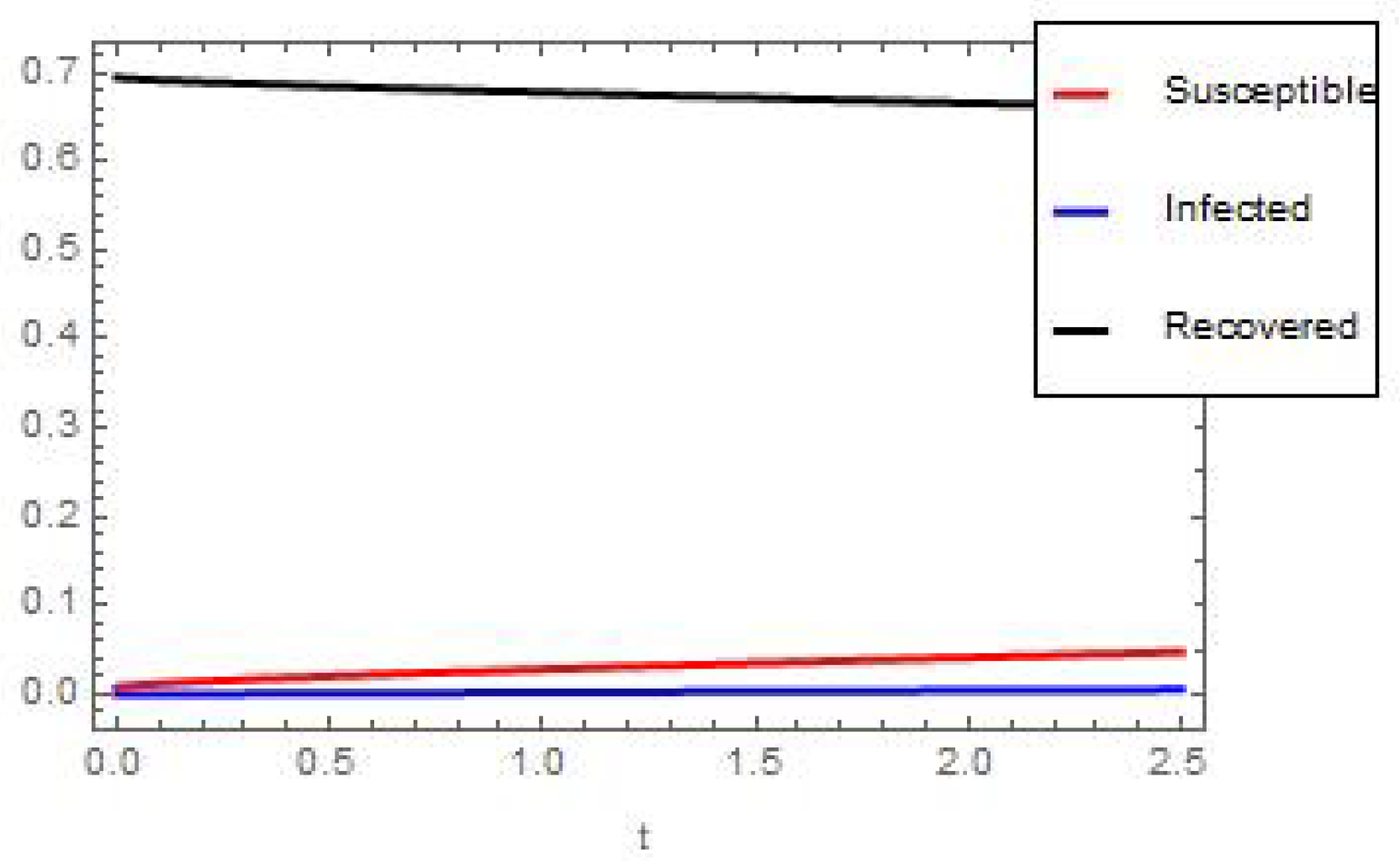
Using the above mentioned values of parameters, along with c 1 = 0.0009 , c 2 = 0.0004 and c 3 = 0.7 in the mathematical results found in the previous section, for time to be fixed as 0 t 2.5 , we can plot the graphs in each case for various factors:
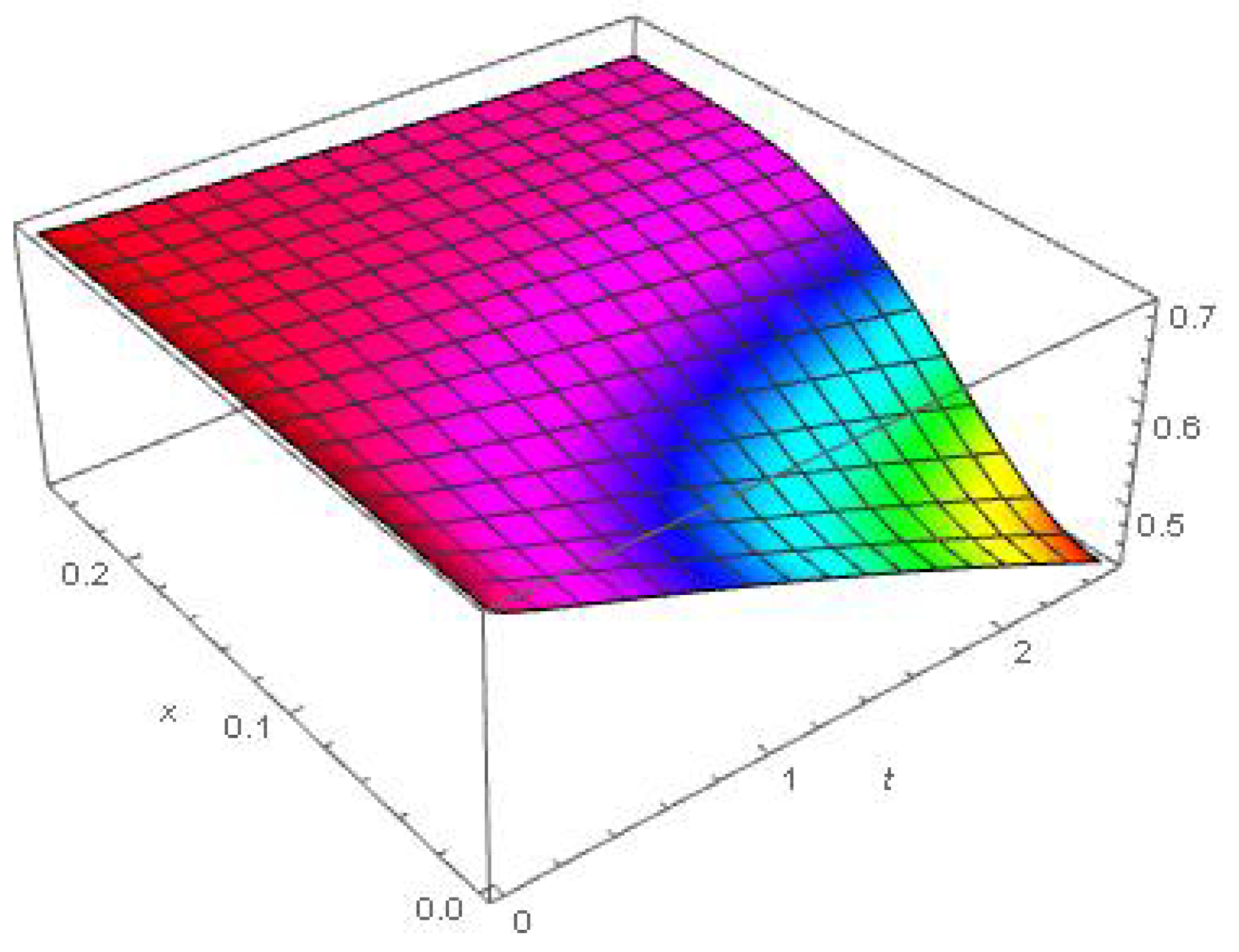
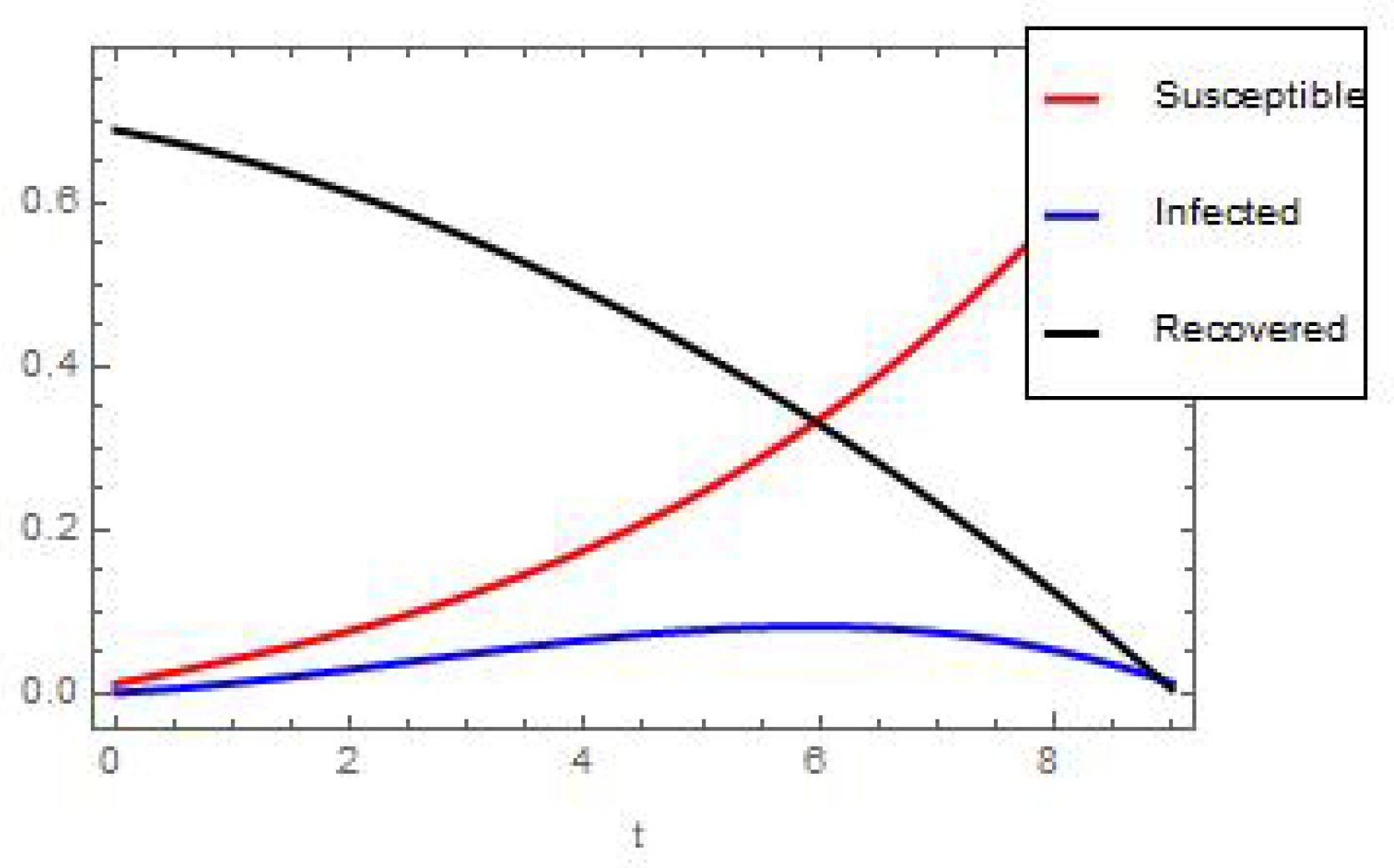
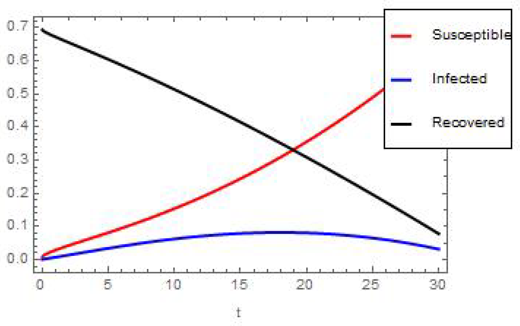
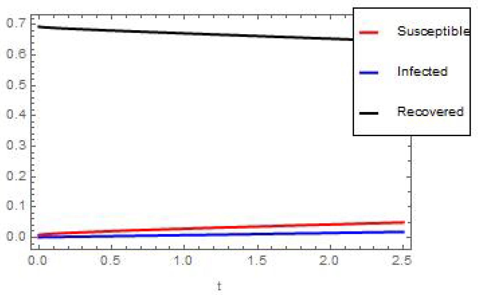
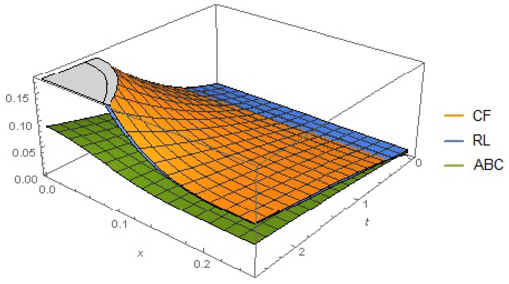
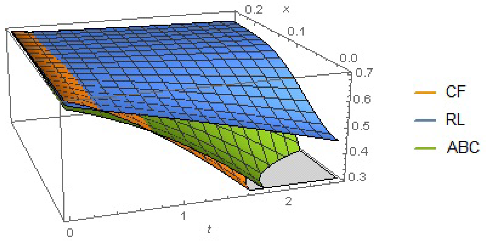
From graphs, we can see that there is a significant impact of the diffusion coefficient of each variable (i.e., susceptible, infected and recovered classes) (Figure 1, Figure 2, Figure 3, Figure 4, Figure 5, Figure 6, Figure 7, Figure 8, Figure 9, Figure 10, Figure 11, Figure 12 and Figure 13). From Figure 13, Figure 14, Figure 15, Figure 16, Figure 17, Figure 18, Figure 19, Figure 20 and Figure 21, we can see that infection is going down as we increase the diffusion coefficient in all the cases. Figure 1, Figure 2, Figure 3, Figure 4, Figure 5, Figure 6, Figure 7, Figure 8 and Figure 9 show the changes in various factors for τ = 0.7 , while Figure 10, Figure 11 and Figure 12 show changes in S, I and in R for x = 0.15, α = 0.001 and τ = 0.7 . In Figure 22, Figure 23 and Figure 24, we see an interesting outcome that the Atangana–Baleanu derivative is showing the lowest peak as compared to other two, when discussing the susceptible and infected class, while in recovery, the Riemann–Liouville derivative is showing better results than the other two. Since we have used the presented model with a unique approach, the presented results are better than the results of [1].

7. Conclusions

In this study, we analyzed the fractional ordered SIR model under the general fractional derivative using the Laplace transform approach. The presence and uniqueness of outcomes were examined using the fixed point method. Once more, the general derivative technique was used to obtain some numerical results for the suggested model. For various fractional orders and for every general derivative scenario, numerical results have been illustrated. By displaying the relationship between two numbers, the graphical depiction demonstrates the greater significance of the fractional order analysis of mathematical models than integer order analysis. As we all know that there is limited predication available for integer ordered derivatives compared to fractional ordered derivatives, in which we can have a large amount of observations available between two integer points. There may also be significant differences in the susceptible, infected and recovered populations when we change the diffusion coefficient and equation’s order.
Now, if we talk about the future research or extending work, then we can also analyze the presented model with the reproduction number, which will certainly give some new and valuable findings for the presented model. There are vast and numerous possibilities in epidemiological modeling using fractional derivatives over integer ordered derivatives, and this will certainly allow for better forecasting and prediction to take more precise corrective steps in the context of real-world situations.

Author Contributions

This study was directed by M.N.M., who also carried out all the mathematical computations. I.A. constructed the study map. R.S.D. summarised the data into tables and drew the figures/graphs. B.S.A. formatted the final paper. The draft was read, corrected and polished by all the authors. All authors have read and agreed to the published version of the manuscript.

Funding

This work was supported and funded by the Deanship of Scientific Research at Imam Mohammad Ibn Saud Islamic University (IMSIU) (grant number IMSIU-RP23002).

Data Availability Statement

Availability of statistics and materials: Availability of statistics is already cited in the article.

Acknowledgments

Authors extend their gratitude to all the reviewers whose suggestations helped to uplift the quality of the article.

Conflicts of Interest

The authors declare no conflicts of interest.

References

  1. Asif, M.; Jan, S.U.; Haider, N.; Al-Mdallal, Q.; Abdeljawad, T. Numerical modeling of npz and sir models with and without diffusion. Results Phys. 2020, 19, 103512. [Google Scholar] [CrossRef]
  2. Asif, M.; Khan, Z.A.; Haider, N.; Al-Mdallal, Q. Numerical simulation for solution of SEIR models by meshless and finite difference methods. Chaos Solitons Fractals 2020, 141, 110340. [Google Scholar] [CrossRef]
  3. Ahmed, N.; Ali, M.; Rafiq, M.; Khan, I.; Nisar, K.S.; Rehman, M.A.; Ahmad, M.O. A numerical efficient splitting method for the solution of two dimensional susceptible infected recovered epidemic model of whooping cough dynamics: Applications in bio-medical engineering. Comput. Methods Programs Biomed. 2020, 190, 105350. [Google Scholar] [CrossRef] [PubMed]
  4. Ergen, K.; Çilli, A.; Yahnıoğlu, N. Predicting epidemic diseases using mathematical modelling of SIR. Acta Phys. Pol. 2015, 128. [Google Scholar] [CrossRef]
  5. Alqarni, M.M.; Nasir, A.; Alyami, M.A.; Raza, A.; Awrejcewicz, J.; Rafiq, M.; Ahmed, N.; Shaikh, T.S.; Mahmoud, E.E. A SEIR Epidemic Model of Whooping Cough-Like Infections and Its Dynamically Consistent Approximation. Complexity 2022, 2022, 3642444. [Google Scholar] [CrossRef]
  6. González-Parra, G.; Arenas, A.J.; Chen-Charpentier, B.M. Combination of nonstandard schemes and Richardson’s extrapolation to improve the numerical solution of population models. Math. Comput. Model. 2010, 52, 1030–1036. [Google Scholar] [CrossRef]
  7. Dang, Q.A.; Hoang, M.T. Nonstandard finite difference schemes for a general predator–prey system. J. Comput. Sci. 2019, 36, 101015. [Google Scholar] [CrossRef]
  8. Kilbas, A.A.; Srivastava, H.M.; Trujillo, J.J. Theory and Applications of Fractional Differential Equations; Elsevier: Amsterdam, The Netherlands, 2006. [Google Scholar]
  9. Koca, I. Analysis of rubella disease model with non-local and non-singular fractional derivatives. Int. J. Optim. Control. Theor. Appl. (IJOCTA) 2018, 8, 17–25. [Google Scholar] [CrossRef]
  10. Yavuz, M.; Özdemir, N. Analysis of an epidemic spreading model with exponential decay law. Math. Sci. Appl.-Notes 2020, 8, 142–154. [Google Scholar] [CrossRef]
  11. Caputo, M.; Fabrizio, M. A new definition of fractional derivative without singular kernel. Prog. Fract. Differ. Appl. 2015, 1, 73–85. [Google Scholar]
  12. Yadav, S.K.; Purohit, M.; Gour, M.M.; Yadav, L.K.; Mishra, M.N. Hybrid technique for multi-dimensional fractional diffusion problems involving Caputo–Fabrizio derivative. Int. J. Math. Ind. 2024, 2450020. [Google Scholar] [CrossRef]
  13. El-Dessoky, M.M.; Khan, M.A. Modeling and analysis of an epidemic model with fractal-fractional Atangana-Baleanu derivative. Alex. Eng. J. 2022, 61, 729–746. [Google Scholar] [CrossRef]
  14. Khan, M.A.; Ullah, S.; Kumar, S. A robust study on 2019-nCOV outbreaks through non-singular derivative. Eur. Phys. J. Plus. 2021, 136, 1–20. [Google Scholar] [CrossRef] [PubMed]
  15. Alazman, I.; Mishra, M.N.; Alkahtani, B.S.; Goswami, P. Computational analysis of rabies and its solution by applying fractional operator. Appl. Math. Sci. Eng. 2024, 32, 2340607. [Google Scholar] [CrossRef]
  16. Owolabi, K.M.; Atangana, A. Mathematical modelling and analysis of fractional epidemic models using derivative with exponential kernel. In Fractional Calculus in Medical and Health Science; CRC Press: Boca Raton, FL, USA, 2020; pp. 109–128. [Google Scholar]
  17. Nisar, K.S.; Farman, M.; Abdel-Aty, M.; Cao, J. A review on epidemic models in sight of fractional calculus. Alex. Eng. J. 2023, 75, 81–113. [Google Scholar] [CrossRef]
  18. Djennadi, S.; Shawagfeh, N.; Osman, M.S.; Gómez-Aguilar, J.F.; Arqub, O.A. The Tikhonov regularization method for the inverse source problem of time fractional heat equation in the view of ABC-fractional technique. Phys. Scr. 2021, 96, 094006. [Google Scholar] [CrossRef]
  19. Alzahrani, E.O.; Khan, M.A. Comparison of numerical techniques for the solution of a fractional epidemic model. Eur. Phys. J. Plus 2020, 135, 110. [Google Scholar] [CrossRef]
  20. Dhandapani, P.B.; Thippan, J.; Baleanu, D.; Sivakumar, V. On a novel fuzzy fractional retarded delay epidemic model. AIMS Math. 2022, 7, 10122–10142. [Google Scholar] [CrossRef]
  21. Areshi, M.; Goswami, P.; Mishra, M.N. Comparative study of blood sugar–insulin model using fractional derivatives. J. Taibah Univ. Sci. 2024, 18, 2339009. [Google Scholar] [CrossRef]
  22. Taghvaei, A.; Georgiou, T.T.; Norton, L.; Tannenbaum, A. Fractional SIR epidemiological models. Sci. Rep. 2020, 10, 20882. [Google Scholar] [CrossRef]
  23. Dubey, R.S.; Mishra, M.N.; Goswami, P. Systematic Analysis of Oxygen Diffusion Problem having Local Fractional Derivative.
  24. Baleanu, D.; Mohammadi, H.; Rezapour, S. Analysis of the model of HIV-1 infection of CD4+ T-cell with a new approach of fractional derivative. Adv. Differ. Equations 2020, 2020, 71. [Google Scholar] [CrossRef]
  25. Kumawat, N.; Shukla, A.; Mishra, M.N.; Sharma, R.; Dubey, R.S. Khalouta Transform and Applications to Caputo-Fractional Differential Equations. Front. Appl. Math. Stat. 2024, 10, 1351526. [Google Scholar] [CrossRef]
  26. Liu, X.; ur Rahmamn, M.; Ahmad, S.; Baleanu, D.; Nadeem Anjam, Y. A new fractional infectious disease model under the non-singular Mittag–Leffler derivative. Waves Random Complex Media 2022, 1–27. [Google Scholar] [CrossRef]
  27. Yang, X.J.; Baleanu, D.; Srivastava, H.M. Local Fractional Integral Transforms and Their Applications; Academic Press: Cambridge, MA, USA, 2015. [Google Scholar]
  28. Alazman, I.; Alkahtani, B.S.T.; Rahman, M.U.; Mishra, M.N. Nonlinear complex dynamical analysis and solitary waves for the (3+1)-D nonlinear extended Quantum Zakharov–Kuznetsov equation. Results Phys. 2024, 58, 107432. [Google Scholar] [CrossRef]
  29. Ammi, M.R.S.; Tahiri, M.; Torres, D.F. Necessary optimality conditions of a reaction-diffusion SIR model with ABC fractional derivatives. arXiv 2021, arXiv:2106.15055. [Google Scholar] [CrossRef]
  30. Losada, J.; Nieto, J.J. Properties of a new fractional derivative without singular kernel. Progr. Fract. Differ. Appl 2015, 1, 87–92. [Google Scholar]
  31. Zhenzhen, L.; Yongguang, Y.; Weiyi, X.; Guojian, R.; Xiangyun, M. Global dynamics for a class of discrete fractional epidemic model with reaction-diffusion. arXiv 2022, arXiv:2208.06548. [Google Scholar]
  32. Sidi Ammi, M.R.; Tahiri, M.; Tilioua, M.; Zeb, A.; Khan, I.; Andualem, M. Global analysis of a time fractional order spatio-temporal SIR model. Sci. Rep. 2022, 12, 5751. [Google Scholar] [CrossRef]
  33. İlhan, Ö.; Şahin, G. A numerical approach for an epidemic SIR model via Morgan-Voyce series. Int. J. Math. Comput. Eng. 2024, 2, 125–140. [Google Scholar] [CrossRef]
  34. Kumar, M.; Jhinga, A.; Daftardar-Gejji, V. New algorithm for solving non-linear functional equations. Int. J. Appl. Comput. Math. 2020, 6, 26. [Google Scholar] [CrossRef]
  35. Daftardar-Gejji, V.; Jafari, H. An iterative method for solving nonlinear functional equations. J. Math. Anal. Appl. 2006, 316, 753–763. [Google Scholar] [CrossRef]
  36. Angstmann, C.N.; Henry, B.I.; McGann, A.V. A fractional-order infectivity and recovery SIR model. Fractal Fract. 2017, 1, 11. [Google Scholar] [CrossRef]
  37. Alòs, E.; Mancino, M.E.; Merino, R.; Sanfelici, S. A fractional model for the COVID-19 pandemic: Application to Italian data. Stoch. Anal. Appl. 2021, 39, 842–860. [Google Scholar] [CrossRef]
  38. Angstmann, C.N.; Henry, B.I.; McGann, A.V. A fractional-order infectivity SIR model. Phys. A Stat. Mech. Appl. 2016, 452, 86–93. [Google Scholar] [CrossRef]
  39. Singh, A.K.; Mehra, M.; Gulyani, S. A modified variable-order fractional SIR model to predict the spread of COVID-19 in India. Math. Methods Appl. Sci. 2023, 46, 8208–8222. [Google Scholar] [CrossRef]
  40. Singh, R.; Mishra, J.; Gupta, V.K. Dynamical analysis of a Tumor Growth model under the effect of fractal fractional Caputo-Fabrizio derivative. Int. J. Math. Comput. Eng. 2023, 1, 115–126. [Google Scholar] [CrossRef]
  41. Agarwal, H.; Mishra, M.N.; Dubey, R.S. On fractional Caputo operator for the generalized glucose supply model via incomplete Aleph function. Int. J. Math. Ind. 2024, 2024, 2450003. [Google Scholar] [CrossRef]
  42. Alqahtani, A.M.; Mishra, M.N. Mathematical Analysis of Streptococcus Suis Infection in Pig- Human Population by Riemann-Liouville Fractional Operator. Prog. Fract. Differ. Appl. 2024, 10, 119–135. [Google Scholar]
  43. Sabir, Z.; Umar, M. Levenberg-Marquardt backpropagation neural network procedures for the consumption of hard water-based kidney function. Int. J. Math. Comput. Eng. 2023, 1, 127–138. [Google Scholar] [CrossRef]
  44. Alqahtani, A.M.; Shukla, A. Computational analysis of multi-layered Navier–Stokes system by Atangana–Baleanu derivative. Appl. Math. Sci. Eng. 2024, 32, 2290723. [Google Scholar] [CrossRef]
  45. Moore, E.J.; Sirisubtawee, S.; Koonprasert, S. A Caputo–Fabrizio fractional differential equation model for HIV/AIDS with treatment compartment. Adv. Differ. Equ. 2019, 2019, 200. [Google Scholar] [CrossRef]
  46. Luchko, Y.; Yamamoto, M. General time-fractional diffusion equation: Some uniqueness and existence results for the initial-boundary-value problems. Fract. Calc. Appl. Anal. 2016, 19, 676–695. [Google Scholar] [CrossRef]
  47. Yasin, M.W.; Ahmed, N.; Iqbal, M.S.; Rafiq, M.; Raza, A.; Akgül, A. Reliable numerical analysis for stochastic reaction-diffusion system. Phys. Scr. 2022, 98, 015209. [Google Scholar] [CrossRef]
  48. Phaijoo, G.R.; Gurung, D.B. Sensitivity analysis of SEIR-SEI model of dengue disease. Gams J. Math. Math. Biosci. 2018, 6, 41–50. [Google Scholar]
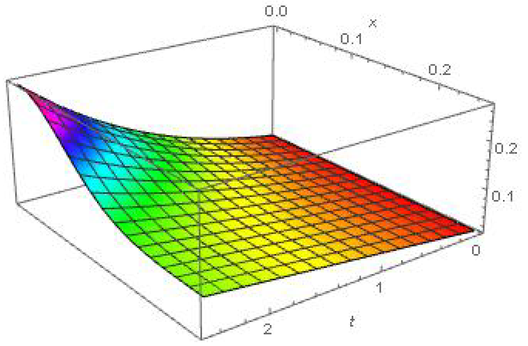
Figure 1. Graph of susceptible against time t, for τ = 0.7 and α = 0.001 in Caputo–Fabrizio case.
Fractalfract 08 00537 g001
Figure 2. Graph of infected against time t, for τ = 0.7 and α = 0.001 in Caputo–Fabrizio case.
Fractalfract 08 00537 g002
Figure 3. Graph of recovered against time t, for τ = 0.7 and α = 0.001 in Caputo–Fabrizio case.
Fractalfract 08 00537 g003
Figure 4. Graph of susceptible with respect to t, for τ = 0.7 and α = 0.001 in Riemann–Liouville’s case.
Fractalfract 08 00537 g004
Figure 5. Graph of infected with respect to t, for τ = 0.7 and α = 0.001 in Riemann–Liouville’s case.
Fractalfract 08 00537 g005
Figure 6. Graph of recovered with respect to t, for τ = 0.7 and α = 0.001 in Riemann–Liouville’s case.
Fractalfract 08 00537 g006
Figure 7. Graph of susceptible with respect to t, for τ = 0.7 and α = 0.001 in ABC case.
Fractalfract 08 00537 g007
Figure 8. Graph of infected with respect to t, for τ = 0.7 and α = 0.001 in ABC case.
Fractalfract 08 00537 g008
Figure 9. Graph of recovered with respect to t, for τ = 0.7 and α = 0.001 in ABC case.
Fractalfract 08 00537 g009
Figure 10. Graph of susceptible, infected and recovered class with respect to t, for x=0.15, α = 0.001 and τ = 0.7 in CF case.
Fractalfract 08 00537 g010
Figure 11. Graph of susceptible, infected and recovered class with respect to t, for x=0.15, α = 0.001 and τ = 0.7 in RL case.
Fractalfract 08 00537 g011
Figure 12. Graph of susceptible, infected and recovered class with respect to t, for x=0.15, α = 0.001 and τ = 0.7 in ABC case.
Fractalfract 08 00537 g012
Figure 13. Graph of susceptible, infected and recovered class with respect to t, for diffusion coefficient 0.01 in CF case.
Fractalfract 08 00537 g013
Figure 14. Graph of susceptible, infected and recovered class with respect to t, for diffusion coefficient 0.001 in CF case.
Fractalfract 08 00537 g014
Figure 15. Graph of susceptible, infected and recovered class with respect to t, for diffusion coefficient 0.0001 in CF case.
Fractalfract 08 00537 g015
Figure 16. Graph of susceptible, infected and recovered class with respect to t, for diffusion coefficient 0.01 in RL case.
Fractalfract 08 00537 g016
Figure 17. Graph of susceptible, infected and recovered class with respect to t, for diffusion coefficient 0.001 in RL case.
Fractalfract 08 00537 g017
Figure 18. Graph of susceptible, infected and recovered class with respect to t, for diffusion coefficient 0.0001 in RL case.
Fractalfract 08 00537 g018
Figure 19. Graph of susceptible, infected and recovered class with respect to t, for diffusion coefficient 0.01 in ABC case.
Fractalfract 08 00537 g019
Figure 20. Graph of susceptible, infected and recovered class with respect to t, for diffusion coefficient 0.001 in ABC case.
Fractalfract 08 00537 g020
Figure 21. Graph of susceptible, infected and recovered class with respect to t, for diffusion coefficient 0.0001 in ABC case.
Fractalfract 08 00537 g021
Figure 22. Graph of susceptible with CF, RL and ABC derivative for τ = 0.7 and α = 0.001 .
Fractalfract 08 00537 g022
Figure 23. Graph of infected with CF, RL and ABC derivative for τ = 0.7 and α = 0.001 .
Fractalfract 08 00537 g023
Figure 24. Graph of recovered with CF, RL and ABC derivative for τ = 0.7 and α = 0.001 .
Fractalfract 08 00537 g024
Table 1. Table of parameters used.
S.N.VariableSymbolValue
1Birth rate μ 0.04
2Recovery rate ν 24
3Transmission rate γ 123
Disclaimer/Publisher’s Note: The statements, opinions and data contained in all publications are solely those of the individual author(s) and contributor(s) and not of MDPI and/or the editor(s). MDPI and/or the editor(s) disclaim responsibility for any injury to people or property resulting from any ideas, methods, instructions or products referred to in the content.