Feedback Control Design Strategy for Stabilization of Delayed Descriptor Fractional Neutral Systems with Order 0 < ϱ < 1 in the Presence of Time-Varying Parametric Uncertainty

Abstract

Descriptor systems are more complex than normal systems, which are modeled by differential equations. This paper derives stability and stabilization criteria for uncertain fractional descriptor systems with neutral-type delay. Through the Lyapunov–Krasovskii functional approach, conditions subject to time-varying delay and parametric uncertainty are formulated as linear matrix inequalities. Based on the established criteria, static state- and output-feedback control laws are designed to ensure regularity and impulse-free properties, together with robust stability of the closed-loop system under permissible uncertainties. Numerical examples illustrate the effectiveness of the control methods and show that the results depend on the range of variation in the delays and on the fractional order, leading to stability analysis results that are less conservative than those reported in the literature.

1. Introduction

Nowadays, descriptor systems (DSs), or singular systems, are considered an interesting research topic due to their broad applications in the fields of economics, robotics, and electrical circuit networks [1,2,3,4], just to mention a few. The DSs are described as a set of coupled algebraic/differential equations, involving both static and dynamic constraints [1], which are able to accurately model a variety of physical phenomena encountered in real-world plants [5]. Due to their ability to describe impulsive characteristics and non-dynamic constraints, the stability and stabilization of DSs have gained much attention in control theory [6,7,8]. Indeed, from this perspective, the stabilization of DSs presents a problem much more demanding than that involving other systems.

In the real-world, we face time delay as an inevitable phenomenon, which often causes poor system’s behavior and instability. Therefore, it is necessary to design appropriate controllers to stabilize systems with time delays [9,10,11]. Neutral-type systems are a class of delayed systems that include delays in their states and states’ derivatives [12]. They often appear in control processes [13], partial element equivalent circuits [14], network-based control systems [15], and population ecology [16], among others. The neutral-type delay DSs have received attention in recent years [17,18,19].

Fractional calculus is a field of applied mathematics, which emerged and gained relevance in almost every branch of science, engineering and mathematics [20,21,22,23,24,25]. Fractional-order (FO) models, that is, those that include FO differential and integral operators, can describe heterogeneity and, therefore, the dynamic behavior of complex systems, more accurately than traditional integer-order (IO) models [26,27]. Besides modeling, applications of fractional calculus in systems’ identification [28], signal [29] and image processing [30], and control systems design [31,32,33], are also common. Nonetheless, FO systems, meaning those described by means of FO models, are more complex than IO systems [34]. Thus, the study of FO systems emerged as an interesting and challenging topic [35], namely concerning their stability and stabilization problems [36,37]. In reference [38], the stabilization of delayed memristor neural networks of FO was investigated. In the work [39], the finite-time stability of delayed impulsive systems of FO was discussed. The fractional DSs (FDSs) are a type of FO system with specific dynamic characteristics. Therefore, the extension of general systems’ concepts, such as observability, controllability and stability [40,41] to the FDSs presents a challenging research topic. Recently, DSs received attention in modeling applications, such as in robotics [42], economics [43], and power systems [44].

Stability is crucial in control systems design [45]. Different works on the stability of IO and FO systems can be found in the literature, based on linear matrix inequalities (LMIs) [46]. Although stability of integer DSs (IDSs) has been well addressed, we can find just a few articles focusing on FDSs, and even less for FDSs with time delay. A key problem in delayed FDSs is the effect of delay on the impulsivity and regularity properties of DSs. Thus, the stability analysis of delayed IDSs and FDSs is an important topic. In reference [47], the robust stability of delayed IDSs was investigated. In the works [18,48], the stability of neutral-type delay IDSs was addressed via the Lyapunov–Krasovskii (L-K) functional method. In references [49,50], the asymptotic stability of continuous and discrete FDSs with time delay were discussed, respectively. In the works [51,52], the stability of stochastic and positive FDSs with time delay were addressed, respectively. Nevertheless, the time delay effect on the stability of FDSs was not properly tackled in the aforementioned works, in particular for the neutral-type case, which is more complex than other kinds of delays.

To the best of the authors’ knowledge, the stabilization of uncertain FDSs under varying delay has not yet been entirely addressed in the literature. Specifically, for FDSs of time-varying neutral type, no studies were reported, and thus the topic still remains challenging. In this paper, the robust stabilization of uncertain FDSs considering time-varying neutral-type delay is addressed. Adopting the L-K functional technique, LMI-based criteria are derived to achieve asymptotic robust stability. Proper static state- and output-feedback control laws are derived for system’s stabilization. Numerical examples are provided to illustrate the effectiveness of the theoretical findings.

The main contributions are:

•

The L-K functional technique is adopted to study the asymptotical stability of FDSs with neutral-type delay subject to time-varying delays and parametric uncertainties.

•

Static state- and output-feedback controllers are designed to ensure regularity and impulse-free properties together, and delay-dependent and order-dependent conditions are achieved in the form of LMIs for the existence of such controllers.

The structure of the paper is as follows. Section 2 and Section 3 give the theoretical background and the statement of the problem in hand, respectively. Section 4 and Section 5 present LMI-based stability and control design conditions of the FDSs with time-varying neutral-type delay. Section 6 provides simulations results to verify the capabilities of the proposed method. Finally, Section 7 outlines the conclusions.

2. Theoretical Background

A few notes about the used notation are given in the follow-up. The transpose and the inverse of a matrix Z are denoted by $Z^T$ and $Z^{-1}$, respectively. The symbol $\mathrm{deg}\left(\mathfrak{f}\right(\sigma \left)\right)$ is used for the degree of the polynomial $\mathfrak{f}\left(\sigma \right)$, $\det \left(Z\right)$ denotes the determinant of the matrix Z, I stands for the identity matrix with compatible size, ${\mathfrak{R}}^m$ and ${\mathfrak{R}}^{m\times n}$ denote the m-dimensional Euclidean space and the set of $m\times n$ matrices, respectively, $P\le 0(P<0)$ stands for a negative semi-definite (negative definite) matrix, $P\ge 0(>0)$ denotes a positive semi-definite (positive definite) matrix, and the symbol ∗ is used to represent symmetric elements of any symmetric matrix.

There are different definitions of FO derivative, namely the Caputo, the Riemann–Liouville, and the Grünwald–Letnikov ones. Due to the Caputo derivative suitability for describing initial value FO problems, we adopt this formulation in this article. The Caputo derivative of a continuous function $\upsilon \left(t\right)$ with FO $\varrho$, is given by [53]

$${\mathfrak{D}}_t^{\varrho }\upsilon \left(t\right)={\displaystyle \frac{1}{\Gamma (1-\varrho )}}\underset{0}{\overset{t}{\int }}{\left(t-\theta \right)}^{-\varrho }{\upsilon }^{\prime }\left(\theta \right)\mathrm{d}\theta ,$$

(1)

where $\Gamma \left(\sigma \right)={\int }_0^{\infty }{t}^{\sigma -1}{e}^{-t}\mathrm{d}t$ and $0<\varrho <1$.

Lemma 1 

([54]). For a real matrix $\Lambda ={\Lambda }^T$, the following conditions hold

$$\begin{array}{cc}\hfill & \Lambda =\left(\begin{array}{cc}{\Lambda }_{11}& {\Lambda }_{12}\\ \ast & {\Lambda }_{22}\end{array}\right)<0,\hfill \\ \hfill & {\Lambda }_{11}<0,{\Lambda }_{22}-{{\Lambda }_{12}}^T{{\Lambda }_{11}}^{-1}{\Lambda }_{12}<0,\hfill \\ \hfill & {\Lambda }_{22}<0,{\Lambda }_{11}-{\Lambda }_{12}{{\Lambda }_{22}}^{-1}{{\Lambda }_{12}}^T<0.\hfill \end{array}$$

(2)

Lemma 2 

([55,56]). For the matrix $\Pi \in {\mathfrak{R}}^{n\times n}>0$, we have

$$0.5{\mathfrak{D}}_t^{\varrho }\left({\chi }^T\left(t\right)\Pi \chi \left(t\right)\right)\le {\chi }^T\left(t\right)\Pi \left({\mathfrak{D}}_t^{\varrho }\chi \left(t\right)\right),\varrho \in \left(0,1\right),$$

(3)

where the vector-valued function $\chi \left(t\right)\in {\mathfrak{R}}^n$ is differentiable.

Lemma 3 

([57]). For $\mathcal{G}\left(t\right)$, with ${\mathcal{G}}^T\left(t\right)\mathcal{G}\left(t\right)\le I$, and the real matrices $\mathcal{F},\mathcal{N}$ and $\mathcal{H}$, with compatible sizes, we have

$$\mathcal{F}+\mathcal{N}\mathcal{G}\left(t\right)\mathcal{H}+{\mathcal{H}}^T{\mathcal{G}}^T\left(t\right){\mathcal{N}}^T<0,$$

(4)

if and only if a scalar $\kappa >0$ exists, such that

$$\kappa \mathcal{N}{\mathcal{N}}^T+{\kappa }^{-1}{\mathcal{H}}^T\mathcal{H}+\mathcal{F}<0.$$

(5)

3. Formulation of the Problem

Let us consider the uncertain FDS with neutral-type varying delay:

$$\begin{array}{cc}\hfill E{\mathfrak{D}}_t^{\varrho }\upsilon \left(t\right)& ={\mathcal{A}}_0\left(t\right){\mathfrak{D}}_t^{\varrho }\upsilon (t-\mu \left(t\right))+{\mathcal{A}}_d\left(t\right)\upsilon (t-\mu \left(t\right))+\mathcal{A}\left(t\right)\upsilon \left(t\right)+\mathcal{B}u\left(t\right),\hfill \\ \hfill y\left(t\right)& =\mathcal{C}\upsilon \left(t\right),\hfill \\ \hfill \upsilon \left(t\right)& =\psi \left(t\right),t\in [-{\mu }_m,0],\hfill \end{array}$$

(6)

where $\upsilon \in {\mathfrak{R}}^n$, $u\in {\mathfrak{R}}^m$ and $y\left(t\right)\in {\mathfrak{R}}^l$ represent the state, the input and the output vectors, respectively, ${\mathcal{A}}_d\left(t\right)={\mathcal{A}}_d+\Delta {\mathcal{A}}_d\left(t\right),\mathcal{A}\left(t\right)=\mathcal{A}+\Delta \mathcal{A}\left(t\right)$ and ${\mathcal{A}}_0\left(t\right)={\mathcal{A}}_0+\Delta {\mathcal{A}}_0\left(t\right)$, with ${\mathcal{A}}_d,\mathcal{A}$ and ${\mathcal{A}}_0$, being known constant real matrices with compatible sizes, $\Delta \mathcal{A}\left(t\right),\Delta {\mathcal{A}}_d\left(t\right)$ and $\Delta {\mathcal{A}}_0\left(t\right)$ are uncertainty terms, E denotes a known constant real matrix so that $\mathrm{rank}\left(E\right)=r\le n$, $\mathcal{B}$ and $\mathcal{C}$ are known constant real matrices, and $\mu \left(t\right)$ is the delay. Additionally, $\upsilon \left(t\right)=\psi \left(t\right)$ represents some continuous initial condition.

If $\det (s^{\varrho }E-\mathcal{A})\ne 0$, then the pair $(E,\mathcal{A})$ is regular, where s is an arbitrary constant. Moreover, if $\mathrm{deg}\left[\det (s^{\varrho }E-\mathcal{A})\right]=\mathrm{rank}\left(E\right)$, then $(E,\mathcal{A})$ is impulse-free. If the regularity and impulse-free properties of $(E,\mathcal{A})$ are simultaneously meet, then the pair $(E,\mathcal{A})$ is admissible as well. If for all roots of $\det (s^{\varrho }E-\mathcal{A})=0$ the condition $\left|\arg \left(\mathrm{spec}(E,\mathcal{A})\right)\right|>\varrho {\displaystyle \frac{\pi }{2}}$ holds, where $\mathrm{spec}(E,\mathcal{A})$ denotes the set of all roots of $\det (s^{\varrho }E-\mathcal{A})=0$, then the pair $(E,\mathcal{A})$ is stable [58].

In the following, for the sake of simplicity, we use $\Delta \mathcal{A},\Delta {\mathcal{A}}_d$ and $\Delta {\mathcal{A}}_0$ instead of $\Delta \mathcal{A}\left(t\right),\Delta {\mathcal{A}}_d\left(t\right)$ and $\Delta {\mathcal{A}}_0\left(t\right)$.

General Assumptions and Control Goals

We consider the following assumptions:

• A1: The uncertainty terms satisfy

  $$\begin{array}{c}\hfill \begin{array}{ccc}[\Delta \mathcal{A}& \Delta {\mathcal{A}}_d& \Delta {\mathcal{A}}_0\end{array}]=\mathcal{H}\mathcal{G}\left(t\right)[\begin{array}{ccc}{\mathcal{E}}_0& {\mathcal{E}}_1& {\mathcal{E}}_2],\end{array}\end{array}$$

  (7)

  where the real constant matrices $\mathcal{H}$ and ${\mathcal{E}}_i,i=0,1,2$, are known and have compatible sizes, and the time-varying matrix $\mathcal{G}\left(t\right)$ is real, unknown and satisfies ${\mathcal{G}}^T\left(t\right)\mathcal{G}\left(t\right)\le I$.
• A2: The delay $\mu \left(t\right)$ is continuous with bounded derivative satisfying

  $$0\le \mu \left(t\right)\le {\mu }_m,\dot{\mu }\left(t\right)\le {\mu }^{★},$$

  (8)

  in which ${\mu }_m$ and ${\mu }^{★}<1$ are constants.
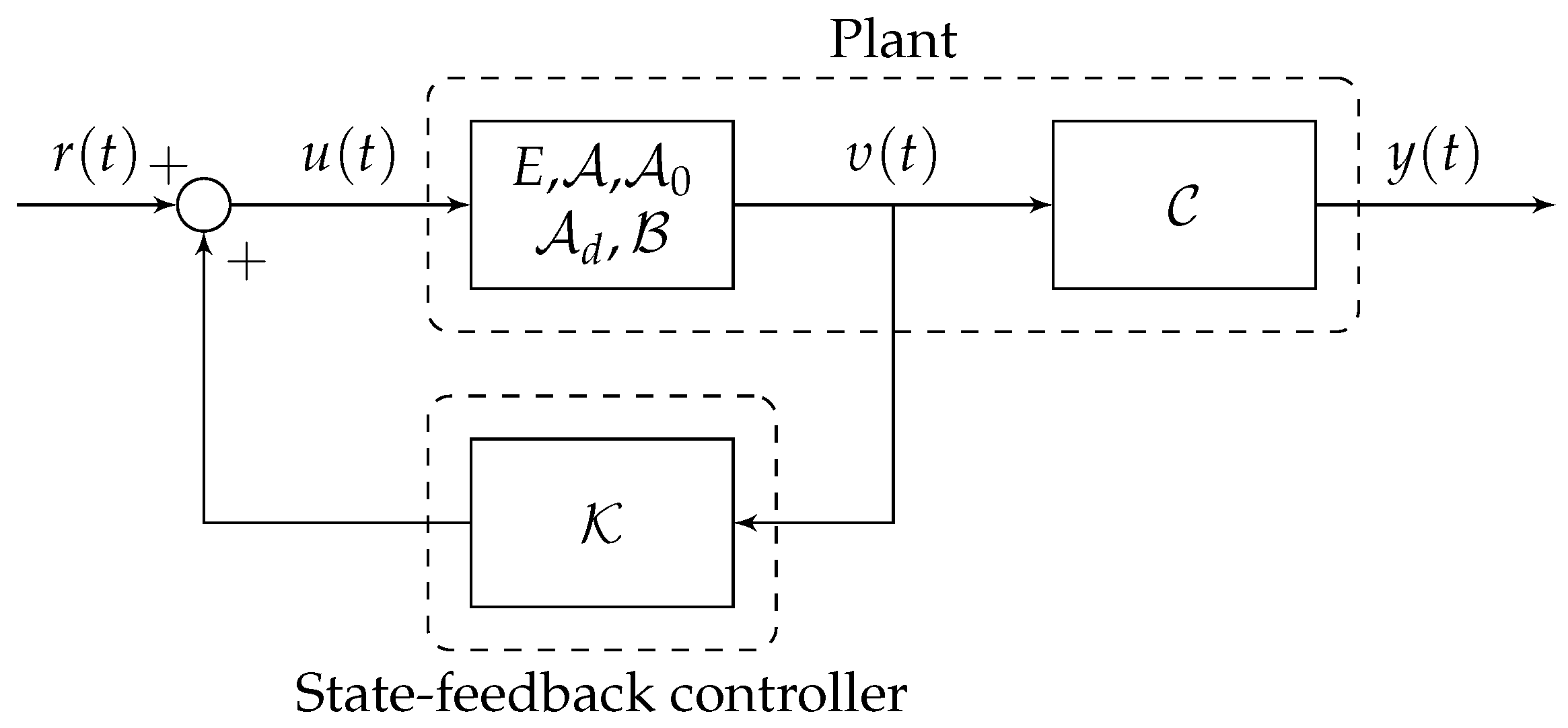
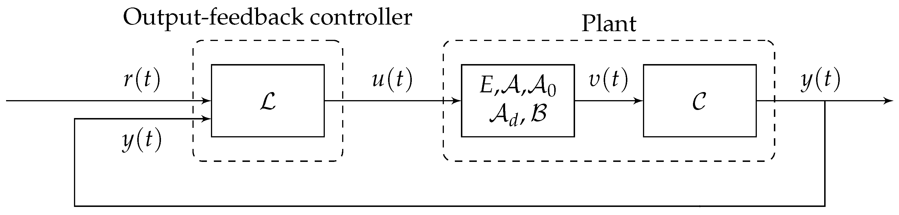
• A3: The static state- and output-feedback techniques are adopted for control, which are given by

  $$\begin{array}{c}\hfill u\left(t\right)=\mathcal{K}\upsilon \left(t\right),\\ \hfill u\left(t\right)=\mathcal{L}y\left(t\right),\end{array}$$

  (9)

  where $\mathcal{K}$ and $\mathcal{L}$ denote the state and output controller gains, respectively, which are computed based on LMI conditions.

In this article, we also consider the following control goals:

• G1: Deriving the sufficient stability and robust stability criteria for the nominal system, that is, $\Delta \mathcal{A}=\Delta {\mathcal{A}}_d=\Delta {\mathcal{A}}_0=0$, and the uncertain system (6), respectively.
• G2: Deriving the sufficient stabilization and robust stabilization of the controlled system by designing an appropriate feedback controller (9).

4. Stability Analysis

Herein, we discuss the stability for the nominal and uncertain FDS (6), separately, with the help of LMIs.

4.1. Nominal Stability

In the follow-up, we present Theorem 1 providing the stability criterion for the nominal FDS (6).

Theorem 1. 

Consider the nominal FDS (6) with the scalars ${\mu }_m$ and $0<\varrho <1$. For the existence of any matrices N and $\mathcal{S}$ with compatible size, positive-definite symmetric matrices $\mathcal{Q},\mathcal{Z}$ and $\mathcal{P}$, and semi positive-definite symmetric matrices $\mathcal{T}$ and $\mathcal{R}$ with compatible dimension so that

$$\left(\begin{array}{ccccc}{\Phi }_{11}& {\Phi }_{12}& {\Phi }_{13}& {\mathcal{A}}^T\mathcal{Z}& {{\mu }_m}^{\varrho }{\varrho }^{-1}{\mathcal{A}}^T\mathcal{T}\\ \ast & -(1-{\mu }^{★})\mathcal{Q}& 0& {{\mathcal{A}}_d}^T\mathcal{Z}& {{\mu }_m}^{\varrho }{\varrho }^{-1}{{\mathcal{A}}_d}^T\mathcal{T}\\ \ast & \ast & -(1-{\mu }^{★})E^T\mathcal{Z}E& {{\mathcal{A}}_0}^T\mathcal{Z}& {{\mu }_m}^{\varrho }{\varrho }^{-1}{{\mathcal{A}}_0}^T\mathcal{T}\\ \ast & \ast & \ast & -\mathcal{Z}& 0\\ \ast & \ast & \ast & \ast & -{{\mu }_m}^{\varrho }{\varrho }^{-1}\mathcal{T}\end{array}\right)<0,$$

(10)

$$\begin{array}{c}\hfill \Lambda =\left(\begin{array}{cc}\mathcal{R}& \mathcal{S}\\ & \mathcal{T}\end{array}\right)\ge 0,\end{array}$$

where

$$\begin{array}{cc}\hfill {\Phi }_{11}& ={\mathcal{A}}^T\mathcal{P}E+E^T\mathcal{P}\mathcal{A}+\mathcal{Q}+{{\mu }_m}^{\varrho }{\varrho }^{-1}({\mathcal{A}}^T{\mathcal{S}}^T+\mathcal{S}\mathcal{A}+\mathcal{R})+{\mathcal{A}}^{T}Y{N}^T+N{Y}^T\mathcal{A},\hfill \\ \hfill {\Phi }_{12}& =E^T\mathcal{P}{\mathcal{A}}_d+{{\mu }_m}^{\varrho }{\varrho }^{-1}\mathcal{S}{\mathcal{A}}_d+N{Y}^T{\mathcal{A}}_d,\hfill \\ \hfill {\Phi }_{13}& =E^T\mathcal{P}{\mathcal{A}}_0+{{\mu }_m}^{\varrho }{\varrho }^{-1}\mathcal{S}{\mathcal{A}}_0+N{Y}^T{\mathcal{A}}_0,\hfill \end{array}$$

and the full column rank matrix $Y\in {\mathfrak{R}}^{n\times (n-r)}$ with $E^{T}Y=0$, the nominal FDS (6) is simultaneous regular, impulse-free and stable.

Proof. 

From $\mathrm{rank}\left(E\right)=r\le n$, it is possible to obtain invertible matrices $F,G\in {\mathfrak{R}}^{n\times n}$ satisfying

$$\overline{E}=GEF=\left(\begin{array}{cc}{I}_r& 0\\ 0& 0\end{array}\right).$$

(11)

Under the condition $E^{T}Y=0$, we can represent Y as $Y=G^T\left(\begin{array}{c}0\\ \overline{\phi }\end{array}\right)$, in which a nonsingular matrix denoted by $\overline{\phi }$ belongs to ${\mathfrak{R}}^{(n-r)\times (n-r)}$. Similarly, we can obtain

$$\begin{array}{cc}\hfill \overline{\mathcal{A}}& =G\mathcal{A}F=\left(\begin{array}{cc}{\overline{\mathcal{A}}}_{11}& {\overline{\mathcal{A}}}_{12}\\ {\overline{\mathcal{A}}}_{21}& {\overline{\mathcal{A}}}_{22}\end{array}\right),\hfill \end{array}$$

(12)

$$\begin{array}{cc}\hfill \overline{\mathcal{P}}& =G^{-T}\mathcal{P}{G}^{-1}=\left(\begin{array}{cc}{\overline{\mathcal{P}}}_{11}& {\overline{\mathcal{P}}}_{12}\\ {\overline{\mathcal{P}}}_{21}& {\overline{\mathcal{P}}}_{22}\end{array}\right),\hfill \end{array}$$

(13)

$$\begin{array}{cc}\hfill \overline{\mathcal{S}}& =G^{-T}\mathcal{S}F=\left(\begin{array}{cc}{\overline{\mathcal{S}}}_{11}& {\overline{\mathcal{S}}}_{12}\\ {\overline{\mathcal{S}}}_{21}& {\overline{\mathcal{S}}}_{22}\end{array}\right),\hfill \end{array}$$

(14)

$$\begin{array}{cc}\hfill \overline{\mathcal{R}}& =G^{-T}\mathcal{R}F=\left(\begin{array}{cc}{\overline{\mathcal{R}}}_{11}& {\overline{\mathcal{R}}}_{12}\\ {\overline{\mathcal{R}}}_{21}& {\overline{\mathcal{R}}}_{22}\end{array}\right),\hfill \end{array}$$

(15)

$$\begin{array}{cc}\hfill \overline{N}& =F^{T}N=\left(\begin{array}{c}{\overline{N}}_{11}\\ {\overline{N}}_{21}\end{array}\right),\hfill \end{array}$$

(16)

$$\begin{array}{cc}\hfill \overline{Y}& =G^{-T}Y=\left(\begin{array}{c}0\\ \overline{\phi }\end{array}\right).\hfill \end{array}$$

(17)

From ${\Phi }_{11}<0$ and $\mathcal{Q}>0$, we have

$${\mathcal{A}}^T\mathcal{P}E+E^T\mathcal{P}\mathcal{A}+{{\mu }_m}^{\varrho }{\varrho }^{-1}({\mathcal{A}}^T{\mathcal{S}}^T+\mathcal{S}\mathcal{A}+\mathcal{R})+{\mathcal{A}}^{T}Y{N}^T+N{Y}^T\mathcal{A}<0.$$

(18)

Multiplying (18) by $F^T$ on the left and by F on the right, a new inequality is obtained as

$$\begin{array}{cc}\hfill & {\overline{\mathcal{A}}}^T\overline{\mathcal{P}}\overline{E}+{\overline{E}}^T\overline{\mathcal{P}}\overline{\mathcal{A}}+{{\mu }_m}^{\varrho }{\varrho }^{-1}({\overline{\mathcal{A}}}^T{\overline{\mathcal{S}}}^T+\overline{\mathcal{S}}\overline{\mathcal{A}}+\overline{\mathcal{R}})+{\overline{\mathcal{A}}}^T\overline{Y}{\overline{N}}^T+\overline{N}{\overline{Y}}^T\overline{\mathcal{A}}\hfill \\ \hfill & =\left(\begin{array}{cc}{\psi }_{11}& {\psi }_{12}\\ \ast & {\overline{\mathcal{A}}}_{22}^T\overline{\phi }{\overline{N}}_{21}^T+{\overline{N}}_{21}{\overline{\phi }}^T{\overline{\mathcal{A}}}_{22}\end{array}\right)<0.\hfill \end{array}$$

(19)

As ${\psi }_{11}$ and ${\psi }_{12}$ are irrelevant to the following result, they will be omitted. From (19), we obtain

$${\overline{\mathcal{A}}}_{22}^T\overline{\phi }{\overline{N}}_{21}^T+{\overline{N}}_{21}{\overline{\phi }}^T{\overline{\mathcal{A}}}_{22}<0,$$

(20)

and, therefore, we are inferring that ${\overline{\mathcal{A}}}_{22}$ is nonsingular. Otherwise, assuming that ${\overline{\mathcal{A}}}_{22}$ is singular, we must find a vector $\xi \in {\mathfrak{R}}^{n-r}$ satisfying ${\overline{\mathcal{A}}}_{22}\xi =0,$ where $\xi \ne 0$. We can therefore conclude that ${\xi }^T({\overline{\mathcal{A}}}_{22}^T\overline{\phi }{\overline{N}}_{21}^T+{\overline{N}}_{21}{\overline{\phi }}^T{\overline{\mathcal{A}}}_{22})\xi =0$, which contradicts (20). Accordingly, ${\overline{\mathcal{A}}}_{22}$ is nonsingular. From this, we have

$$\begin{array}{cc}\hfill \det (s^{\varrho }E-\mathcal{A})& =\det \left(G^{-1}\right)\det (s^{\varrho }\overline{E}-\overline{\mathcal{A})}\det \left(F^{-1}\right)\hfill \\ \hfill & =\det \left(G^{-1}\right)\det (-{\overline{\mathcal{A}}}_{22})\det [s^{\varrho }I-({\overline{\mathcal{A}}}_{11}-{\overline{\mathcal{A}}}_{12}{{\overline{\mathcal{A}}}_{22}}^{-1}{\overline{\mathcal{A}}}_{21})]\det \left(F^{-1}\right).\hfill \end{array}$$

As ${\overline{\mathcal{A}}}_{22}$ is not singular and $\det [s^{\varrho }I-({\overline{\mathcal{A}}}_{11}-{\overline{\mathcal{A}}}_{12}{{\overline{\mathcal{A}}}_{22}}^{-1}{\overline{\mathcal{A}}}_{21})]$ is not identically equal to zero regardless of s, it yields that $\det (s^{\varrho }E-\mathcal{A})$ is not identically equal to zero together with $\mathrm{deg}\left[\det (s^{\varrho }E-\mathcal{A})\right]=\mathrm{rank}\left(E\right)$. Therefore, we conclude that the regularity and impulse-free properties of the pair $(E,\mathcal{A})$ are fulfilled.

In the following, we prove that system (6) is stable.

Let us choose the L–K functional

$$V\left(\upsilon \left(t\right)\right)=\sum _{i=1}^3{V}_i\left(\upsilon \left(t\right)\right),$$

(21)

where

$$\begin{array}{c}\hfill \begin{array}{cc}\hfill & V_1\left(\upsilon \left(t\right)\right)={\mathfrak{D}}_t^{-\left(1-\varrho \right)}\left({\upsilon }^T\left(t\right)E^T\mathcal{P}E\upsilon \left(t\right)\right),\hfill \\ & V_2\left(\upsilon \left(t\right)\right)={\int }_{t-\mu \left(t\right)}^t{\upsilon }^T\left(s\right)\mathcal{Q}\upsilon \left(s\right)\mathrm{d}s,\hfill \\ & V_3\left(\upsilon \left(t\right)\right)={\int }_{t-\mu \left(t\right)}^t{\mathfrak{D}}_t^{\varrho }{\upsilon }^T\left(s\right)E^T\mathcal{Z}E{\mathfrak{D}}_t^{\varrho }\upsilon \left(s\right)\mathrm{d}s.\hfill \end{array}\end{array}$$

(22)

The time-derivative of (21) is obtained using Lemma 2 as:

$$\begin{array}{cc}\hfill \dot{V_1}\left(\upsilon \left(t\right)\right)& ={\mathfrak{D}}_t^{\varrho }\left({\upsilon }^T\left(t\right)E^T\mathcal{P}E\upsilon \left(t\right)\right),\hfill \\ \hfill & \le 2{\upsilon }^T\left(t\right)E^T\mathcal{P}E{\mathfrak{D}}_t^{\varrho }\upsilon \left(t\right)\hfill \\ \hfill & =2{\upsilon }^T\left(t\right)E^T\mathcal{P}\left(\mathcal{A}\upsilon \left(t\right)+{\mathcal{A}}_d\upsilon (t-\mu \left(t\right))+{\mathcal{A}}_0{\mathfrak{D}}_t^{\varrho }\upsilon (t-\mu \left(t\right))\right),\hfill \end{array}$$

(23)

$$\begin{array}{cc}\hfill \dot{V_2}\left(\upsilon \left(t\right)\right)& ={\upsilon }^T\left(t\right)\mathcal{Q}\upsilon \left(t\right)-\left(1-\dot{\mu }\left(t\right)\right){\upsilon }^T\left(t-\mu \left(t\right)\right)\mathcal{Q}\upsilon (t-\mu \left(t\right))\hfill \\ \hfill & \le {\upsilon }^T\left(t\right)\mathcal{Q}\upsilon \left(t\right)-\left(1-{\mu }^{★}\right){\upsilon }^T\left(t-\mu \left(t\right)\right)\mathcal{Q}\upsilon \left(t-\mu \left(t\right)\right),\hfill \end{array}$$

(24)

$$\begin{array}{cc}\hfill \dot{V_3}\left(\upsilon \left(t\right)\right)& ={\mathfrak{D}}_t^{\varrho }{\upsilon }^T\left(t\right)E^T\mathcal{Z}E{\mathfrak{D}}_t^{\varrho }\upsilon \left(t\right)-\left(1-\dot{\mu }\left(t\right)\right){\mathfrak{D}}_t^{\varrho }{\upsilon }^T(t-\mu \left(t\right))E^T\mathcal{Z}E{\mathfrak{D}}_t^{\varrho }\upsilon \left(t-\mu \left(t\right)\right)\hfill \\ \hfill & \le 2{\mathfrak{D}}_t^{\varrho }{\upsilon }^T\left(t\right)E^T\mathcal{Z}E{\mathfrak{D}}_t^{\varrho }\upsilon \left(t\right)-{\mathfrak{D}}_t^{\varrho }{\upsilon }^T\left(t\right)E^T\mathcal{Z}E{\mathfrak{D}}_t^{\varrho }\upsilon \left(t\right)\hfill \\ \hfill & -(1-{\mu }^{★}){\mathfrak{D}}_t^{\varrho }{\upsilon }^T\left(t-\mu \left(t\right)\right)E^T\mathcal{Z}E{\mathfrak{D}}_t^{\varrho }\upsilon \left(t-\mu \left(t\right)\right)\hfill \\ \hfill & =2{\left(\mathcal{A}\upsilon \left(t\right)+{\mathcal{A}}_d\upsilon (t-\mu \left(t\right))+{\mathcal{A}}_0{\mathfrak{D}}_t^{\varrho }\upsilon (t-\mu \left(t\right))\right)}^T\mathcal{Z}E{\mathfrak{D}}_t^{\varrho }\upsilon \left(t\right)\hfill \\ \hfill & -{\mathfrak{D}}_t^{\varrho }{\upsilon }^T\left(t\right)E^T\mathcal{Z}E{\mathfrak{D}}_t^{\varrho }\upsilon \left(t\right)-(1-{\mu }^{★}){\mathfrak{D}}_t^{\varrho }{\upsilon }^T\left(t-\mu \left(t\right)\right)E^T\mathcal{Z}E{\mathfrak{D}}_t^{\varrho }\upsilon \left(t-\mu \left(t\right)\right).\hfill \end{array}$$

(25)

Meanwhile, for given real matrices $\mathcal{T}={\mathcal{T}}^T,\mathcal{R}={\mathcal{R}}^T$ and $\mathcal{S}$ satisfying

$$\begin{array}{c}\hfill \Lambda =\left(\begin{array}{cc}\mathcal{R}& \ast \\ \mathcal{S}& \mathcal{T}\end{array}\right)\ge 0,\end{array}$$

(26)

it yields

$$\begin{array}{c}\hfill {{\mu }_m}^{\varrho }{\varrho }^{-1}{X}^T\left(t\right)\Lambda X\left(t\right)-{\int }_{t-\mu \left(t\right)}^t{(t-s)}^{\varrho -1}{X}^T\left(t\right)\Lambda X\left(t\right)\mathrm{d}s\ge 0,\end{array}$$

(27)

where $X^T\left(t\right)=\left[{\upsilon }^T\left(t\right){\mathfrak{D}}_t^{\varrho }{\upsilon }^T\left(t\right)E^T\right].$

In addition, from $E^{T}Y=0$, we get

$$2{\mathfrak{D}}_t^{\varrho }{\upsilon }^T\left(t\right)E^{T}Y{N}^T\upsilon \left(t\right)=0.$$

(28)

From (23)–(28) we have

$$\begin{array}{cc}\hfill \dot{V}\left(\upsilon \left(t\right)\right)& \le {\upsilon }^T\left(t\right)(E^T\mathcal{P}\mathcal{A}+{\mathcal{A}}^T\mathcal{P}E+\mathcal{Q}+{{\mu }_m}^{\varrho }{\varrho }^{-1}({\mathcal{A}}^T\mathcal{T}\mathcal{A}+\mathcal{S}\mathcal{A}+{\mathcal{A}}^T{\mathcal{S}}^T+\mathcal{R})\hfill \\ \hfill & +{\mathcal{A}}^{T}Y{N}^T+N{Y}^T\mathcal{A})\upsilon \left(t\right)+2{\upsilon }^T\left(t\right)(E^T\mathcal{P}{\mathcal{A}}_d+{{\mu }_m}^{\varrho }{\varrho }^{-1}({\mathcal{A}}^T\mathcal{T}{\mathcal{A}}_d+\mathcal{S}{\mathcal{A}}_d)\hfill \\ \hfill & +N{Y}^T{\mathcal{A}}_d)\upsilon (t-\mu \left(t\right))+2{\upsilon }^T\left(t\right)(E^T\mathcal{P}{\mathcal{A}}_0+{{\mu }_m}^{\varrho }{\varrho }^{-1}({\mathcal{A}}^T\mathcal{T}{\mathcal{A}}_0+\mathcal{S}{\mathcal{A}}_0)\hfill \\ \hfill & +N{Y}^T{\mathcal{A}}_0){\mathfrak{D}}_t^{\varrho }\upsilon (t-\mu \left(t\right))+2{\upsilon }^T\left(t\right){\mathcal{A}}^T\mathcal{Z}E{\mathfrak{D}}_t^{\varrho }\upsilon \left(t\right)\hfill \\ \hfill & +{\upsilon }^T(t-\mu \left(t\right))({{\mu }_m}^{\varrho }{\varrho }^{-1}{{\mathcal{A}}_d}^T\mathcal{T}{\mathcal{A}}_d-(1-{\mu }^{★})\mathcal{Q})\upsilon (t-\mu \left(t\right))\hfill \\ \hfill & +2{\upsilon }^T(t-\mu \left(t\right))\left({{\mathcal{A}}_d}^T\mathcal{Z}\right)E{\mathfrak{D}}_t^{\varrho }\upsilon \left(t\right)+{\mathfrak{D}}_t^{\varrho }{\upsilon }^T(t-\mu \left(t\right))(-(1-{\mu }^{★})E^T\mathcal{Z}E\hfill \\ \hfill & +{{\mu }_m}^{\varrho }{\varrho }^{-1}{{\mathcal{A}}_0}^T\mathcal{T}{\mathcal{A}}_0){\mathfrak{D}}_t^{\varrho }\upsilon (t-\mu \left(t\right))+2{\mathfrak{D}}_t^{\varrho }{\upsilon }^T(t-\mu \left(t\right))\left({\mathcal{A}}_0^T\mathcal{Z}\right)E{\mathfrak{D}}_t^{\varrho }\upsilon \left(t\right)\hfill \\ \hfill & +2{\upsilon }^T(t-\mu \left(t\right)){{\mu }_m}^{\varrho }{\varrho }^{-1}{{\mathcal{A}}_d}^T\mathcal{T}{\mathcal{A}}_0{\mathfrak{D}}_t^{\varrho }\upsilon (t-\mu \left(t\right))\hfill \\ \hfill & -{\mathfrak{D}}_t^{\varrho }{\upsilon }^T\left(t\right)E^T\mathcal{Z}E{\mathfrak{D}}_t^{\varrho }\upsilon \left(t\right)-{\int }_{t-\mu \left(t\right)}^t{(t-s)}^{\varrho -1}{X}^T\left(t\right)\Lambda X\left(t\right)\mathrm{d}s\hfill \\ \hfill & ={{\rm Y}}^T\left(t\right)\tilde{\Phi }{\rm Y}\left(t\right)-{\int }_{t-\mu \left(t\right)}^t{(t-s)}^{\varrho -1}{X}^T\left(t\right)\Lambda X\left(t\right)\mathrm{d}s,\hfill \end{array}$$

(29)

with ${{\rm Y}}^T\left(t\right)=\left[\begin{array}{cccc}{\upsilon }^T\left(t\right)& {\upsilon }^T(t-\mu \left(t\right))& {\mathfrak{D}}_t^{\varrho }{\upsilon }^T(t-\mu \left(t\right))& {\mathfrak{D}}_t^{\varrho }{\upsilon }^T\left(t\right)E^T\end{array}\right]$ and

$$\begin{array}{c}\hfill \tilde{\Phi }=\left(\begin{array}{cccc}{\tilde{\Phi }}_{11}& {\tilde{\Phi }}_{12}& {\tilde{\Phi }}_{13}& {\mathcal{A}}^T\mathcal{Z}\\ \ast & {\tilde{\Phi }}_{22}& {\tilde{\Phi }}_{23}& {{\mathcal{A}}_d}^T\mathcal{Z}\\ \ast \ast & {\tilde{\Phi }}_{33}& {{\mathcal{A}}_0}^T\mathcal{Z}\\ \ast \ast & \ast & -\mathcal{Z}\end{array}\right)<0,\end{array}$$

(30)

where

$$\begin{array}{cc}\hfill {\tilde{\Phi }}_{11}& ={\mathcal{A}}^T\mathcal{P}E+E^T\mathcal{P}\mathcal{A}+N{Y}^T\mathcal{A}+\mathcal{Q}+{{\mu }_m}^{\varrho }{\varrho }^{-1}({\mathcal{A}}^T\mathcal{T}\mathcal{A}+\mathcal{S}\mathcal{A}+{\mathcal{A}}^T{\mathcal{S}}^T+\mathcal{R})+{\mathcal{A}}^{T}Y{N}^T,\hfill \\ \hfill {\tilde{\Phi }}_{12}& =E^T\mathcal{P}{\mathcal{A}}_d+N{Y}^T{\mathcal{A}}_d+{{\mu }_m}^{\varrho }{\varrho }^{-1}({\mathcal{A}}^T\mathcal{T}{\mathcal{A}}_d+\mathcal{S}{\mathcal{A}}_d),\hfill \\ \hfill {\tilde{\Phi }}_{13}& =E^T\mathcal{P}{\mathcal{A}}_0+N{Y}^T{\mathcal{A}}_0+{{\mu }_m}^{\varrho }{\varrho }^{-1}({\mathcal{A}}^T\mathcal{T}{\mathcal{A}}_0+\mathcal{S}{\mathcal{A}}_0),\hfill \\ \hfill {\tilde{\Phi }}_{22}& =-(1-{\mu }^{★})\mathcal{Q}+{{\mu }_m}^{\varrho }{\varrho }^{-1}{{\mathcal{A}}_d}^T\mathcal{T}{\mathcal{A}}_d,\hfill \\ \hfill {\tilde{\Phi }}_{23}& ={{\mu }_m}^{\varrho }{\varrho }^{-1}{{\mathcal{A}}_d}^T\mathcal{T}{\mathcal{A}}_0,\hfill \\ \hfill {\tilde{\Phi }}_{33}& ={{\mu }_m}^{\varrho }{\varrho }^{-1}{{\mathcal{A}}_0}^T\mathcal{T}{\mathcal{A}}_0-(1-{\mu }^{★})E^T\mathcal{Z}E.\hfill \end{array}$$

Equation (30) can be rewritten as

$$\begin{array}{cc}\hfill \tilde{\Phi }& =\left(\begin{array}{cccc}{\widehat{\Phi }}_{11}& E^T\mathcal{P}{\mathcal{A}}_d+{{\mu }_m}^{\varrho }{\varrho }^{-1}\mathcal{S}{\mathcal{A}}_d+N{Y}^T{\mathcal{A}}_d& E^T\mathcal{P}{\mathcal{A}}_0+{{\mu }_m}^{\varrho }{\varrho }^{-1}\mathcal{S}{\mathcal{A}}_0+N{Y}^T{\mathcal{A}}_0& {\mathcal{A}}^T\mathcal{Z}\\ \ast & -(1-{\mu }^{★})\mathcal{Q}& 0& {{\mathcal{A}}_d}^T\mathcal{Z}\\ \ast & \ast & -(1-{\mu }^{★})E^T\mathcal{Z}E& {{\mathcal{A}}_0}^T\mathcal{Z}\\ \ast & \ast & \ast & -\mathcal{Z}\end{array}\right)\hfill \\ \hfill & +\left(\begin{array}{c}{{\mu }_m}^{\varrho }{\varrho }^{-1}{\mathcal{A}}^T\mathcal{T}\\ {{\mu }_m}^{\varrho }{\varrho }^{-1}{{\mathcal{A}}_d}^T\mathcal{T}\\ {{\mu }_m}^{\varrho }{\varrho }^{-1}{{\mathcal{A}}_0}^T\mathcal{T}\\ 0\end{array}\right){{\mu }_m}^{-\varrho }\varrho {\mathcal{T}}^{-1}\left(\begin{array}{cccc}{{\mu }_m}^{\varrho }{\varrho }^{-1}\mathcal{T}\mathcal{A}& {{\mu }_m}^{\varrho }{\varrho }^{-1}\mathcal{T}{\mathcal{A}}_d& {{\mu }_m}^{\varrho }{\varrho }^{-1}\mathcal{T}{\mathcal{A}}_0& 0\end{array}\right)<0,\hfill \end{array}$$

(31)

where ${\widehat{\Phi }}_{11}={\mathcal{A}}^T\mathcal{P}E+E^T\mathcal{P}\mathcal{A}+N{Y}^T\mathcal{A}+{\mathcal{A}}^{T}Y{N}^T+\mathcal{Q}+{{\mu }_m}^{\varrho }{\varrho }^{-1}(\mathcal{S}\mathcal{A}+{\mathcal{A}}^T{\mathcal{S}}^T+\mathcal{R})$.

Using Lemma 1, Equation (10) can be obtained. According to $\Phi <0$, we have $\dot{V}\left(\upsilon \left(t\right)\right)\le 0,$ verifying the asymptotic stability of (6), which ends the proof. □

4.2. Robust Stability

In the follow-up, we present Theorem 2 providing the robust stability condition of uncertain FDS (6).

Theorem 2. 

For given scalars ${\mu }_m$ and $0<\varrho <1$, the FDS (6) with time varying uncertainties is robustly stable if there exist a positive scalar γ, positive-definite symmetric matrices $\mathcal{Z},\mathcal{P}$ and $\mathcal{Q}$, a matrix N with appropriate dimension, semi positive-definite symmetric matrices $\mathcal{R}$ and $\mathcal{T}$, and a matrix $\mathcal{S}$ with compatible dimension so that

$$\Theta =\left(\begin{array}{ccccccc}{\Theta }_{11}& {\Theta }_{12}& {\Theta }_{13}& {\mathcal{A}}^T\mathcal{Z}& {{\mu }_m}^{\varrho }{\varrho }^{-1}{\mathcal{A}}^T\mathcal{T}& {{\mathcal{E}}_0}^T& \gamma E^T\mathcal{P}\mathcal{H}+\gamma N{Y}^T\mathcal{H}+\gamma {{\mu }_m}^{\varrho }{\varrho }^{-1}\mathcal{S}\mathcal{H}\\ \ast & -(1-{\mu }^{★})\mathcal{Q}& 0& {{\mathcal{A}}_d}^T\mathcal{Z}& {{\mu }_m}^{\varrho }{\varrho }^{-1}{{\mathcal{A}}_d}^T\mathcal{T}& {{\mathcal{E}}_1}^T& 0\\ \ast & \ast & -(1-{\mu }^{★})E^T\mathcal{Z}E& {{\mathcal{A}}_0}^T\mathcal{Z}& {{\mu }_m}^{\varrho }{\varrho }^{-1}{{\mathcal{A}}_0}^T\mathcal{T}& {{\mathcal{E}}_2}^T& 0\\ \ast & \ast & \ast & -\mathcal{Z}& 0& 0& \gamma {\mathcal{Z}}^T\mathcal{H}\\ \ast & \ast & \ast & \ast & -{{\mu }_m}^{\varrho }{\varrho }^{-1}\mathcal{T}& 0& \gamma {{\mu }_m}^{\varrho }{\varrho }^{-1}\mathcal{T}\mathcal{H}\\ \ast & \ast & \ast & \ast & \ast & -\gamma I& 0\\ \ast & \ast & \ast & \ast & \ast & \ast & -\gamma I\end{array}\right)<0,$$

(32)

and

$$\begin{array}{c}\hfill \Lambda =\left(\begin{array}{cc}\mathcal{R}& \mathcal{S}\\ \ast & \mathcal{T}\end{array}\right)\ge 0,\end{array}$$

(33)

where

$$\begin{array}{cc}\hfill {\Theta }_{11}& ={\mathcal{A}}^T\mathcal{P}E+E^T\mathcal{P}\mathcal{A}+\mathcal{Q}+{{\mu }_m}^{\varrho }{\varrho }^{-1}({\mathcal{A}}^T{\mathcal{S}}^T+\mathcal{S}\mathcal{A}+\mathcal{R})+{\mathcal{A}}^{T}Y{N}^T+N{Y}^T\mathcal{A},\hfill \\ \hfill {\Theta }_{12}& =E^T\mathcal{P}{\mathcal{A}}_d+{{\mu }_m}^{\varrho }{\varrho }^{-1}\mathcal{S}{\mathcal{A}}_d+N{Y}^T{\mathcal{A}}_d,\hfill \\ \hfill {\Theta }_{13}& =E^T\mathcal{P}{\mathcal{A}}_0+{{\mu }_m}^{\varrho }{\varrho }^{-1}\mathcal{S}{\mathcal{A}}_0+N{Y}^T{\mathcal{A}}_0,\hfill \end{array}$$

in which the full column rank $Y\in {\mathfrak{R}}^{n\times (n-r)}$ holds the condition $E^{T}Y=0$.

Proof. 

For the regularity and the impulse-free properties of $(E,\mathcal{A})$, we follow the same procedure as given in Theorem 1. Next, just the robust stability of (6) is proven. Performing the substitutions ${\mathcal{A}}_0\leftarrow {\mathcal{A}}_0+\mathcal{H}\mathcal{G}\left(t\right){\mathcal{E}}_2,{\mathcal{A}}_d\leftarrow {\mathcal{A}}_d+\mathcal{H}\mathcal{G}\left(t\right){\mathcal{E}}_1$ and $\mathcal{A}\leftarrow \mathcal{A}+\mathcal{H}\mathcal{G}\left(t\right){\mathcal{E}}_0$ into (10) yields

$$\begin{array}{cc}\hfill & \left(\begin{array}{ccccc}{\Phi }_{11}& {\Phi }_{12}& {\Phi }_{13}& {\mathcal{A}}^T\mathcal{Z}& {{\mu }_m}^{\varrho }{\varrho }^{-1}{\mathcal{A}}^T\mathcal{T}\\ \ast & -(1-{\mu }^{★})\mathcal{Q}& 0& {{\mathcal{A}}_d}^T\mathcal{Z}& {{\mu }_m}^{\varrho }{\varrho }^{-1}{{\mathcal{A}}_d}^T\mathcal{T}\\ \ast & \ast & -(1-{\mu }^{★})E^T\mathcal{Z}E& {{\mathcal{A}}_0}^T\mathcal{Z}& {{\mu }_m}^{\varrho }{\varrho }^{-1}{{\mathcal{A}}_0}^T\mathcal{T}\\ \ast & \ast & \ast & -\mathcal{Z}& 0\\ \ast & \ast & \ast & \ast & -{{\mu }_m}^{\varrho }{\varrho }^{-1}\mathcal{T}\end{array}\right)\hfill \\ \hfill & +\left(\begin{array}{c}{E}^T\mathcal{P}\mathcal{H}+N{Y}^T\mathcal{H}+{{\mu }_m}^{\varrho }{\varrho }^{-1}\mathcal{S}\mathcal{H}\\ 0\\ 0\\ {\mathcal{Z}}^T\mathcal{H}\\ {{\mu }_m}^{\varrho }{\varrho }^{-1}\mathcal{T}\mathcal{H}\end{array}\right)\mathcal{G}\left(t\right)\left(\begin{array}{ccccc}{\mathcal{E}}_0& {\mathcal{E}}_1& {\mathcal{E}}_2& 0& 0\end{array}\right)\hfill \\ \hfill & +\left(\begin{array}{c}{{\mathcal{E}}_0}^T\\ {{\mathcal{E}}_1}^T\\ {{\mathcal{E}}_2}^T\\ 0\\ 0\end{array}\right){\mathcal{G}}^T\left(t\right)\left(\begin{array}{ccccc}{\mathcal{H}}^T\mathcal{P}E+{\mathcal{H}}^{T}Y{N}^T+{{\mu }_m}^{\varrho }{\varrho }^{-1}{\mathcal{H}}^T{\mathcal{S}}^T& 0& 0& {\mathcal{H}}^T\mathcal{Z}& {{\mu }_m}^{\varrho }{\varrho }^{-1}{\mathcal{H}}^T\mathcal{T}\end{array}\right).\hfill \end{array}$$

(34)

Based on Lemma 3, we can find a positive scalar $\gamma$ satisfying

$$\begin{array}{cc}& \left(\begin{array}{ccccc}{\Phi }_{11}& {\Phi }_{12}& {\Phi }_{13}& {\mathcal{A}}^T\mathcal{Z}& {{\mu }_m}^{\varrho }{\varrho }^{-1}{\mathcal{A}}^T\mathcal{T}\\ \ast & -(1-{\mu }^{★})\mathcal{Q}& 0& {{\mathcal{A}}_d}^T\mathcal{Z}& {{\mu }_m}^{\varrho }{\varrho }^{-1}{{\mathcal{A}}_d}^T\mathcal{T}\\ \ast & \ast & -(1-{\mu }^{★})E^T\mathcal{Z}E& {{\mathcal{A}}_0}^T\mathcal{Z}& {{\mu }_m}^{\varrho }{\varrho }^{-1}{{\mathcal{A}}_0}^T\mathcal{T}\\ \ast & \ast & \ast & -\mathcal{Z}& 0\\ \ast & \ast & \ast & \ast & -{{\mu }_m}^{\varrho }{\varrho }^{-1}\mathcal{T}\end{array}\right)\hfill \\ & +\gamma \left(\begin{array}{c}{E}^T\mathcal{P}\mathcal{H}+N{Y}^T\mathcal{H}+{{\mu }_m}^{\varrho }{\varrho }^{-1}\mathcal{S}\mathcal{H}\\ 0\\ 0\\ {\mathcal{Z}}^T\mathcal{H}\\ {{\mu }_m}^{\varrho }{\varrho }^{-1}\mathcal{T}\mathcal{H}\end{array}\right)\left(\begin{array}{ccccc}{\mathcal{H}}^T\mathcal{P}E+{\mathcal{H}}^{T}Y{N}^T+{{\mu }_m}^{\varrho }{\varrho }^{-1}{\mathcal{H}}^T{\mathcal{S}}^T& 0& 0& {\mathcal{H}}^T\mathcal{Z}& {{\mu }_m}^{\varrho }{\varrho }^{-1}{\mathcal{H}}^T\mathcal{T}\end{array}\right)\hfill \\ & +{\gamma }^{-1}\left(\begin{array}{c}{{\mathcal{E}}_0}^T\\ {{\mathcal{E}}_1}^T\\ {{\mathcal{E}}_2}^T\\ 0\\ 0\end{array}\right)\left(\begin{array}{ccccc}{\mathcal{E}}_0& {\mathcal{E}}_1& {\mathcal{E}}_2& 0& 0\end{array}\right)<0.\hfill \\ \end{array}$$

(35)

Using Lemma 1 twice in Equation (35), we verify that this expression is equivalent to (32), indicating that $\dot{V}\left(\upsilon \left(t\right)\right)\le 0.$ Therefore, (6) is asymptotically robustly stable. This ends the proof. □

5. Control Design

Based on the derived stability conditions, we design appropriate state- and output-feedback controllers for the FDS. It should be emphasized that using simple accessible controllers is particularly significant from both theoretical and practical perspectives. Among the existing algorithms, the state-feedback control is a promising technique, where the main design topic is the selection of the feedback control law. The key shortcoming of this technique is that all the state variables must be measurable, which imposes a critical limitation in practice. This issue motivates the use of the output-feedback control technique, where we can only measure a subset of the state variables but have to estimate the state vector before calculating the control action, yielding a valid way for practical systems with limited state information. Additionally, it is worth pointing out that the state- and output-feedback controllers are suitable for controlling descriptor fractional neutral systems due to their robustness in the presence of uncertainties and disturbances. By utilizing information from both the system states and outputs, these controllers can effectively regulate the system even under varying conditions and can optimize the system’s performance based on the available measurements. Moreover, these controllers can be implemented with relatively low computational complexity. This makes them practical for real-time control applications where computational resources are limited. These controllers offer flexibility in terms of design parameters and tuning options by adjusting the feedback gains. Overall, the state- and output-feedback controllers are suitable for controlling descriptor fractional neutral systems due to their robustness, low complexity, and flexibility in design compared to other existing control methods. Block diagrams of the state- and output-feedback controllers are represented in Figure 1 and Figure 2.

5.1. Nominal Stabilization

Criteria for the existence of state- and output-feedback control (9) for the FDS (6) are provided in Theorems 3 and 4.

Theorem 3. 

For given parameters ${\mu }_m$ and $0<\varrho <1$, the FDSs (6) is stabilizable if positive-definite symmetric matrices $\mathcal{Q}$, $\mathcal{Z}$ and $\mathcal{P}$, and matrices $\mathcal{J}$ and X with appropriate dimensions exist, so that

$$\begin{array}{c}\hfill \left(\begin{array}{cccccc}{\Xi }_{11}& {\Xi }_{12}& X^T{{\mathcal{A}}_d}^T& X^T{{\mathcal{A}}_0}^T& 0& 0\\ \ast & -X-X^T& X^T{{\mathcal{A}}_d}^T& X^T{{\mathcal{A}}_0}^T& \mathcal{Z}& {{\mu }_m}^{\varrho }{\varrho }^{-1}\mathcal{P}\\ \ast & \ast & -(1-{\mu }^{★})\mathcal{Q}& 0& 0& 0\\ \ast & \ast & \ast & -(1-{\mu }^{★})E\mathcal{Z}{E}^T& 0& 0\\ \ast & \ast & \ast & \ast & -\mathcal{Z}& 0\\ \ast & \ast & \ast & \ast & \ast & -{{\mu }_m}^{\varrho }{\varrho }^{-1}\mathcal{P}\end{array}\right)<0,\end{array}$$

(36)

where

$$\begin{array}{cc}\hfill {\Xi }_{11}& =\mathcal{A}X+\mathcal{B}\mathcal{J}+X^T{\mathcal{A}}^T+{\mathcal{J}}^T{\mathcal{B}}^T+\mathcal{Q}+{{\mu }_m}^{\varrho }{\varrho }^{-1}\mathcal{P},\hfill \\ \hfill {\Xi }_{12}& =\mathcal{A}X+\mathcal{B}\mathcal{J}+N{Y}^T-X^T+E\mathcal{P},\hfill \end{array}$$

with the full column rank matrix $Y\in {\mathfrak{R}}^{n\times (n-r)}$ obeying $E^{T}Y=0$, then (6) is asymptotically stable using the controller gain

$$\begin{array}{c}\hfill \mathcal{K}=\mathcal{J}{X}^{-1}.\end{array}$$

(37)

Proof. 

Defining $\overline{\upsilon }\left(t\right)=\left(\begin{array}{c}\upsilon \left(t\right)\\ \mathcal{Y}\left(t\right)\end{array}\right)$, the FDS (6) can be represented by

$$\overline{E}{\mathfrak{D}}_t^{\varrho }\overline{\upsilon }\left(t\right)=\overline{\mathcal{A}}\overline{\upsilon }\left(t\right)+\overline{{\mathcal{A}}_d}\overline{\upsilon }(t-\mu \left(t\right))+\overline{{\mathcal{A}}_0}{\mathfrak{D}}_t^{\varrho }\overline{\upsilon }(t-\mu \left(t\right)),$$

(38)

where

$$\overline{E}=\left(\begin{array}{cc}E& 0\\ 0& 0\end{array}\right),\overline{{\mathcal{A}}_0}=\left(\begin{array}{cc}0& 0\\ {\mathcal{A}}_0& 0\end{array}\right),\overline{{\mathcal{A}}_d}=\left(\begin{array}{cc}0& 0\\ {\mathcal{A}}_d& 0\end{array}\right),\overline{\mathcal{A}}=\left(\begin{array}{cc}0& I\\ \mathcal{A}+\mathcal{B}\mathcal{K}& -I\end{array}\right).$$

(39)

Applying Theorem 1, we conclude that (6) is stable if expression (10) holds when substituting $E\leftarrow \overline{E},\mathcal{A}\leftarrow \overline{\mathcal{A}},{\mathcal{A}}_d\leftarrow \overline{{\mathcal{A}}_d},{\mathcal{A}}_0\leftarrow \overline{{\mathcal{A}}_0},\mathcal{P}\leftarrow \overline{\mathcal{P}},\mathcal{Q}\leftarrow \overline{\mathcal{Q}}$, $Y\leftarrow \overline{Y}$, and $\mathcal{Z}\leftarrow \overline{\mathcal{Z}},N\leftarrow \overline{N}$, with

$$\overline{\mathcal{P}}=\left(\begin{array}{cc}\mathcal{P}& 0\\ 0& \kappa I\end{array}\right),\overline{\mathcal{Q}}=\left(\begin{array}{cc}\mathcal{Q}& 0\\ 0& \kappa I\end{array}\right),\overline{\mathcal{Z}}=\left(\begin{array}{cc}\mathcal{Z}& 0\\ 0& \kappa I\end{array}\right),\overline{Y}=\left(\begin{array}{cc}Y& 0\\ 0& X\end{array}\right),\overline{N}=\left(\begin{array}{cc}N& I\\ 0& I\end{array}\right),$$

(40)

where $\mathcal{Z},\mathcal{Q},\mathcal{P}\in {\mathfrak{R}}^{n\times n}$ denote positive definite symmetric matrices, the full column rank matrix $Y\in {\mathfrak{R}}^{n\times (n-r)}$ satisfies $E^{T}Y=0$, $X\in {\mathfrak{R}}^{n\times n}$ represents a nonsingular matrix, and $N\in {\mathfrak{R}}^{n\times (n-r)}$ is an arbitrary matrix. It is apparent that $\overline{Y}$ is also full column rank so that ${\overline{E}}^T\overline{Y}=0$. From this, applying Lemma 1 and setting $\kappa \to 0$, $\mathcal{R}=\mathcal{P},\mathcal{T}=\mathcal{P}$ and $\mathcal{S}=0$, we obtain the following criterion

$$\begin{array}{c}\hfill \left(\begin{array}{cccccc}{\widehat{\Xi }}_{11}& {\widehat{\Xi }}_{12}& X^T{\mathcal{A}}_d& X^T{\mathcal{A}}_0& 0& 0\\ \ast & -X-X^T& X^T{\mathcal{A}}_d& X^T{\mathcal{A}}_0& \mathcal{Z}& {{\mu }_m}^{\varrho }{\varrho }^{-1}\mathcal{P}\\ \ast & \ast & -(1-{\mu }^{★})\mathcal{Q}& 0& 0& 0\\ \ast & \ast & \ast & -(1-{\mu }^{★})E^T\mathcal{Z}E& 0& 0\\ \ast & \ast & \ast & \ast & -\mathcal{Z}& 0\\ \ast & \ast & \ast & \ast & \ast & -{{\mu }_m}^{\varrho }{\varrho }^{-1}\mathcal{P}\end{array}\right)<0,\end{array}$$

(41)

where

$$\begin{array}{cc}\hfill {\widehat{\Xi }}_{11}& ={(\mathcal{A}+\mathcal{B}\mathcal{K})}^{T}X+X^T(\mathcal{A}+\mathcal{B}\mathcal{K})+\mathcal{Q}+{{\mu }_m}^{\varrho }{\varrho }^{-1}\mathcal{P},\hfill \\ \hfill {\widehat{\Xi }}_{12}& ={(\mathcal{A}+\mathcal{B}\mathcal{K})}^{T}X+N{Y}^T-X^T+E^T\mathcal{P}.\hfill \end{array}$$

Now, consider the following FDS with state vector $\xi \left(t\right)\in {\mathfrak{R}}^n$

$$E^T{\mathfrak{D}}_t^{\varrho }\xi \left(t\right)={(\mathcal{A}+\mathcal{B}\mathcal{K})}^T\xi \left(t\right)+{{\mathcal{A}}_d}^T\xi (t-\mu \left(t\right))+{{\mathcal{A}}_0}^T{\mathfrak{D}}_t^{\varrho }\xi (t-\mu \left(t\right)).$$

(42)

As $\det (s^{\varrho }{E}^T-{(\mathcal{A}+\mathcal{B}\mathcal{K})}^T)=\det (s^{\varrho }E-(\mathcal{A}+\mathcal{B}\mathcal{K}))$, we verify that $(E,\mathcal{A}+\mathcal{B}\mathcal{K})$ meets the regularity, impulse-fee and stability properties if and only if $(E^T,{(\mathcal{A}+\mathcal{B}\mathcal{K})}^T)$ is regular, impulse-free and stable. Accordingly, (6) is regular, impulse free, and stable if and only if (42) has such properties. Hence, (42) can be considered instead of (6) subject to regularity, impulse free and stability are met. Defining $\mathcal{J}=\mathcal{K}X$, we arrive at the condition (36) by performing the substitutions $E\leftarrow E^T,(\mathcal{A}+\mathcal{B}\mathcal{K})\leftarrow {(\mathcal{A}+\mathcal{B}\mathcal{K})}^T,{\mathcal{A}}_d\leftarrow {{\mathcal{A}}_d}^T$ and ${\mathcal{A}}_0\leftarrow {{\mathcal{A}}_0}^T$. Then, we conclude that the FDS (6) is stabilizable. □

Theorem 4. 

For given parameters ${\mu }_m$ and $0<\varrho <1$, the FDS (6) is stabilizable if positive-definite symmetric matrices $\mathcal{Q}$, $\mathcal{Z}$ and $\mathcal{P}$, and matrices $\mathcal{W}$ and X with appropriate dimensions exist, so that

$$\begin{array}{c}\hfill \left(\begin{array}{cccccc}{\Sigma }_{11}& {\Sigma }_{12}& X^T{{\mathcal{A}}_d}^T& X^T{{\mathcal{A}}_0}^T& 0& 0\\ \ast & -X-X^T& X^T{{\mathcal{A}}_d}^T& X^T{{\mathcal{A}}_0}^T& \mathcal{Z}& {{\mu }_m}^{\varrho }{\varrho }^{-1}\mathcal{P}\\ \ast & \ast & -(1-{\mu }^{★})\mathcal{Q}& 0& 0& 0\\ \ast & \ast & \ast & -(1-{\mu }^{★})E\mathcal{Z}{E}^T& 0& 0\\ \ast & \ast & \ast & \ast & -\mathcal{Z}& 0\\ \ast & \ast & \ast & \ast & \ast & -{{\mu }_m}^{\varrho }{\varrho }^{-1}\mathcal{P}\end{array}\right)<0,\end{array}$$

(43)

where

$$\begin{array}{cc}\hfill {\Sigma }_{11}& =\mathcal{A}X+\mathcal{B}\mathcal{W}+X^T{\mathcal{A}}^T+{\mathcal{W}}^T{\mathcal{B}}^T+\mathcal{Q}+{{\mu }_m}^{\varrho }{\varrho }^{-1}\mathcal{P},\hfill \\ \hfill {\Sigma }_{12}& =\mathcal{A}X+\mathcal{B}\mathcal{W}+N{Y}^T-X^T+E\mathcal{P},\hfill \end{array}$$

with the full column rank matrix $Y\in {\mathfrak{R}}^{n\times (n-r)}$ obeying $E^{T}Y=0$, then (6) is asymptotically stable using the controller gain

$$\begin{array}{c}\hfill \mathcal{L}=\mathcal{W}{X}^{-1}{\mathcal{C}}^T{\left(\mathcal{C}{\mathcal{C}}^T\right)}^{-1}.\end{array}$$

(44)

Proof. 

Defining $\overline{\upsilon }\left(t\right)=\left(\begin{array}{c}\upsilon \left(t\right)\\ \mathcal{Y}\left(t\right)\end{array}\right),$ the FDS (6) may be expressed as

$$\overline{E}{\mathfrak{D}}_t^{\varrho }\overline{\upsilon }\left(t\right)=\overline{\mathcal{A}}\overline{\upsilon }\left(t\right)+\overline{{\mathcal{A}}_d}\overline{\upsilon }(t-\mu \left(t\right))+\overline{{\mathcal{A}}_0}{\mathfrak{D}}_t^{\varrho }\overline{\upsilon }(t-\mu \left(t\right)),$$

(45)

where

$$\overline{E}=\left(\begin{array}{cc}E& 0\\ 0& 0\end{array}\right),\overline{{\mathcal{A}}_0}=\left(\begin{array}{cc}0& 0\\ {\mathcal{A}}_0& 0\end{array}\right),\overline{{\mathcal{A}}_d}=\left(\begin{array}{cc}0& 0\\ {\mathcal{A}}_d& 0\end{array}\right),\overline{\mathcal{A}}=\left(\begin{array}{cc}0& I\\ \mathcal{A}+\mathcal{B}\mathcal{L}\mathcal{C}& -I\end{array}\right).$$

(46)

Applying Theorem 1, we conclude about the stability of the system (6) if the expression (10) holds when substituting $E\leftarrow \overline{E},\mathcal{A}\leftarrow \overline{\mathcal{A}},{\mathcal{A}}_d\leftarrow \overline{{\mathcal{A}}_d},{\mathcal{A}}_0\leftarrow \overline{{\mathcal{A}}_0},\mathcal{P}\leftarrow \overline{\mathcal{P}},\mathcal{Q}\leftarrow \overline{\mathcal{Q}},\mathcal{Z}\leftarrow \overline{\mathcal{Z}}$, $Y\leftarrow \overline{Y}$, and $N\leftarrow \overline{N}$, with

$$\overline{\mathcal{P}}=\left(\begin{array}{cc}\mathcal{P}& 0\\ 0& \kappa I\end{array}\right),\overline{\mathcal{Q}}=\left(\begin{array}{cc}\mathcal{Q}& 0\\ 0& \kappa I\end{array}\right),\overline{\mathcal{Z}}=\left(\begin{array}{cc}\mathcal{Z}& 0\\ 0& \kappa I\end{array}\right),\overline{Y}=\left(\begin{array}{cc}Y& 0\\ 0& X\end{array}\right),\overline{N}=\left(\begin{array}{cc}N& I\\ 0& I\end{array}\right),$$

(47)

where $\mathcal{Z},\mathcal{Q},\mathcal{P}\in {\mathfrak{R}}^{n\times n}$ denote positive definite symmetric matrices, the full column rank matrix $Y\in {\mathfrak{R}}^{n\times (n-r)}$ satisfies $E^{T}Y=0$, $X\in {\mathfrak{R}}^{n\times n}$ represents any nonsingular matrix, and $N\in {\mathfrak{R}}^{n\times (n-r)}$ is an arbitrary matrix. It is apparent that $\overline{Y}$ is also full column rank so that ${\overline{E}}^T\overline{Y}=0$. Applying Lemma 1 and setting $\kappa \to 0$, $\mathcal{R}=\mathcal{P},\mathcal{T}=\mathcal{P}$ and $\mathcal{S}=0$, we obtain the criterion

$$\begin{array}{c}\hfill \left(\begin{array}{cccccc}{\widehat{\Sigma }}_{11}& {\widehat{\Sigma }}_{12}& X^T{\mathcal{A}}_d& X^T{\mathcal{A}}_0& 0& 0\\ \ast & -X-X^T& X^T{\mathcal{A}}_d& X^T{\mathcal{A}}_0& \mathcal{Z}& {{\mu }_m}^{\varrho }{\varrho }^{-1}\mathcal{P}\\ \ast & \ast & -(1-{\mu }^{★})\mathcal{Q}& 0& 0& 0\\ \ast & \ast & \ast & -(1-{\mu }^{★})E^T\mathcal{Z}E& 0& 0\\ \ast & \ast & \ast & \ast & -\mathcal{Z}& 0\\ \ast & \ast & \ast & \ast & \ast & -{{\mu }_m}^{\varrho }{\varrho }^{-1}\mathcal{P}\end{array}\right)<0,\end{array}$$

(48)

where

$$\begin{array}{cc}\hfill {\widehat{\Sigma }}_{11}& ={(\mathcal{A}+\mathcal{B}\mathcal{L}\mathcal{C})}^{T}X+X^T(\mathcal{A}+\mathcal{B}\mathcal{L}\mathcal{C})+\mathcal{Q}+{{\mu }_m}^{\varrho }{\varrho }^{-1}\mathcal{P},\hfill \\ \hfill {\widehat{\Sigma }}_{12}& ={(\mathcal{A}+\mathcal{B}\mathcal{L}\mathcal{C})}^{T}X+N{Y}^T-X^T+E^T\mathcal{P}.\hfill \end{array}$$

Now, consider the following FDS with the state vector $\xi \left(t\right)\in {\mathfrak{R}}^n$

$$E^T{\mathfrak{D}}_t^{\varrho }\xi \left(t\right)={(\mathcal{A}+\mathcal{B}\mathcal{L}\mathcal{C})}^T\xi \left(t\right)+{{\mathcal{A}}_d}^T\xi (t-\mu \left(t\right))+{{\mathcal{A}}_0}^T{\mathfrak{D}}_t^{\varrho }\xi (t-\mu \left(t\right)).$$

(49)

As $\det (s^{\varrho }{E}^T-{(\mathcal{A}+\mathcal{B}\mathcal{L}\mathcal{C})}^T)=\det (s^{\varrho }E-(\mathcal{A}+\mathcal{B}\mathcal{L}\mathcal{C}))$, we conclude about the stability, regularity and impulse-fee properties of $(E,\mathcal{A}+\mathcal{B}\mathcal{L}\mathcal{C})$ if and only if $(E^T,{(\mathcal{A}+\mathcal{B}\mathcal{L}\mathcal{C})}^T)$ is stable, regular and impulse free. Accordingly, (6) is stable, regular and impulse free if and only if (49) is stable, regular and impulse-free. Thus, we can consider (49) instead of (6) as long as the stability, regularity impulse free properties are meet. Defining $\mathcal{W}=\mathcal{L}\mathcal{C}X$, we obtain the condition (43) by substituting $E\leftarrow E^T,(\mathcal{A}+\mathcal{B}\mathcal{L}\mathcal{C})\leftarrow {(\mathcal{A}+\mathcal{B}\mathcal{L}\mathcal{C})}^T,{\mathcal{A}}_d\leftarrow {{\mathcal{A}}_d}^T$ and ${\mathcal{A}}_0\leftarrow {{\mathcal{A}}_0}^T$. Then the FDS (6) is stabilizable. □

5.2. Robust Stabilization

Theorems 5 and 6 guarantee the robust stabilization of the uncertain FDS (6) using the state- and output-feedback controllers, respectively.

Theorem 5. 

Consider the uncertain FDS (6) with parameters ${\mu }_m$ and $0<\varrho <1$. For the existence of positive-definite symmetric matrices $\mathcal{Q},\mathcal{Z}$ and $\mathcal{P}$, positive scalars ${ϵ}_1$, ${ϵ}_2$ and ${ϵ}_3$, and matrices $N,X$ and $\mathcal{J}$ with appropriate dimensions so that

$$\begin{array}{c}\hfill \left(\begin{array}{ccccccccc}{{\rm Y}}_{11}& {\Xi }_{12}& X^T{{\mathcal{A}}_d}^T& X^T{{\mathcal{A}}_0}^T& 0& 0& {{\rm Y}}_{17}& {{\rm Y}}_{18}& {{\rm Y}}_{19}\\ \ast & {{\rm Y}}_{22}& X^T{{\mathcal{A}}_d}^T& X^T{{\mathcal{A}}_0}^T& \mathcal{Z}& {{\mu }_m}^{\varrho }{\varrho }^{-1}\mathcal{P}& {{\rm Y}}_{27}& {{\rm Y}}_{28}& {{\rm Y}}_{29}\\ \ast & \ast & {{\rm Y}}_{33}& 0& 0& 0& 0& 0& 0\\ \ast & \ast & \ast & {{\rm Y}}_{44}& 0& 0& 0& 0& 0\\ \ast & \ast & \ast & \ast & -\mathcal{Z}& 0& 0& 0& 0\\ \ast & \ast & \ast & \ast & \ast & {{\rm Y}}_{66}& 0& 0& 0\\ \ast & \ast & \ast & \ast & \ast & \ast & -{ϵ}_{1}I& 0& 0\\ \ast & \ast & \ast & \ast & \ast & \ast & \ast & -{ϵ}_{2}I& 0\\ \ast & \ast & \ast & \ast & \ast & \ast & \ast & \ast & -{ϵ}_{3}I\end{array}\right)<0,\end{array}$$

(50)

where

$$\begin{array}{cc}\hfill {{\rm Y}}_{11}& ={\Xi }_{11}+{ϵ}_1\mathcal{H}{\mathcal{H}}^T,\hfill \\ \hfill {{\rm Y}}_{17}& ={{\rm Y}}_{27}=X^T{{\mathcal{E}}_0}^T,\hfill \\ \hfill {{\rm Y}}_{18}& ={{\rm Y}}_{28}=X^T{{\mathcal{E}}_1}^T,\hfill \\ \hfill {{\rm Y}}_{19}& ={{\rm Y}}_{29}=X^T{{\mathcal{E}}_2}^T,\hfill \\ \hfill {{\rm Y}}_{22}& =-X-X^T,\hfill \\ \hfill {{\rm Y}}_{33}& =-(1-{\mu }^{★})\mathcal{Q}+{ϵ}_2\mathcal{H}{\mathcal{H}}^T,\hfill \\ \hfill {{\rm Y}}_{44}& =-(1-{\mu }^{★})E^T\mathcal{Z}E+{ϵ}_3\mathcal{H}{\mathcal{H}}^T,\hfill \\ \hfill {{\rm Y}}_{66}& =-{{\mu }_m}^{\varrho }{\varrho }^{-1}\mathcal{P},\hfill \end{array}$$

the uncertain FDS (6) is robustly asymptotically stable using the controller gain

$$\begin{array}{c}\hfill \mathcal{K}=\mathcal{J}{X}^{-1}.\end{array}$$

(51)

Proof. 

Replacing ${\mathcal{A}}_0\leftarrow {\mathcal{A}}_0+\mathcal{H}\mathcal{G}\left(t\right){\mathcal{E}}_2,{\mathcal{A}}_d\leftarrow {\mathcal{A}}_d+\mathcal{H}\mathcal{G}\left(t\right){\mathcal{E}}_1$ and $\mathcal{A}\leftarrow \mathcal{A}+\mathcal{H}\mathcal{G}\left(t\right){\mathcal{E}}_0$ into (36) yields

$$\Xi +{\Gamma }_1\mathcal{G}\left(t\right){\Omega }_1+{\Omega }_1^T{\mathcal{G}}^T\left(t\right){\Gamma }_1^T+{\Gamma }_2\mathcal{G}\left(t\right){\Omega }_2+{\Omega }_2^T{\mathcal{G}}^T\left(t\right){\Gamma }_2^T+{\Gamma }_3\mathcal{G}\left(t\right){\Omega }_3+{\Omega }_3^T{\mathcal{G}}^T\left(t\right){\Gamma }_3^T<0,$$

(52)

where

$$\begin{array}{cc}\hfill {\Gamma }_1& ={\left(\begin{array}{cccccc}{\mathcal{H}}^T& 0& 0& 0& 0& 0\end{array}\right)}^T,\hfill \\ \hfill {\Omega }_1& =\left(\begin{array}{cccccc}{\mathcal{E}}_{0}X& {\mathcal{E}}_{0}X& 0& 0& 0& 0\end{array}\right),\hfill \\ \hfill {\Gamma }_2& ={\left(\begin{array}{cccccc}0& 0& {\mathcal{H}}^T& 0& 0& 0\end{array}\right)}^T,\hfill \\ \hfill {\Omega }_2& =\left(\begin{array}{cccccc}{\mathcal{E}}_{1}X& {\mathcal{E}}_{1}X& 0& 0& 0& 0\end{array}\right),\hfill \\ \hfill {\Gamma }_3& ={\left(\begin{array}{cccccc}0& 0& 0& {\mathcal{H}}^T& 0& 0\end{array}\right)}^T,\hfill \\ \hfill {\Omega }_3& =\left(\begin{array}{cccccc}{\mathcal{E}}_{2}X& {\mathcal{E}}_{2}X& 0& 0& 0& 0\end{array}\right).\hfill \end{array}$$

Applying Lemma 3, expression (52) is verified for any $\mathcal{G}\left(t\right)$ that satisfies ${\mathcal{G}}^T\left(t\right)\mathcal{G}\left(t\right)\le I$ if positive scalars ${ϵ}_i$, with $i=1,2,3$, exist, so that

$$\Xi +{ϵ}_1{\Gamma }_1{\Gamma }_1^T+{ϵ}_1^{-1}{\Omega }_1^T{\Omega }_1+{ϵ}_2{\Gamma }_2{\Gamma }_2^T+{ϵ}_2^{-1}{\Omega }_2^T{\Omega }_2+{ϵ}_3{\Gamma }_3{\Gamma }_3^T+{ϵ}_3^{-1}{\Omega }_3^T{\Omega }_3<0.$$

(53)

Then, by the Schur complement, the above inequality is equivalent to (50). □

Theorem 6. 

Consider the uncertain FDS (6) with parameters ${\mu }_m$ and and $0<\varrho <1$. For the existence of positive-definite symmetric matrices $\mathcal{Q},\mathcal{Z}$ and $\mathcal{P}$, positive scalars ${ϵ}_1$, ${ϵ}_2$ and ${ϵ}_3$, and matrices $N,X$ and $\mathcal{W}$ with appropriate dimension so that

$$\begin{array}{c}\hfill \left(\begin{array}{ccccccccc}{\Delta }_{11}& {\Sigma }_{12}& X^T{{\mathcal{A}}_d}^T& X^T{{\mathcal{A}}_0}^T& 0& 0& {\Delta }_{17}& {\Delta }_{18}& {\Delta }_{19}\\ \ast & {\Delta }_{22}& X^T{{\mathcal{A}}_d}^T& X^T{{\mathcal{A}}_0}^T& \mathcal{Z}& {{\mu }_m}^{\varrho }{\varrho }^{-1}\mathcal{P}& {\Delta }_{27}& {\Delta }_{28}& {\Delta }_{29}\\ \ast & \ast & {\Delta }_{33}& 0& 0& 0& 0& 0& 0\\ \ast & \ast & \ast & {\Delta }_{44}& 0& 0& 0& 0& 0\\ \ast & \ast & \ast & \ast & -\mathcal{Z}& 0& 0& 0& 0\\ \ast & \ast & \ast & \ast & \ast & {\Delta }_{66}& 0& 0& 0\\ \ast & \ast & \ast & \ast & \ast & \ast & -{ϵ}_{1}I& 0& 0\\ \ast & \ast & \ast & \ast & \ast & \ast & \ast & -{ϵ}_{2}I& 0\\ \ast & \ast & \ast & \ast & \ast & \ast & \ast & \ast & -{ϵ}_{3}I\end{array}\right)<0,\end{array}$$

(54)

where

$$\begin{array}{cc}\hfill {\Delta }_{11}& ={\Sigma }_{11}+{ϵ}_1\mathcal{H}{\mathcal{H}}^T,\hfill \\ \hfill {\Delta }_{17}& ={\Delta }_{27}=X^T{{\mathcal{E}}_0}^T,\hfill \\ \hfill {\Delta }_{18}& ={\Delta }_{28}=X^T{{\mathcal{E}}_1}^T,\hfill \\ \hfill {\Delta }_{19}& ={\Delta }_{29}=X^T{{\mathcal{E}}_2}^T,\hfill \\ \hfill {\Delta }_{22}& =-X-X^T,\hfill \\ \hfill {\Delta }_{33}& =-(1-{\mu }^{★})\mathcal{Q}+{ϵ}_2\mathcal{H}{\mathcal{H}}^T,\hfill \\ \hfill {\Delta }_{44}& =-(1-{\mu }^{★})E^T\mathcal{Z}E+{ϵ}_3\mathcal{H}{\mathcal{H}}^T,\hfill \\ \hfill {\Delta }_{66}& =-{{\mu }_m}^{\varrho }{\varrho }^{-1}\mathcal{P},\hfill \end{array}$$

the uncertain system (6) is robustly asymptotically stable using the controller gain

$$\begin{array}{c}\hfill \mathcal{L}=\mathcal{W}{X}^{-1}{\mathcal{C}}^T{\left(\mathcal{C}{\mathcal{C}}^T\right)}^{-1}.\end{array}$$

(55)

Proof. 

Replacing ${\mathcal{A}}_0\leftarrow {\mathcal{A}}_0+\mathcal{H}\mathcal{G}\left(t\right){\mathcal{E}}_2,{\mathcal{A}}_d\leftarrow {\mathcal{A}}_d+\mathcal{H}\mathcal{G}\left(t\right){\mathcal{E}}_1$ and $\mathcal{A}\leftarrow \mathcal{A}+\mathcal{H}\mathcal{G}\left(t\right){\mathcal{E}}_0,$ into (43) yields

$$\Xi +{\Gamma }_1\mathcal{G}\left(t\right){\Omega }_1+{\Omega }_1^T{\mathcal{G}}^T\left(t\right){\Gamma }_1^T+{\Gamma }_2\mathcal{G}\left(t\right){\Omega }_2+{\Omega }_2^T{\mathcal{G}}^T\left(t\right){\Gamma }_2^T+{\Gamma }_3\mathcal{G}\left(t\right){\Omega }_3+{\Omega }_3^T{\mathcal{G}}^T\left(t\right){\Gamma }_3^T<0,$$

(56)

where

$$\begin{array}{cc}\hfill {\Gamma }_1& ={\left(\begin{array}{cccccc}{\mathcal{H}}^T& 0& 0& 0& 0& 0\end{array}\right)}^T,\hfill \\ \hfill {\Omega }_1& =\left(\begin{array}{cccccc}{\mathcal{E}}_{0}X& {\mathcal{E}}_{0}X& 0& 0& 0& 0\end{array}\right),\hfill \\ \hfill {\Gamma }_2& ={\left(\begin{array}{cccccc}0& 0& {\mathcal{H}}^T& 0& 0& 0\end{array}\right)}^T,\hfill \\ \hfill {\Omega }_2& =\left(\begin{array}{cccccc}{\mathcal{E}}_{1}X& {\mathcal{E}}_{1}X& 0& 0& 0& 0\end{array}\right),\hfill \\ \hfill {\Gamma }_3& ={\left(\begin{array}{cccccc}0& 0& 0& {\mathcal{H}}^T& 0& 0\end{array}\right)}^T,\hfill \\ \hfill {\Omega }_3& =\left(\begin{array}{cccccc}{\mathcal{E}}_{2}X& {\mathcal{E}}_{2}X& 0& 0& 0& 0\end{array}\right).\hfill \end{array}$$

Applying Lemma 3, Equation (56) is verified for any $\mathcal{G}\left(t\right)$ that satisfies ${\mathcal{G}}^T\left(t\right)\mathcal{G}\left(t\right)\le I$ if positive scalars ${ϵ}_i$, with $i=1,2,3$, exist, so that

$$\Xi +{ϵ}_1{\Gamma }_1{\Gamma }_1^T+{ϵ}_1^{-1}{\Omega }_1^T{\Omega }_1+{ϵ}_2{\Gamma }_2{\Gamma }_2^T+{ϵ}_2^{-1}{\Omega }_2^T{\Omega }_2+{ϵ}_3{\Gamma }_3{\Gamma }_3^T+{ϵ}_3^{-1}{\Omega }_3^T{\Omega }_3<0.$$

(57)

Then, by the Schur complement, the above inequality is equivalent to (54). □

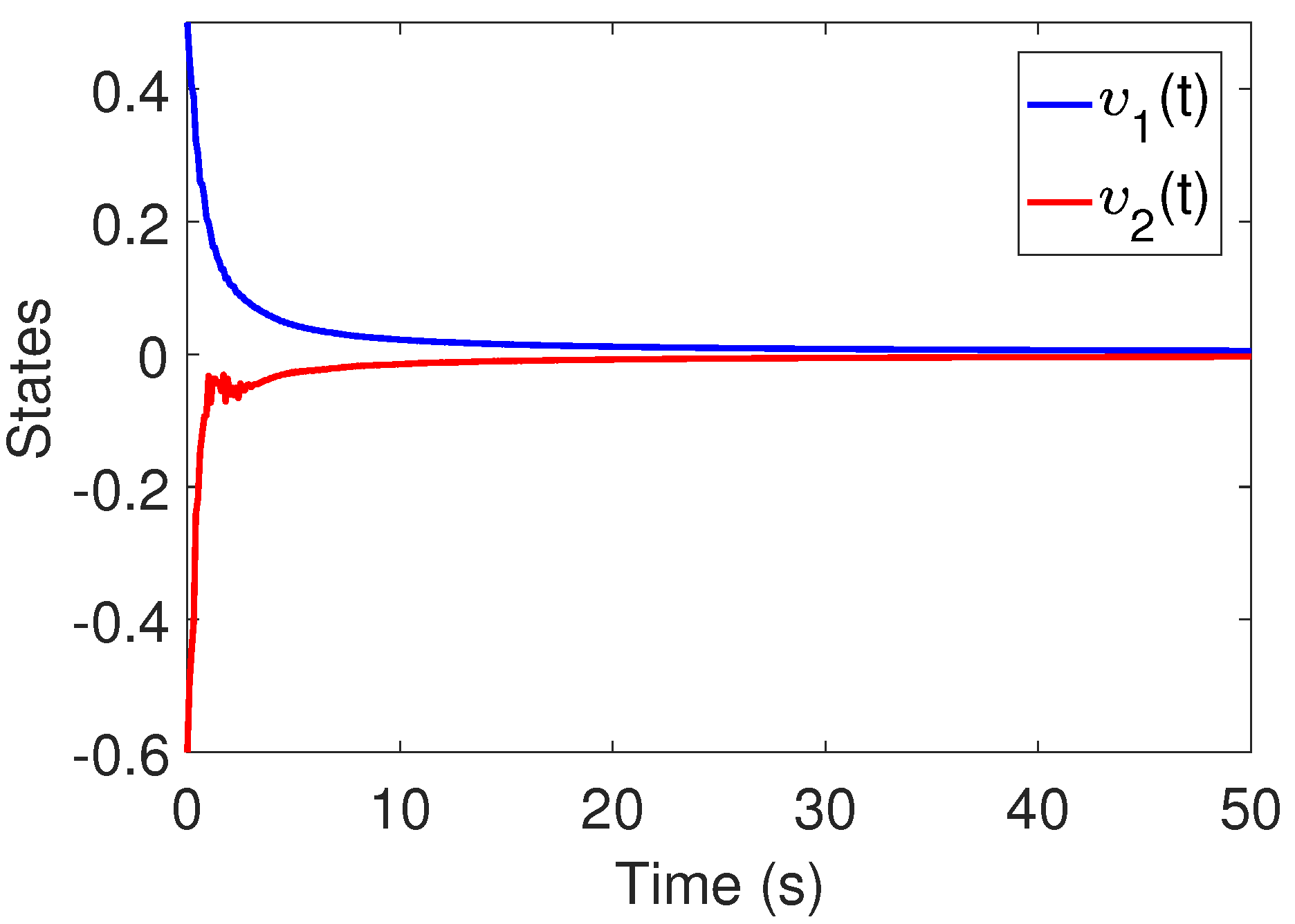
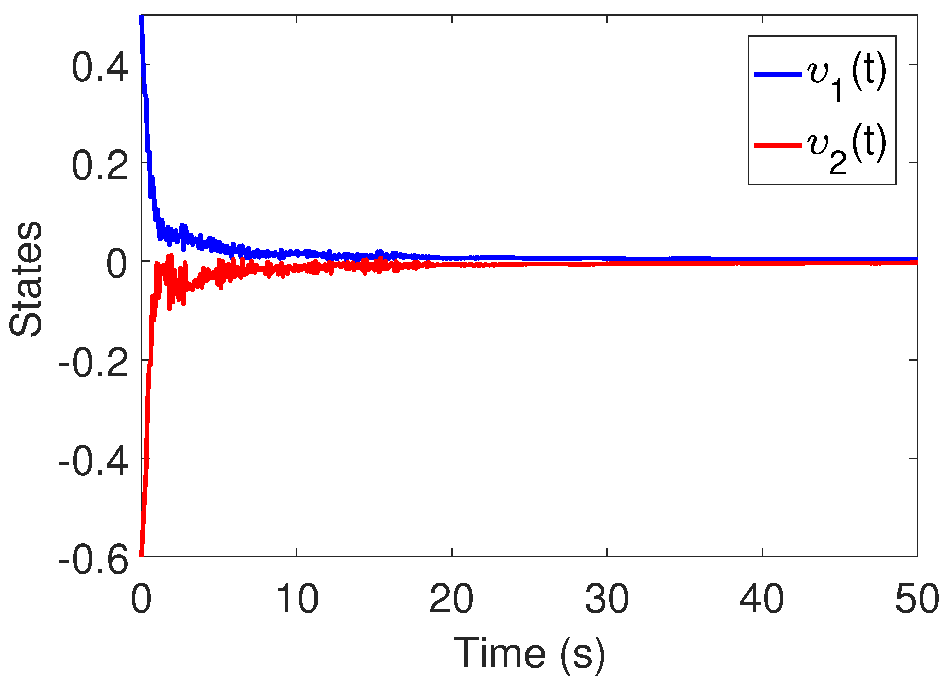
6. Simulation Results

We assess the derived approach by means of several numerical examples.

Example 1. 

Consider the FDS (6) with $\varrho =0.8$ and

$$\begin{array}{cc}\hfill \mathcal{A}& =\left(\begin{array}{cc}1& 2.5\\ 0& -0.6\end{array}\right),{\mathcal{A}}_d=\left(\begin{array}{cc}-0.4& 0\\ 0.6& -0.5\end{array}\right),\hfill \\ \hfill {\mathcal{A}}_0& =\left(\begin{array}{cc}0.2& 0\\ 0.1& 0.4\end{array}\right),E=\left(\begin{array}{cc}1& 0\\ 0& 0\end{array}\right),\mathcal{B}=\left(\begin{array}{c}1\\ 1\end{array}\right).\hfill \end{array}$$

Choosing $\mu \left(t\right)=0.4\left|sin\left(t\right)\right|+0.2$, that is, ${\mu }_m=0.6,{\mu }^{★}=0.4$, and letting $Y=\left(\begin{array}{c}0\\ 1\end{array}\right)$, it is obvious that $\det (s^{\varrho }E-\mathcal{A})=0.6s^{0.8}-0.6,$ is not identically equal to zero. Therefore, the nominal system (6) is regular. Additionally, as $\mathrm{deg}\left[\det (s^{\varrho }E-\mathcal{A})\right]=\mathrm{rank}\left(E\right)=1$, system (6) is impulse-free. However, it is unstable because the root of the polynomial does not satisfy the condition $\left|\arg \right(\mathrm{spec}(E,\mathcal{A})\left)\right|>0.4\pi$. Indeed, the open-loop time response of (6), that is, with $u\left(t\right)=0$, confirms instability, as shown by the states’ trajectories depicted in Figure 3.

Now, a state-feedback control law is designed to ensure the stability of the closed-loop nominal system (6). By solving condition (36) of Theorem 3, we get:

$$\begin{array}{cc}\hfill \mathcal{P}& =\left(\begin{array}{cc}0.9563& 0.0316\\ 0.0316& 1.0909\end{array}\right),\mathcal{Q}=\left(\begin{array}{cc}0.4217& -0.2064\\ -0.2064& 3.4260\end{array}\right),\hfill \\ \hfill \mathcal{Z}& =\left(\begin{array}{cc}0.2584& -0.0499\\ -0.0499& 0.3266\end{array}\right),X=\left(\begin{array}{cc}0.8001& 0.0071\\ -0.7278& 1.1777\end{array}\right),\hfill \\ \hfill N& =\left(\begin{array}{c}-0.1593\\ 3.4046\end{array}\right),\mathcal{J}=\left(\begin{array}{cc}-0.0745& -2.8309\end{array}\right).\hfill \end{array}$$

Afterward, we obtain the state-feedback controller gain as $\mathcal{K}=\left(\begin{array}{cc}-2.2673& -2.3900\end{array}\right)$. The states’ trajectories of the controlled nominal system are shown in Figure 4, revealing that it is asymptotically stable.

Next, we design a proper controller for the system with uncertainty via Theorem 5. Considering ${\mathcal{E}}_0=0.3\mathcal{A},{\mathcal{E}}_1=0.3{\mathcal{A}}_d,{\mathcal{E}}_2=0.3{\mathcal{A}}_0$, $\mathcal{G}\left(t\right)=\left(\begin{array}{cc}sin\left(t\right)& 0\\ 0& cos\left(t\right)\end{array}\right)$ and $\mathcal{H}=\left(\begin{array}{cc}0.5& -0.8\\ 0.5& 0.1\end{array}\right)$, we get

$$\begin{array}{cc}\hfill \mathcal{P}& =\left(\begin{array}{cc}0.7866& 0.0606\\ 0.0606& 1.0052\end{array}\right),\mathcal{Q}=\left(\begin{array}{cc}0.2357& -0.0363\\ -0.0363& 2.6255\end{array}\right),\hfill \\ \hfill \mathcal{Z}& =\left(\begin{array}{cc}0.1712& -0.0281\\ -0.0281& 0.3193\end{array}\right),X=\left(\begin{array}{cc}0.5076& -0.0149\\ -0.6043& 0.9348\end{array}\right),\hfill \\ \hfill N& =\left(\begin{array}{c}0.2388\\ 2.8587\end{array}\right),\mathcal{J}=\left(\begin{array}{cc}-0.0938& -2.5612\end{array}\right),{ϵ}_1=0.6908,{ϵ}_2=0.2095,{ϵ}_3=0.1260,\hfill \end{array}$$

and the gain is $\mathcal{K}=\left(\begin{array}{cc}-3.5134& -2.7959\end{array}\right)$. The states’ trajectories of the controlled uncertain system are shown in Figure 5, confirming the stabilization of the FDS (6) using the static state-feedback technique, albeit the presence of uncertainty. It should be noted that Theorem 3 does not lead to system stability, as shown in Figure 6.

Example 2. 

Consider the FDS (6) with $\varrho =0.9$ and

$$\begin{array}{cc}\hfill \mathcal{A}& =\left(\begin{array}{ccc}1& 1.5& 0\\ 0& -0.5& 0.1\\ 0& 0& 0.2\end{array}\right),{\mathcal{A}}_d=\left(\begin{array}{ccc}-0.5& 0& 0\\ 0.5& -0.5& 0\\ 0.2& 0& 0.1\end{array}\right),\hfill \\ \hfill {\mathcal{A}}_0& =\left(\begin{array}{ccc}0.1& 0& -0.1\\ 0.1& 0& 0.4\\ 0& 0& 0.1\end{array}\right),E=\left(\begin{array}{ccc}1& 0& 0\\ 0& 1& 0\\ 0& 0& 0\end{array}\right),\mathcal{B}=\left(\begin{array}{c}1\\ 1\\ 1\end{array}\right),\hfill \\ \hfill \mathcal{C}& =\left(\begin{array}{ccc}1& 1& 0\end{array}\right).\hfill \end{array}$$

Choosing $\mu \left(t\right)=0.3\left|cos\left(t\right)\right|+0.3$, that is, ${\mu }_m=0.6$ and ${\mu }^{★}=0.3$, and letting $Y={\left(\begin{array}{ccc}0& 0& 1\end{array}\right)}^T$, we verify that $\det (s^{\varrho }E-\mathcal{A})=0.1(s^{0.9}-1)(2s^{0.9}+1)$. Thus, the determinant is not identically equal to zero, and the nominal system (6) is regular. As $\mathrm{deg}\left[\det (s^{\varrho }E-\mathcal{A})\right]=\mathrm{rank}\left(E\right)=2$, the nominal FDS (6) is impulse-free, but it is unstable because the root of the polynomial does not satisfy condition $\left|\arg \left(\mathrm{spe}c(E,\mathcal{A})\right)\right|>0.9{\displaystyle \frac{\pi }{2}}$. The open-loop time response of the nominal system is shown in Figure 7, which confirms instability.

We design an output-feedback controller such that the closed-loop nominal system (6) is asymptotically stable. Solving condition (43) of Theorem 4, we get:

$$\begin{array}{cc}\hfill \mathcal{P}& =\left(\begin{array}{ccc}0.7792& -0.2757& 0.0448\\ -0.2757& 1.0422& -0.0689\\ 0.0448& -0.0689& 0.6723\\ \end{array}\right),\mathcal{Q}=\left(\begin{array}{ccc}0.4438& 0.1091& 0.6309\\ 0.1091& 0.9218& 0.5282\\ 0.6309& 0.5282& 0.2765\end{array}\right),\hfill \\ \hfill \mathcal{Z}& =\left(\begin{array}{ccc}0.4113& -0.4212& -0.0414\\ -0.4212& 0.5063& 0.0929\\ -0.0414& 0.0929& 1.5357\end{array}\right),X=\left(\begin{array}{ccc}0.3333& -0.2789& -0.0432\\ -0.6900& 0.9560& 0.0303\\ 0.0547& 0.4523& 1.5885\end{array}\right),\hfill \\ \hfill N& =\left(\begin{array}{c}0.8336\\ 0.8241\\ 1.8569\end{array}\right),\mathcal{W}=\left(\begin{array}{ccc}0.0047& -1.0490& -0.8398\end{array}\right),\hfill \end{array}$$

and we determine the asymptotically stabilizing output-feedback gain as $\mathcal{L}=-2.9720$. The system states’ trajectories of the controlled nominal system are shown in Figure 8, revealing stability.

Next, an appropriate controller for the system with uncertainty through Theorem 6. Considering ${\mathcal{E}}_0=0.3\mathcal{A},{\mathcal{E}}_1=0.3{\mathcal{A}}_d,{\mathcal{E}}_2=0.3{\mathcal{A}}_0$, $\mathcal{H}=\left(\begin{array}{ccc}0.5& -0.8& 0.1\\ 0.5& 0.1& 1\\ 0& 0& 0.1\end{array}\right)$, and $\mathcal{G}\left(t\right)=\left(\begin{array}{ccc}sin\left(t\right)& 0& 0\\ 0& cos\left(t\right)& 0\\ 0& 0& cos\left(t\right)\end{array}\right),$ we obtain

$$\begin{array}{cc}\hfill \mathcal{P}& =\left(\begin{array}{ccc}0.6658& -0.1156& 0.0238\\ -0.1156& 0.8006& 0.0107\\ 0.0238& 0.0107& 0.7228\end{array}\right),\mathcal{Q}=\left(\begin{array}{ccc}0.4652& 0.2002& 0.6642\\ 0.2002& 0.8678& 0.5938\\ 0.6642& 0.5938& 0.3300\end{array}\right),\hfill \\ \hfill \mathcal{Z}& =\left(\begin{array}{ccc}0.3825& -0.3838& -0.0096\\ -0.3838& 0.4583& 0.1084\\ -0.0096& 0.1084& 1.7465\end{array}\right),X=\left(\begin{array}{ccc}0.2498& -0.2166& -0.0671\\ -0.4824& 0.7563& 0.2011\\ 0.1600& 0.6099& 1.7672\end{array}\right),\hfill \\ \hfill N& =\left(\begin{array}{c}1.0061\\ 1.0186\\ 1.9525\end{array}\right),\mathcal{W}=\left(\begin{array}{ccc}-0.1535& -1.0218& -1.1564\end{array}\right),{ϵ}_1=0.0030,{ϵ}_2=0.0591,{ϵ}_3=0.0286,\hfill \end{array}$$

and we obtain the controller gain as $\mathcal{L}=-3.2568$. The states’ trajectories of the controlled uncertain system are shown in Figure 9. We verify that the system can be stabilized by the output-feedback controller (9) in about 10 s, and that the system is robustly stable, despite uncertainty. Additionally, it should be noted that Theorem 4 cannot lead to system stability, as illustrated by the states’ trajectories depicted in Figure 10.

7. Conclusions

This paper addressed the robust stability and stabilization of uncertain FDSs with time-varying neutral-type delay. Applying the L-K functional method, sufficient criteria were provided in terms of LMIs to ensure stability, regularity and impulse-free properties. State- and output-feedback controllers were designed for achieving robust stabilization of the closed-loop FDSs under all permissible uncertainties. Simulations verifying the applicability of the proposed approach were presented. The theoretical findings constitute a relevant framework to deal with FDSs, which are crucial in many areas of sciences, engineering and mathematics.

References

1. Dai, L. Singular Control Systems; Springer: Berlin/Heidelberg, Germany, 1989. [Google Scholar]
2. Xu, S.; Lam, J. Robust Control and Filtering of Singular Systems; Springer: Berlin/Heidelberg, Germany, 2006; Volume 332. [Google Scholar]
3. Di, Y.; Zhang, J.X.; Zhang, X. Alternate admissibility LMI criteria for descriptor fractional order systems with 0 < α < 2. Fractal Fract. 2023, 7, 577. [Google Scholar]
4. Yang, H.; Si, X.; Ivanov, I.G. Constrained State Regulation Problem of Descriptor Fractional-Order Linear Continuous-Time Systems. Fractal Fract. 2024, 8, 255. [Google Scholar] [CrossRef]
5. Lewis, F.L. A survey of linear singular systems. Circuits Syst. Signal Process. 1986, 5, 3–36. [Google Scholar] [CrossRef]
6. Feng, Y.; Yagoubi, M. Robust Control of Linear Descriptor Systems; Springer: Berlin/Heidelberg, Germany, 2017. [Google Scholar]
7. Kaczorek, T.; Borawski, K. Descriptor Systems of Integer and Fractional Orders; Springer: Berlin/Heidelberg, Germany, 2021; Volume 367. [Google Scholar]
8. Zhuang, G.; Ma, Q.; Zhang, B.; Xu, S.; Xia, J. Admissibility and stabilization of stochastic singular Markovian jump systems with time delays. Syst. Control. Lett. 2018, 114, 1–10. [Google Scholar] [CrossRef]
9. Wang, H.; Xue, A.; Lu, R. Absolute stability criteria for a class of nonlinear singular systems with time delay. Nonlinear Anal. Theory Methods Appl. 2009, 70, 621–630. [Google Scholar] [CrossRef]
10. Long, S.; Zhong, S. Improved results for stochastic stabilization of a class of discrete-time singular Markovian jump systems with time-varying delay. Nonlinear Anal. Hybrid Syst. 2017, 23, 11–26. [Google Scholar] [CrossRef]
11. Liu, G. New results on stability analysis of singular time-delay systems. Int. J. Syst. Sci. 2017, 48, 1395–1403. [Google Scholar] [CrossRef]
12. Aghayan, Z.S.; Alfi, A.; Machado, J.T. Delay-dependent robust stability analysis of uncertain fractional-order neutral systems with distributed delays and nonlinear perturbations subject to input saturation. Int. J. Nonlinear Sci. Numer. Simul. 2023, 24, 329–347. [Google Scholar] [CrossRef]
13. Salamon, D. Control and Observation of Neutral Systems; Number 91; Pitman Advanced Publishing Program: Boston, MA, USA, 1984. [Google Scholar]
14. Han, Q.L. Stability analysis for a partial element equivalent circuit (PEEC) model of neutral type. Int. J. Circuit Theory Appl. 2005, 33, 321–332. [Google Scholar] [CrossRef]
15. Cui, K.; Lu, J.; Li, C.; He, Z.; Chu, Y.M. Almost sure synchronization criteria of neutral-type neural networks with Lévy noise and sampled-data loss via event-triggered control. Neurocomputing 2019, 325, 113–120. [Google Scholar] [CrossRef]
16. Kuang, Y. Delay Differential Equations: With Applications in Population Dynamics; Academic Press: Cambridge, MA, USA, 1993. [Google Scholar]
17. Chen, W.; Zhuang, G.; Xu, S.; Liu, G.; Li, Y.; Zhang, Z. New results on stabilization for neutral type descriptor hybrid systems with time-varying delays. Nonlinear Anal. Hybrid Syst. 2022, 45, 101172. [Google Scholar] [CrossRef]
18. Chen, W.b.; Gao, F. New results on stability analysis for a kind of neutral singular systems with mixed delays. Eur. J. Control 2020, 53, 59–67. [Google Scholar] [CrossRef]
19. Wang, J.; Zhang, Q.; Xiao, D.; Bai, F. Robust stability analysis and stabilisation of uncertain neutral singular systems. Int. J. Syst. Sci. 2016, 47, 3762–3771. [Google Scholar] [CrossRef]
20. Guo, Y.; Li, T. Fractional-order modeling and optimal control of a new online game addiction model based on real data. Commun. Nonlinear Sci. Numer. Simul. 2023, 121, 107221. [Google Scholar] [CrossRef]
21. Chen, Y.; Lv, Z. A fractional optimal control model for a simple cash balance problem. Commun. Nonlinear Sci. Numer. Simul. 2023, 120, 107194. [Google Scholar] [CrossRef]
22. Ortigueira, M.D.; Machado, J.T. The 21st century systems: An updated vision of continuous-time fractional models. IEEE Circuits Syst. Mag. 2022, 22, 36–56. [Google Scholar] [CrossRef]
23. Abdoon, M.A.; Saadeh, R.; Berir, M.; Guma, F.E.; ali, M. Analysis, modeling and simulation of a fractional-order influenza model. Alex. Eng. J. 2023, 74, 231–240. [Google Scholar] [CrossRef]
24. Yunus, A.O.; Olayiwola, M.O.; Omoloye, M.A.; Oladapo, A.O. A fractional order model of lassa disease using the Laplace-adomian decomposition method. Healthc. Anal. 2023, 3, 100167. [Google Scholar] [CrossRef]
25. Mok, R.; Ahmad, M.A. Smoothed functional algorithm with norm-limited update vector for identification of continuous-time fractional-order Hammerstein models. IETE J. Res. 2024, 70, 1814–1832. [Google Scholar] [CrossRef]
26. Baleanu, D.; Sadat Sajjadi, S.; Jajarmi, A.; Asad, J.H. New features of the fractional Euler-Lagrange equations for a physical system within non-singular derivative operator. Eur. Phys. J. Plus 2019, 134, 1–10. [Google Scholar] [CrossRef]
27. Valério, D.; Ortigueira, M.D.; Lopes, A.M. How many fractional derivatives are there? Mathematics 2022, 10, 737. [Google Scholar] [CrossRef]
28. Yakoub, Z.; Aoun, M.; Amairi, M.; Chetoui, M. Identification of continuous-time fractional models from noisy input and output signals. In Fractional Order Systems—Control Theory and Applications: Fundamentals and Applications; Springer: Cham, Switzerland, 2022; pp. 181–216. [Google Scholar]
29. Ortigueira, M.D.; Ionescu, C.M.; Machado, J.T.; Trujillo, J.J. Fractional signal processing and applications. Signal Process. 2015, 107, 197. [Google Scholar] [CrossRef]
30. Ostalczyk, P. Discrete Fractional Calculus: Applications in Control and Image Processing; World Scientific: Singapore, 2015; Volume 4. [Google Scholar]
31. Safaei, M.; Tavakoli, S. Smith predictor based fractional-order control design for time-delay integer-order systems. Int. J. Dyn. Control 2018, 6, 179–187. [Google Scholar] [CrossRef]
32. Modiri, A.; Mobayen, S. Adaptive terminal sliding mode control scheme for synchronization of fractional-order uncertain chaotic systems. ISA Trans. 2020, 105, 33–50. [Google Scholar] [CrossRef]
33. Baishya, C.; Premakumari, R.; Samei, M.E.; Naik, M.K. Chaos control of fractional order nonlinear Bloch equation by utilizing sliding mode controller. Chaos Solitons Fractals 2023, 174, 113773. [Google Scholar] [CrossRef]
34. Caponetto, R. Fractional Order Systems: Modeling and Control Applications; World Scientific: Singapore, 2010; Volume 72. [Google Scholar]
35. Monje, C.A.; Chen, Y.; Vinagre, B.M.; Xue, D.; Feliu-Batlle, V. Fractional-Order Systems and Controls: Fundamentals and Applications; Springer Science & Business Media: Berlin, Germany, 2010. [Google Scholar]
36. Wei, Y.; Zhao, L.; Wei, Y.; Cao, J. Lyapunov theorem for stability analysis of nonlinear nabla fractional order systems. Commun. Nonlinear Sci. Numer. Simul. 2023, 126, 107443. [Google Scholar] [CrossRef]
37. Čermák, J.; Kisela, T. Stabilization and destabilization of fractional oscillators via a delayed feedback control. Commun. Nonlinear Sci. Numer. Simul. 2023, 117, 106960. [Google Scholar] [CrossRef]
38. Jia, J.; Huang, X.; Li, Y.; Cao, J.; Alsaedi, A. Global stabilization of fractional-order memristor-based neural networks with time delay. IEEE Trans. Neural Netw. Learn. Syst. 2019, 31, 997–1009. [Google Scholar] [CrossRef] [PubMed]
39. Hei, X.; Wu, R. Finite-time stability of impulsive fractional-order systems with time-delay. Appl. Math. Model. 2016, 40, 4285–4290. [Google Scholar] [CrossRef]
40. Yu, R.; Wang, D. Structural properties and poles assignability of LTI singular systems under output feedback. Automatica 2003, 39, 685–692. [Google Scholar] [CrossRef]
41. Chen, W.H.; Zheng, W.X.; Lu, X. Impulsive stabilization of a class of singular systems with time-delays. Automatica 2017, 83, 28–36. [Google Scholar] [CrossRef]
42. Sadati, M.; Hosseinzadeh, M.; Shafiee, M. Modelling and analysis of quadruped walking robot using singular system theory. In Proceedings of the 2013 21st Iranian Conference on Electrical Engineering (ICEE), Mashhad, Iran, 14–16 May 2013; pp. 1–6. [Google Scholar]
43. Luenberger, D.G.; Arbel, A. Singular dynamic Leontief systems. Econom. J. Econom. Soc. 1977, 45, 991–995. [Google Scholar] [CrossRef]
44. Stott, B. Power system dynamic response calculations. Proc. IEEE 1979, 67, 219–241. [Google Scholar] [CrossRef]
45. Sell, G.R. Stability theory and Lyapunov’s second method. Arch. Ration. Mech. Anal. 1963, 14, 108–126. [Google Scholar] [CrossRef]
46. Zhang, H.; Ye, R.; Liu, S.; Cao, J.; Alsaedi, A.; Li, X. LMI-based approach to stability analysis for fractional-order neural networks with discrete and distributed delays. Int. J. Syst. Sci. 2018, 49, 537–545. [Google Scholar] [CrossRef]
47. Chaibi, N.; Tissir, E.H. Delay dependent robust stability of singular systems with time-varying delay. Int. J. Control. Autom. Syst. 2012, 10, 632–638. [Google Scholar] [CrossRef]
48. Long, S.; Wu, Y.; Zhong, S.; Zhang, D. Stability analysis for a class of neutral type singular systems with time-varying delay. Appl. Math. Comput. 2018, 339, 113–131. [Google Scholar] [CrossRef]
49. Li, D.; Wei, L.; Song, T.; Jin, Q. Study on asymptotic stability of fractional singular systems with time delay. Int. J. Control Autom. Syst. 2020, 18, 1002–1011. [Google Scholar] [CrossRef]
50. Liu, X.; Wang, P.; Anderson, D.R. On stability and feedback control of discrete fractional order singular systems with multiple time-varying delays. Chaos Solitons Fractals 2022, 155, 111740. [Google Scholar] [CrossRef]
51. Mathiyalagan, K.; Balachandran, K. Finite-time stability of fractional-order stochastic singular systems with time delay and white noise. Complexity 2016, 21, 370–379. [Google Scholar] [CrossRef]
52. Qiu, H.; Wang, H.; Pan, Y.; Cao, J.; Liu, H. Stability and L-Gain of Positive Fractional-Order Singular Systems with Time-Varying Delays. IEEE Trans. Circuits Syst. II Express Briefs 2023, 70, 3534–3538. [Google Scholar] [CrossRef]
53. Podlubny, I. Fractional Differential Equations: An Introduction to Fractional Derivatives, Fractional Differential Equations, to Methods of Their Solution and Some of Their Applications; Elsevier: Amsterdam, The Netherlands, 1998. [Google Scholar]
54. Zhang, F. The Schur Complement and Its Applications; Springer Science & Business Media: Berlin, Germany, 2006; Volume 4. [Google Scholar]
55. Liu, S.; Jiang, W.; Li, X.; Zhou, X.F. Lyapunov stability analysis of fractional nonlinear systems. Appl. Math. Lett. 2016, 51, 13–19. [Google Scholar] [CrossRef]
56. Zhang, X.; Xiao, M.; Jiang, P. Robust H dynamic output feedback control of linear time-varying periodic fractional order singular systems. In Proceedings of the 2018 Chinese Control And Decision Conference (CCDC), Shenyang, China, 9–11 June 2018; pp. 3066–3071. [Google Scholar]
57. Aghayan, Z.S.; Alfi, A.; Machado, J.T. Robust stability of uncertain fractional order systems of neutral type with distributed delays and control input saturation. ISA Trans. 2021, 111, 144–155. [Google Scholar] [CrossRef] [PubMed]
58. Zhang, X.; Chen, Y. Admissibility and robust stabilization of continuous linear singular fractional order systems with the fractional order α: The 0 < α <1 case. ISA Trans. 2018, 82, 42–50. [Google Scholar] [PubMed]
Figure 1. Control block diagram for the state-feedback controller.
Fractalfract 08 00481 g001
Figure 2. Control block diagram for the output-feedback controller.
Fractalfract 08 00481 g002
Figure 3. States’ trajectories of the nominal FDS (6) of Example 1 without controller.
Fractalfract 08 00481 g003
Figure 4. States’ trajectories of the nominal FDS (6) of Example 1 with the state-feedback controller designed using Theorem 3.
Fractalfract 08 00481 g004
Figure 5. States’ trajectories of the uncertain system (6) of Example 1 with the state-feedback controller designed using Theorem 5.
Fractalfract 08 00481 g005
Figure 6. States’ trajectories of the uncertain system (6) of Example 1 with the state-feedback controller designed using Theorem 3.
Fractalfract 08 00481 g006
Figure 7. States’ trajectories of the nominal FDS (6) of Example 2 without controller.
Fractalfract 08 00481 g007
Figure 8. States’ trajectories of the nominal system (6) of Example 2 with the output-feedback controller designed using Theorem 4.
Fractalfract 08 00481 g008
Figure 9. States’ trajectories of the uncertain system (6) of Example 2 with the output-feedback controller designed using Theorem 6.
Fractalfract 08 00481 g009
Figure 10. States’ trajectories of the uncertain system (6) of Example 2 with the output-feedback controller designed using Theorem 4.
Fractalfract 08 00481 g010
Disclaimer/Publisher’s Note: The statements, opinions and data contained in all publications are solely those of the individual author(s) and contributor(s) and not of MDPI and/or the editor(s). MDPI and/or the editor(s) disclaim responsibility for any injury to people or property resulting from any ideas, methods, instructions or products referred to in the content.