On Martínez–Kaabar Fractal–Fractional Volterra Integral Equations of the Second Kind

Abstract

The extension of the theory of generalized fractal–fractional calculus, named in this article as Martínez–Kaabar Fractal–Fractional (MKFF) calculus, is addressed to the field of integral equations. Based on the classic Adomian decomposition method, by incorporating the MKFF $\alpha ,\gamma$-integral operator, we establish the so-called extended Adomian decomposition method (EADM). The convergence of this proposed technique is also discussed. Finally, some interesting Volterra Integral equations of non-integer order which possess a fractal effect are solved via our proposed approach. The results in this work provide a novel approach that can be employed in solving various problems in science and engineering, which can overcome the challenges of solving various equations, formulated via other classical fractional operators.

1. Introduction

The field of integral equations plays an increasingly essential role in modeling various problems in science and engineering. From the theoretical point of view, various proposed techniques have been developed to obtain different types of integral equations’ solution. Specifically, for a very important case of integral equations, the so-called first and second order Volterra integral equations, have been solved using Taylor series and Laplace transformation [1,2,3,4]. Furthermore, the method of Adomian decomposition constitutes effectively a powerful and easy-to-use semi-analytical technique for solving various types of differential and integral equations [5,6]. This technique indicates a fast convergence of solution [7,8,9].

Fractional calculus constitutes an extension of mathematical analysis that has been the focus of many researchers, both from the point of view of the development of its theory, and for its successful application in the resolution of important problems of the different disciplines of science and technology. Theoretically, the definition of the fractional derivative consists of two formulations: one depends on non-local approximation such as the Riemann–Liouville (RL) and Caputo (Cp) derivatives, and the other one depends on a local conception where such definitions are constructed via incremental ratios such as conformable derivative [10] These definitions’ properties and some of their most important applications in different contexts, such as fractional integral equations, can be consulted in [11,12,13,14,15].

In the last decade, due to the fact that non-local fractional definitions come with various challenges to address, new generalized local formulations have been proposed. However, in [16], the conformable derivative has been criticized in comparison with the Caputo definition for certain functions. To overcome that issue, a new generalized derivative of non-integer order, known as the Abu-Shady–Kaabar derivative (ASKD), has been proposed in [17] to efficiently solve various fractional differential equations without the need for complex numerical techniques, and the obtained results are the same of the results obtained using known fractional derivatives such as RL and Cp. Furthermore, an extension of the theory of ASKD to classical analysis such as special functions and the fixed-point theorem has been discussed in [18,19].

In addition, another local formulation, known as the fractal derivative (FD), has been formulated in [20] with the help of fractal definition, and it has been employed in applications such as turbulence and quantum mechanics [20,21].

A hybrid differentiation approach has been developed by Atangana [22] which combines both fractional and fractal differentiations, with various dynamic system properties that have been indicated such as fractal geometry, memory effect, elastic viscosity, and heterogeneity.

Recently, a new generalized fractal–fractional derivative of a local type, named in this research as the Martínez–Kaabar fractal–fractional (MKFF) derivative, has been proposed [23]. This definition, when applied to some elementary functions, produces results that agree with the corresponding results of the fractal–fractional derivative (FFD) in the Cp sense with the power law, introduced in [22]. Also, in [23], the main elements of MKFF calculus are developed, while a notion of integral is established, and its main properties are discussed.

Based on the successful results obtained by applying the MKFF derivative to some interesting ordinary differential equations, formulated via FFD, our research aims to extend the theory of MKFF calculus to the field of integral equations. To achieve this aim, we have structured our study in several steps, detailed below:

(i)

First, we establish the notion of the MKFF Volterra integral equation, focusing on the equations of the second type in Section 2.

(ii)

Furthermore, we extend the classic Adomian Decomposition method in the context of MKFF Volterra integral equations of the second kind and analyze its convergence in Section 3.

(iii)

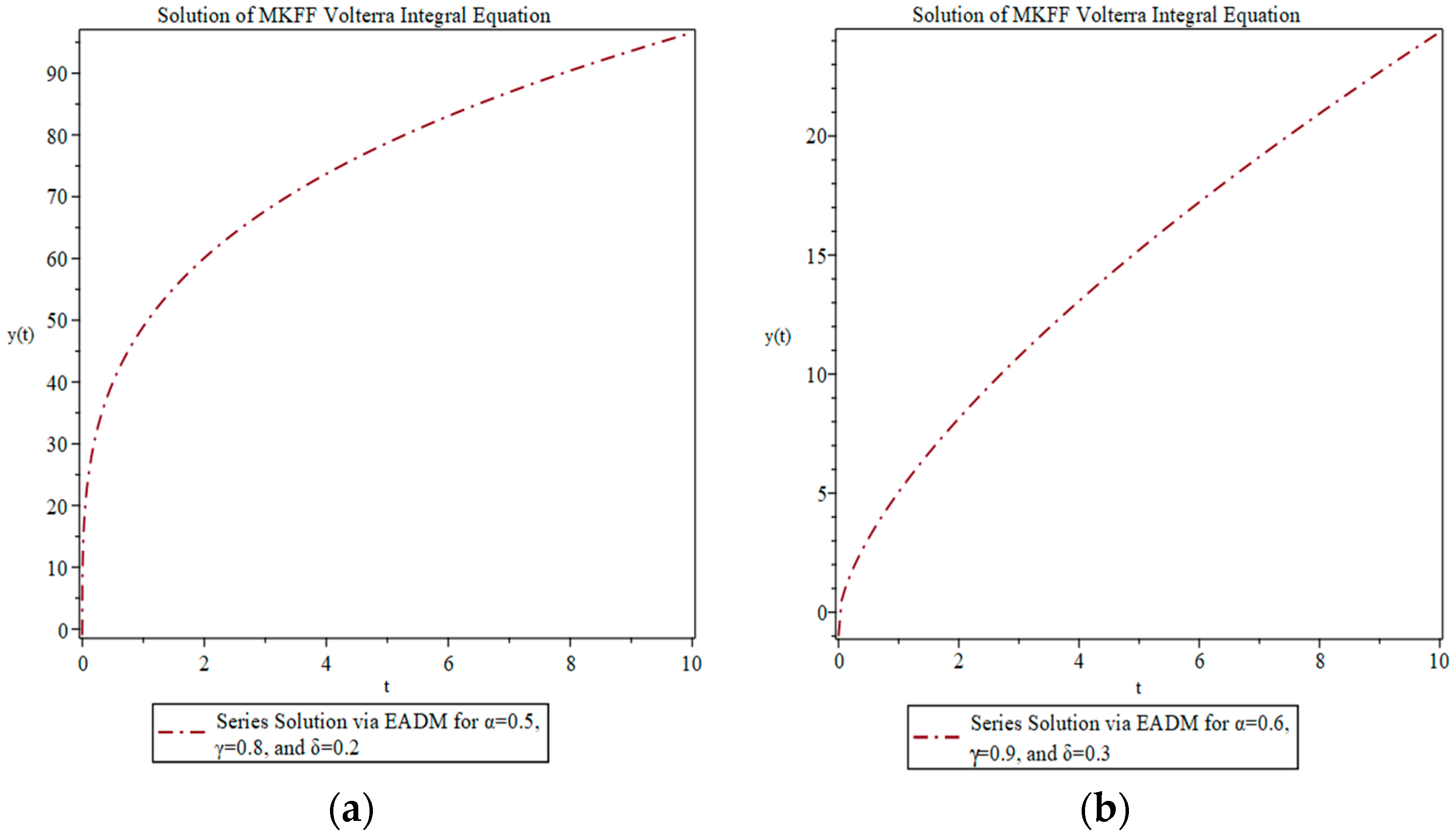
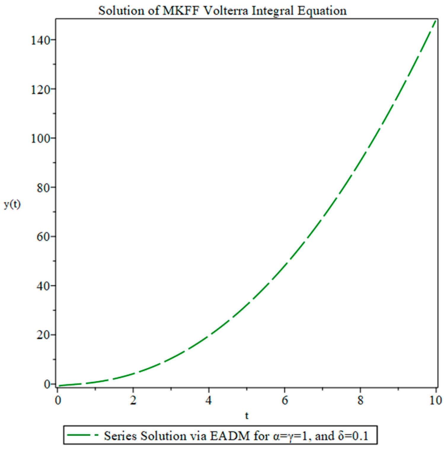
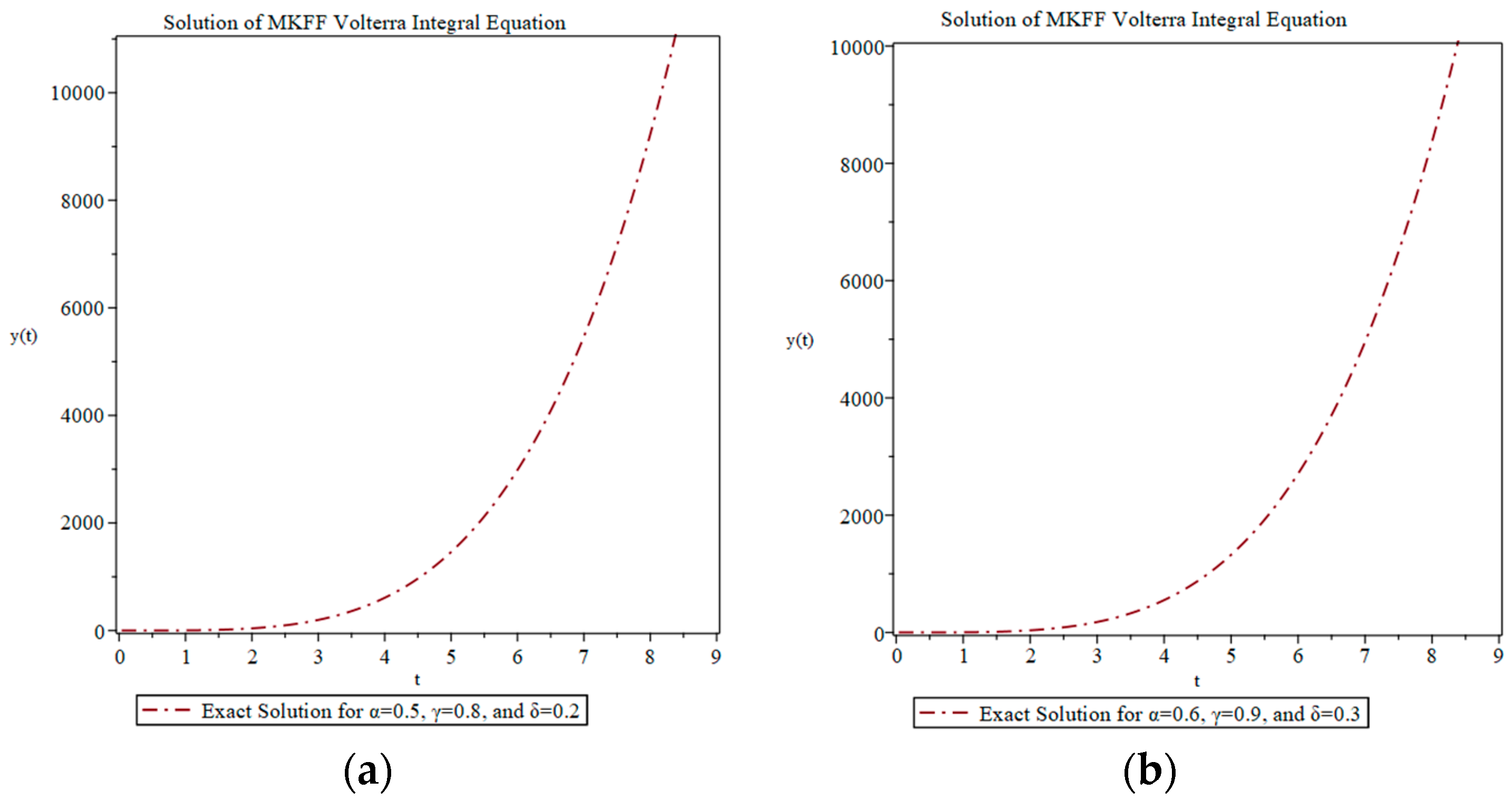
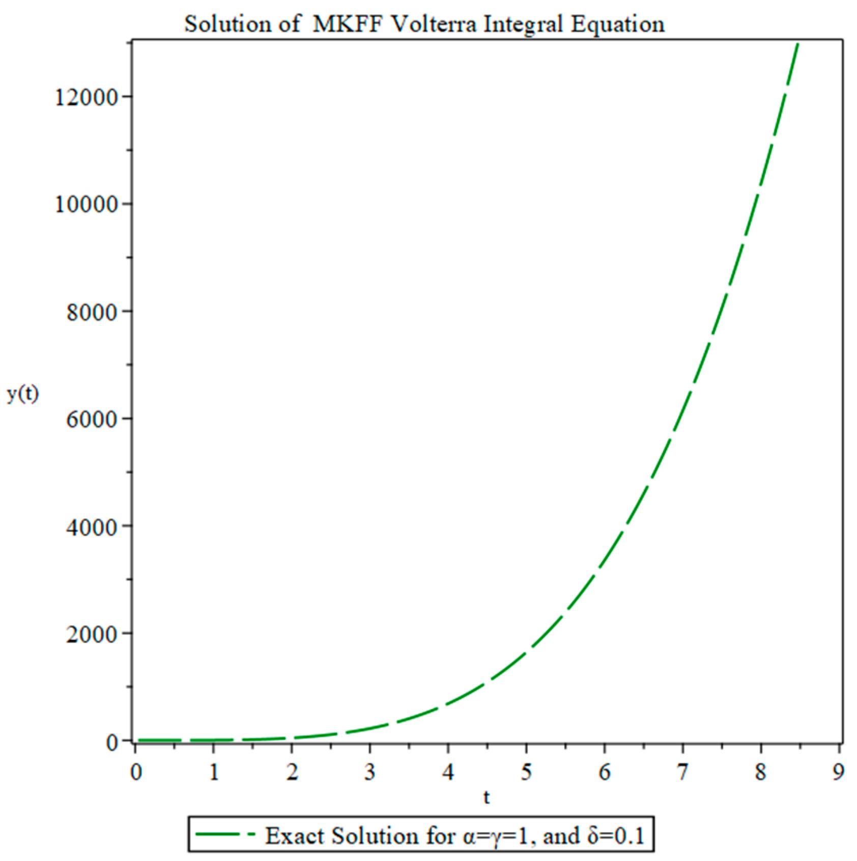
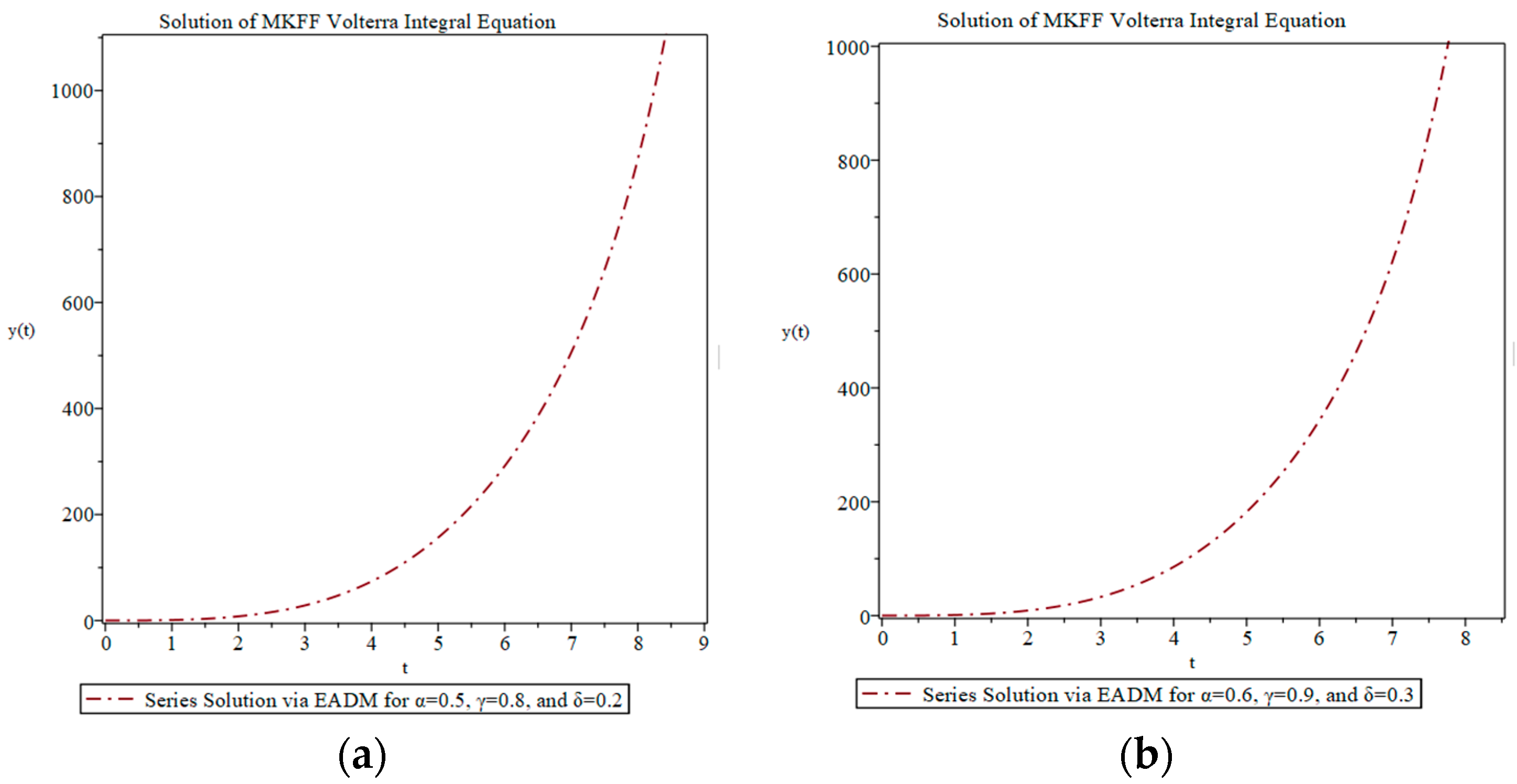
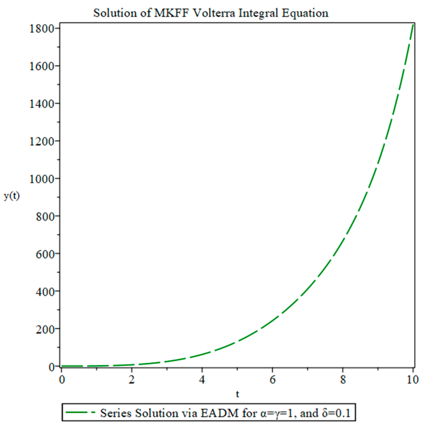
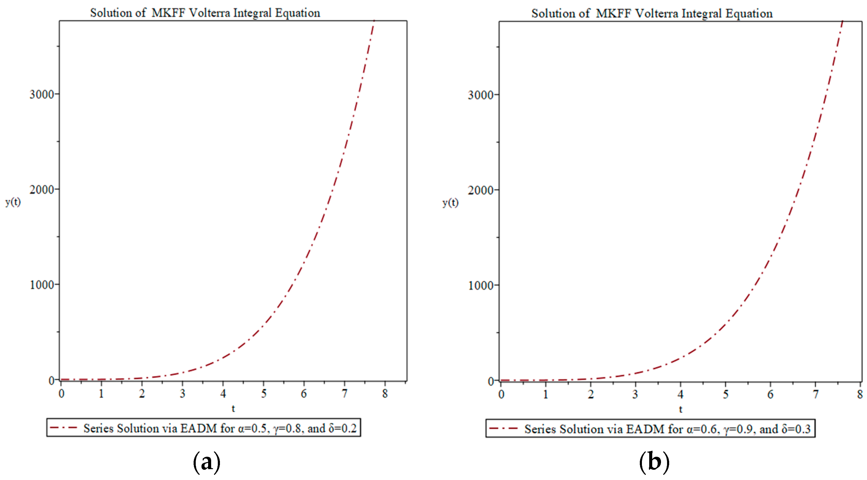
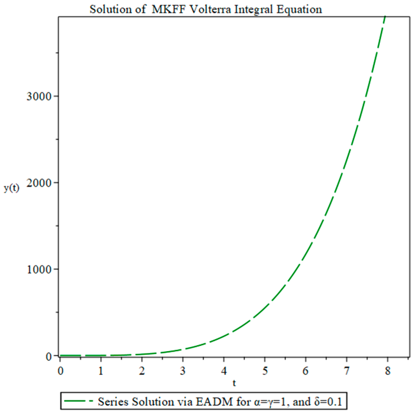
Various applications of the proposed extended Adomian Decomposition Method (EADM) are provided to the MKFF Volterra integral equations of the second kind in Section 4.

(iv)

In Section 5, we conclude our research work with suggested further research extensions and generalizations in future studies. The results in this work are original and unique, and according to the best of our knowledge, our introduced MKFF has never been studied for integral equations before. Therefore, our proposed MKFF with application can effectively help solve various problems in different fields of engineering sciences, mechanics, biology physics, and many others.

2. Preliminaries

Fundamental concepts and results are presented in this section, which are necessary for the developments that we will be presented later. Volterra integral equations, particularly Volterra integral equations formulated via FFD, have been discussed by Araz in [24] from both theoretical and numerical points of view due to their importance in engineering sciences and many other fields. In addition, the integro-differential equations, formulated via FFD, have been recently studied in [25] to form a computational technique to solve such equations via Chelyshkov polynomials. First, the following definition is given from [22] as:

Definition 1. 

$f\left(t\right)$ is assumed to be differentiable on interval $\left[m,\infty )\right.$, with $m\ge 0$, if $f$ is a fractal differentiable on $\left[m,\infty )\right.$ of order $\gamma$, then the FFD of $f$ of order $\alpha$ in Cp sense with power law is expressed as:

$${{}_m{}^{FFD}D}_t^{\alpha ,\gamma }f\left(t\right)={\displaystyle \frac{1}{\mathsf{\Gamma }\left(n-\alpha \right)}}{\int }_m^t{\left(t-\tau \right)}^{n-\alpha -1}{\displaystyle \frac{df\left(\tau \right)}{d{\tau }^{\gamma }}}d\tau , n-1<\alpha ,\gamma \le n, n\in N,$$

(1)

where

$${\displaystyle \frac{df\left(\tau \right)}{d{\tau }^{\gamma }}}=\underset{t\to \tau }{\mathit{lim}}{\displaystyle \frac{f\left(t\right)-f\left(\tau \right)}{t^{\gamma }-{\tau }^{\gamma }}} ,$$

(2)

Remark 1. 

Note that the mentioned ${\displaystyle \frac{df\left(\tau \right)}{d{\tau }^{\gamma }}}$ in Equation (2) is the FD of order $\gamma$, with $\gamma >0$, as proposed in [20,21].

Remark 2. 

Particularly, if we suppose that $m=0$ and $n=1$, then Equation (1) will be reduced as follows:

$${{}_0{}^{FFD}D}_t^{\alpha ,\gamma }f\left(t\right)={\displaystyle \frac{1}{\mathsf{\Gamma }\left(1-\alpha \right)}}{\int }_0^t{\left(t-\tau \right)}^{-\alpha }{\displaystyle \frac{df\left(\tau \right)}{d{\tau }^{\gamma }}}d\tau ,$$

(3)

In relation to the $FFD$ of order α defined in Equation (3), it is also interesting to mention the following two results from [22] as follows:

Theorem 1. 

Assume that $0<\alpha ,\gamma \le 1$, and $\delta >-1$. Then, we obtain:

$${{}_0{}^{FFD}D}_t^{\alpha ,\gamma }(t^{\delta })={\displaystyle \frac{\delta \mathsf{\Gamma }\left(\delta -\gamma +1\right)}{\gamma \mathsf{\Gamma }\left(\delta -\alpha -\gamma +2\right)}}{t}^{\delta -\alpha -\gamma +1},$$

(4)

Remark 3. 

Note that if $f\left(t\right)=c$ for every real constant $c$, then ${{}_0{}^{FFD}D}_t^{\alpha ,\gamma }\left(c\right)=0$.

Theorem 2. 

Suppose that $0<\alpha ,\gamma \le 1$, a function $f\left(t\right)$ is assumed to be analytic at the origin with McLaurin expansion, expressed as:

$$f\left(t\right)=\sum _{j=0}^{\infty }{a}_j{t}^j,$$

(5)

by for $t\in \left[0,k)\right.$ with $k\in R^{+}$. Then, we get:

$${{}_0{}^{FFD}D}_t^{\alpha ,\gamma }f\left(t\right)=\sum _{j=0}^{\infty }{a}_j{{}_0{}^{FFD}D}_t^{\alpha ,\gamma }\left(t^j\right),$$

(6)

Remark 4. 

From Theorem 1, Equation (6) can be written as:

$${{}_0{}^{FFD}D}_t^{\alpha ,\gamma }f\left(t\right)=\sum _{j=1}^{\infty }{a}_j{\displaystyle \frac{j\mathsf{\Gamma }\left(j-\gamma +1\right)}{\gamma \mathsf{\Gamma }\left(j-\alpha -\gamma +2\right)}}{t}^{j-\alpha -\gamma +1},$$

(7)

With the help of Definition 1, Theorems 1 and 2, a new generalized definition of FFD was proposed in [23], and named in this paper as MKFF derivative of order α. The MKFF derivative is defined as follows:

Definition 2. 

A given function: $f:\left[0,\infty \right.)\to R$, the MKFF of order $0<\alpha \le 1$, of $f$ at $t>0$ is expressed as:

$${}^{MKFF}{D}^{\alpha ,\gamma }f\left(t\right)=\underset{\sigma \to 0}{lim}{\displaystyle \frac{f\left(t+\sigma M\left(\alpha ,\gamma ,\delta \right)t^{2-\alpha -\gamma }\right)-f\left(t\right)}{\sigma }},$$

(8)

where $M\left(\alpha ,\gamma ,\delta \right)={\displaystyle \frac{\mathsf{\Gamma }\left(\delta -\gamma +1\right)}{\gamma \mathsf{\Gamma }\left(\delta -\alpha -\gamma +2\right)}}$ with $0<\gamma \le 1$ and $\delta >-1.$

If $f$ is MKFF $\alpha ,\gamma$-differentiable in some $\left(0,m\right)$, $m>0$, and $\underset{t\to 0^{+}}{lim}{}^{MKFF }{D}^{\alpha ,\gamma }f\left(t\right)$ exists, then it is expressed as:

$${}^{MKFF}{D}^{\alpha ,\gamma }f\left(0\right)=\underset{t\to 0^{+}}{\lim }{}^{MKFF}{D}^{\alpha ,\gamma }f\left(t\right),$$

(9)

Remark 5. 

Note that if $\alpha =\gamma =1$, then Equation (8) becomes the classical definition of derivative.

Theorem 3. 

Assume that $0<\alpha ,\gamma \le 1,$ and $f$ is assumed to be a MKFF $\alpha ,\gamma$-differentiable at a point $t>0$. If, additionally, $f$ is differentiable function, then

$${}^{MKFF}{D}^{\alpha ,\gamma }f\left(t\right)={M\left(\alpha ,\gamma ,\delta \right)t}^{2-\alpha -\gamma }{\displaystyle \frac{df(t)}{dt}},$$

(10)

where $M\left(\alpha ,\gamma ,\delta \right)={\displaystyle \frac{\mathsf{\Gamma }\left(\delta -\gamma +1\right)}{\gamma \mathsf{\Gamma }\left(\delta -\alpha -\gamma +2\right)}}$ with $\delta >-1$.

It is interesting to note that as shown in [23], the results, obtained by employing MKFF derivative, are compatible with the results of the FFD of order α in the Cp context with a power law according to Equation (1).

From Definition 2, the following result [23] can be easily shown:

Theorem 4. 

Assume that $0<\alpha ,\gamma \le 1,$ $\delta >-1$ and let $f,h$ be MKFF $\alpha ,\gamma$-differentiable at a point $t>0$. Then, we obtain:

(i) 

${}^{MKFF}{D}^{\alpha ,\gamma }\left(af+bh\right)(t)=a{}^{MKFF}{D}^{\alpha ,\gamma }f(t)+b{}^{MKFF}{D}^{\alpha ,\gamma }h(t)$, $\forall a,b\in R$.

(ii) 

${}^{MKFF}{D}^{\alpha ,\gamma }\left(\varphi \right)=0,$ $\forall$ constant functions $f\left(t\right)=\varphi$.

(iii) 

${}^{MKFF}{D}^{\alpha ,\gamma }\left(fh\right)(t)=f\left(t\right){}^{MKFF}{D}^{\alpha ,\gamma }h(t)+h\left(t\right){}^{MKFF}{D}^{\alpha ,\gamma }f(t)$.

(iv) 

${}^{MKFF}{D}^{\alpha ,\gamma }\left({\displaystyle \frac{f}{h}}\right)(t)={\displaystyle \frac{h\left(t\right){}^{MKFF}{D}^{\alpha ,\gamma }f(t)-f\left(t\right){}^{MKFF}{D}^{\alpha ,\gamma }h(t)}{{[h(t)]}^2}}$.

Given the locality of the MKFF derivative, it is possible to establish a fundamental result of mathematical analysis, the chain rule, in the context of the MKFF calculus [23].

Theorem 5 

(Chain Rule). Suppose that $0<\alpha ,\gamma \le 1,$ $\delta >-1$, $h$ is an MKFF $\alpha ,\gamma$-differentiable at $t>0$ and $f$ is differentiable at $h\left(t\right)$, then

$${}^{MKFF}{D}^{\alpha ,\gamma }\left(f ⃘h\right)\left(t\right)=f^{\prime }\left(h\left(t\right)\right){}^{MKFF}{D}^{\alpha ,\gamma }h\left(t\right).$$

(11)

Remark 6. 

From Theorem 5, the MKFF derivative of order $\alpha$ of the following elementary functions can be easily obtained as follows:

(i) 

${}^{MKFF}{D}^{\alpha ,\gamma }\left({\displaystyle \frac{\gamma }{\left(\alpha +\gamma -1\right)\mathsf{\Gamma }\left(\alpha \right)}}{t}^{\alpha +\gamma -1}\right)=1.$

(ii) 

${}^{MKFF}{D}^{\alpha ,\gamma }\left(e^{{\displaystyle \frac{\gamma }{\left(\alpha +\gamma -1\right)\mathsf{\Gamma }\left(\alpha \right)}}{t}^{\alpha +\gamma -1}}\right)=e^{{\displaystyle \frac{\gamma }{\left(\alpha +\gamma -1\right)\mathsf{\Gamma }\left(\alpha \right)}}{t}^{\alpha +\gamma -1}}.$

(iii) 

${}^{MKFF}{D}^{\alpha ,\gamma }\left(\mathrm{s}\mathrm{i}\mathrm{n}\left({\displaystyle \frac{\gamma }{\left(\alpha +\gamma -1\right)\mathsf{\Gamma }\left(\alpha \right)}}{t}^{\alpha +\gamma -1}\right)\right)=\mathrm{c}\mathrm{o}\mathrm{s}\left({\displaystyle \frac{\gamma }{\left(\alpha +\gamma -1\right)\mathsf{\Gamma }\left(\alpha \right)}}{t}^{\alpha +\gamma -1}\right).$

(iv) 

${}^{MKFF}{D}^{\alpha ,\gamma }\left(\mathrm{c}\mathrm{o}\mathrm{s}\left({\displaystyle \frac{\gamma }{\left(\alpha +\gamma -1\right)\mathsf{\Gamma }\left(\alpha \right)}}{t}^{\alpha +\gamma -1}\right)\right)=-sin\left({\displaystyle \frac{\gamma }{\left(\alpha +\gamma -1\right)\mathsf{\Gamma }\left(\alpha \right)}}{t}^{\alpha +\gamma -1}\right).$

Remark 7. 

Since differentiability indicated that MKFF $\alpha ,\gamma$-differentiability, and supposing that $h\left(t\right)>0$, Equation (11) can be re-written as:

$$\begin{gathered} {}^{MKFF}{D}^{\alpha ,\gamma } \left(f ⃘h\right)\left(t\right)= \\ {\displaystyle \frac{1}{M\left(\alpha ,\gamma ,\delta \right)}}{h\left(t\right)}^{\alpha +\gamma -2}{}^{MKFF}{D}^{\alpha ,\gamma } f\left(h\left(t\right)\right) {}^{MKFF}{D}^{\alpha ,\gamma }h\left(t\right), \end{gathered}$$

(12)

where $M\left(\alpha ,\gamma ,\delta \right)={\displaystyle \frac{\Gamma \left(\delta -\gamma +1\right)}{\gamma \Gamma \left(\delta -\alpha -\gamma +2\right)}}$ where $\delta >-1.$

The mean value theorems of classical mathematical analysis have been extended in [23] to the context of MKFF differentiable functions which is also addressed here, and some interesting consequences are discussed.

In addition, we recall the definition for the MKFF $\alpha ,\gamma$-integral of a function $f$ starting at $m\ge 0$, as proposed in [23].

Definition 3. 

${}^{MKFF}{I}_{\alpha ,\gamma }^m\left(f\right)(t)={\displaystyle \frac{1}{M\left(\alpha ,\gamma ,\delta \right)}}{\int }_m^t{\displaystyle \frac{f(x)}{x^{2-\alpha -\gamma }}}·dx$, such that this integral is the well-known Riemann improper integral, $M\left(\alpha ,\gamma ,\delta \right)={\displaystyle \frac{\mathsf{\Gamma }\left(\delta -\gamma +1\right)}{\gamma \mathsf{\Gamma }\left(\delta -\alpha -\gamma +2\right)}}, 0<\alpha ,\gamma \le 1$, and $\delta >-1.$

According to Definition 3, two essential results are obtained as follows:

Theorem 6. 

${{}^{MKFF}D}^{\alpha ,\gamma }{}^{MKFF}{I}_{\alpha ,\gamma }^m\left(f\right)\left(t\right)=f(t)$, for $t\ge m$, such that $f$ is any continuous function in the domain of ${}^{MKFF}{I}_{\alpha ,\gamma }^m$.

Theorem 7. 

Assume that $m>0$, $0<\alpha ,\gamma \le 1$, $\delta >-1$, and $f$ be a continuous real-valued function on interval $\left[m,w\right]$. Let $H$ be any real-valued function with the property: ${{}^{MKFF}D}^{\alpha ,\gamma }H\left(t\right)=f\left(t\right)$ for all $t\in \left[m,w\right]$. Then,

$${}^{MKFF}{I}_{\alpha ,\gamma }^m\left(f\right)\left(w\right)=H\left(w\right)-H\left(m\right),$$

(13)

3. Results on MKFF Volterra of the Second Kind

The most general standard form of MKFF Volterra integral equations is expressed as:

$$h\left(t\right)y\left(t\right)=f\left(t\right)+{\displaystyle \frac{\beta }{M\left(\alpha ,\gamma ,\delta \right)}}{\int }_0^{t}K\left(t,\tau \right)y\left(\tau \right){\displaystyle \frac{d\tau }{{\tau }^{2-\alpha -\gamma }}},$$

(14)

where $K\left(t,\tau \right)$ is the integral equation’s kernel, $y\left(t\right)$ is an unknown function, $f\left(t\right)$ is a known function (perturbation function), $\beta$ is nonzero real parameter, $M\left(\alpha ,\gamma ,\delta \right)={\displaystyle \frac{\Gamma \left(\delta -\gamma +1\right)}{\gamma \Gamma \left(\delta -\alpha -\gamma +2\right)}}, 0<\alpha ,\gamma \le 1$, and $\delta >-1$. Note that the fractional integral operator involved in the above equation is the MKFF $\alpha ,\gamma$-integral operator. Likewise, if $\alpha =\gamma =1$ is taken in Equation (14), this becomes the classic Volterra integral equation [1,2,3]. On the other hand, if $h\left(t\right)=1$, then Equation (14) simply becomes

$$y\left(t\right)=f\left(t\right)+{\displaystyle \frac{\beta }{M\left(\alpha ,\gamma ,\delta \right)}}{\int }_0^{t}K\left(t,\tau \right)y\left(\tau \right){\displaystyle \frac{d\tau }{{\tau }^{2-\alpha -\gamma }}},$$

(15)

and this equation can be called the MKFF Volterra integral equation of the second kind¸ whereas if $h\left(t\right)=0$, then Equation (14) becomes

$$f\left(t\right)+{\displaystyle \frac{\beta }{M\left(\alpha ,\gamma ,\delta \right)}}{\int }_0^{t}K\left(t,\tau \right)y\left(\tau \right){\displaystyle \frac{d\tau }{{\tau }^{2-\alpha -\gamma }}}=0,$$

(16)

which can be called the MKFF Volterra integral equation of the first kind.

3.1. The Extended Adomian Decomposition Method

Now, we present a new practical technique for handling MKFF Volterra integral equations of second kind, the so-called extended Adomian decomposition method (EADM). In this technique, we take a parallel approach to the classical method of Adomian decomposition, which is generally employed to solve both linear and nonlinear differential equations, integral equations, and integro-differential equations. Note that in this new method, the integral operator involved is the MKFF $\alpha ,\gamma$-integral operator.

This technique is basically the method of power series, which is like the perturbation technique. Let us show our technique by representing $y\left(t\right)$ in the form of a series as follows:

$$y\left(t\right)=\sum _{n=0}^{\infty }{y}_n\left(t\right),$$

(17)

where $y_0\left(t\right)$ as the outside term of the integral sign such that $y_0\left(t\right)=f\left(t\right)$.

By substituting Equation (17) into Equation (15), we obtain:

$$\sum _{n=0}^{\infty }{y}_n\left(t\right)=f\left(t\right)+{\displaystyle \frac{\beta }{M\left(\alpha ,\gamma ,\delta \right)}}{\int }_0^{t}K\left(t,\tau \right)\left[\sum _{n=0}^{\infty }{y}_n\left(t\right)\right]{\displaystyle \frac{d\tau }{{\tau }^{2-\alpha -\gamma }}},$$

(18)

The components $y_0\left(t\right), y_1\left(t\right),\dots ,y_n\left(t\right),\dots$ of the unknown function $y\left(t\right)$ which can be determined completely recursively if we set the following:

$$\begin{gathered} y_0\left(t\right)=f\left(t\right), \\ {y}_1\left(t\right)={\displaystyle \frac{\beta }{M\left(\alpha ,\gamma ,\delta \right)}}{\int }_0^{t}K\left(t,\tau \right)y_0\left(\tau \right){\displaystyle \frac{d\tau }{{\tau }^{2-\alpha -\gamma }}}, \\ {y}_2\left(t\right)={\displaystyle \frac{\beta }{M\left(\alpha ,\gamma ,\delta \right)}}{\int }_0^{t}K\left(t,\tau \right)y_1\left(\tau \right){\displaystyle \frac{d\tau }{{\tau }^{2-\alpha -\gamma }}}, \\ ⋮ \\ {y}_n\left(t\right)={\displaystyle \frac{\beta }{M\left(\alpha ,\gamma ,\delta \right)}}{\int }_0^{t}K\left(t,\tau \right)y_{n-1}\left(\tau \right){\displaystyle \frac{d\tau }{{\tau }^{2-\alpha -\gamma }}}, \end{gathered}$$

(19)

and so on. The above set of equations can be expressed in a compact recurrence scheme as:

$$\begin{gathered} y_0\left(t\right)=f\left(t\right), \\ {y}_{n+1}\left(t\right)={\displaystyle \frac{\beta }{M\left(\alpha ,\gamma ,\delta \right)}}{\int }_0^{t}K\left(t,\tau \right)y_n\left(\tau \right){\displaystyle \frac{d\tau }{{\tau }^{2-\alpha -\gamma }}},n\ge 0, \end{gathered}$$

(20)

Remark 8. 

It should be noted that when this decomposition method is applied, it may not be possible to integrate the kernel due to its complexity. In that situation, the series is truncated at a given point to approximate the function $y\left(t\right)$.

3.2. Convergence of the Extended Adomian Decomposition Method (EADM)

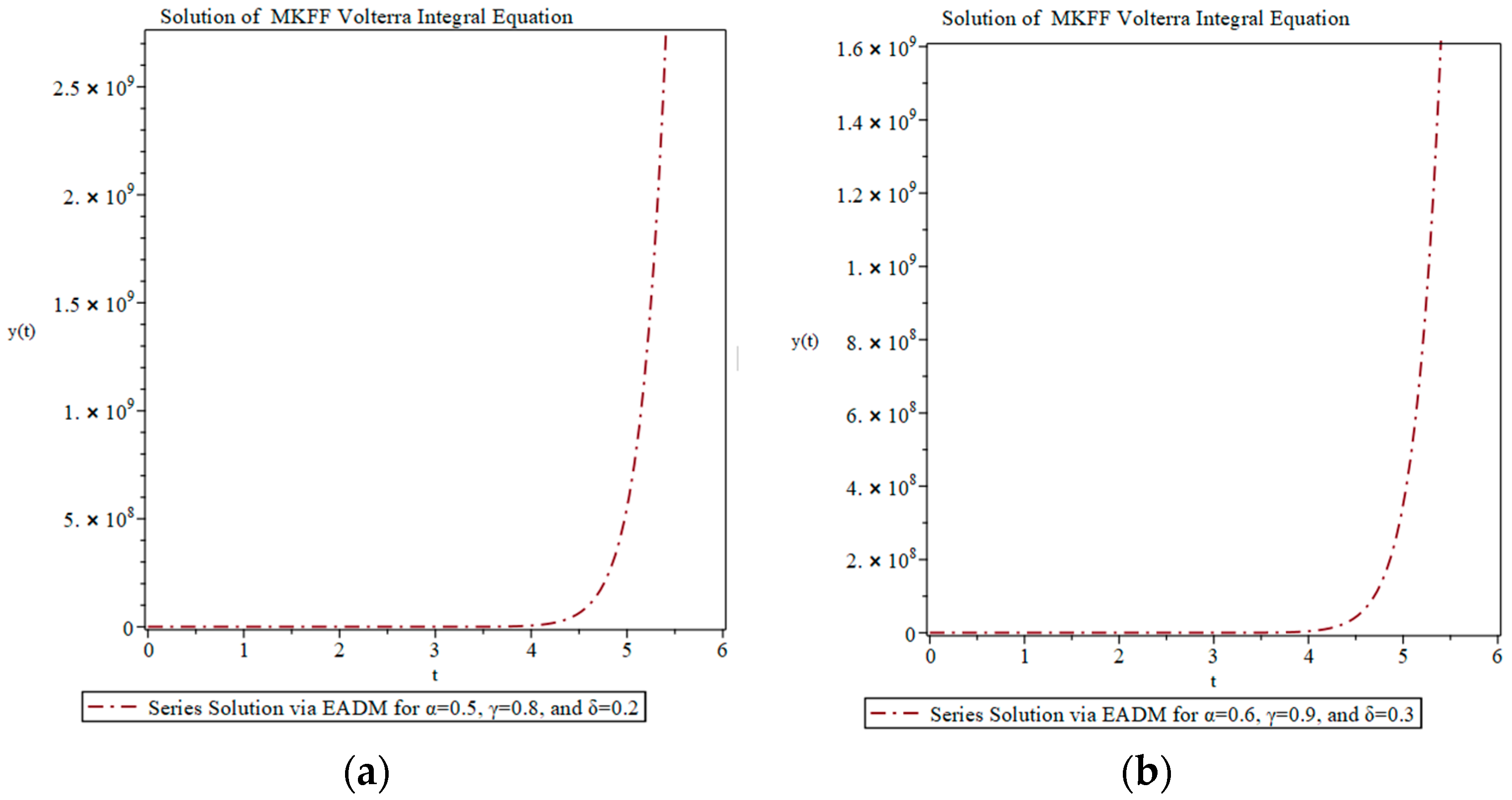
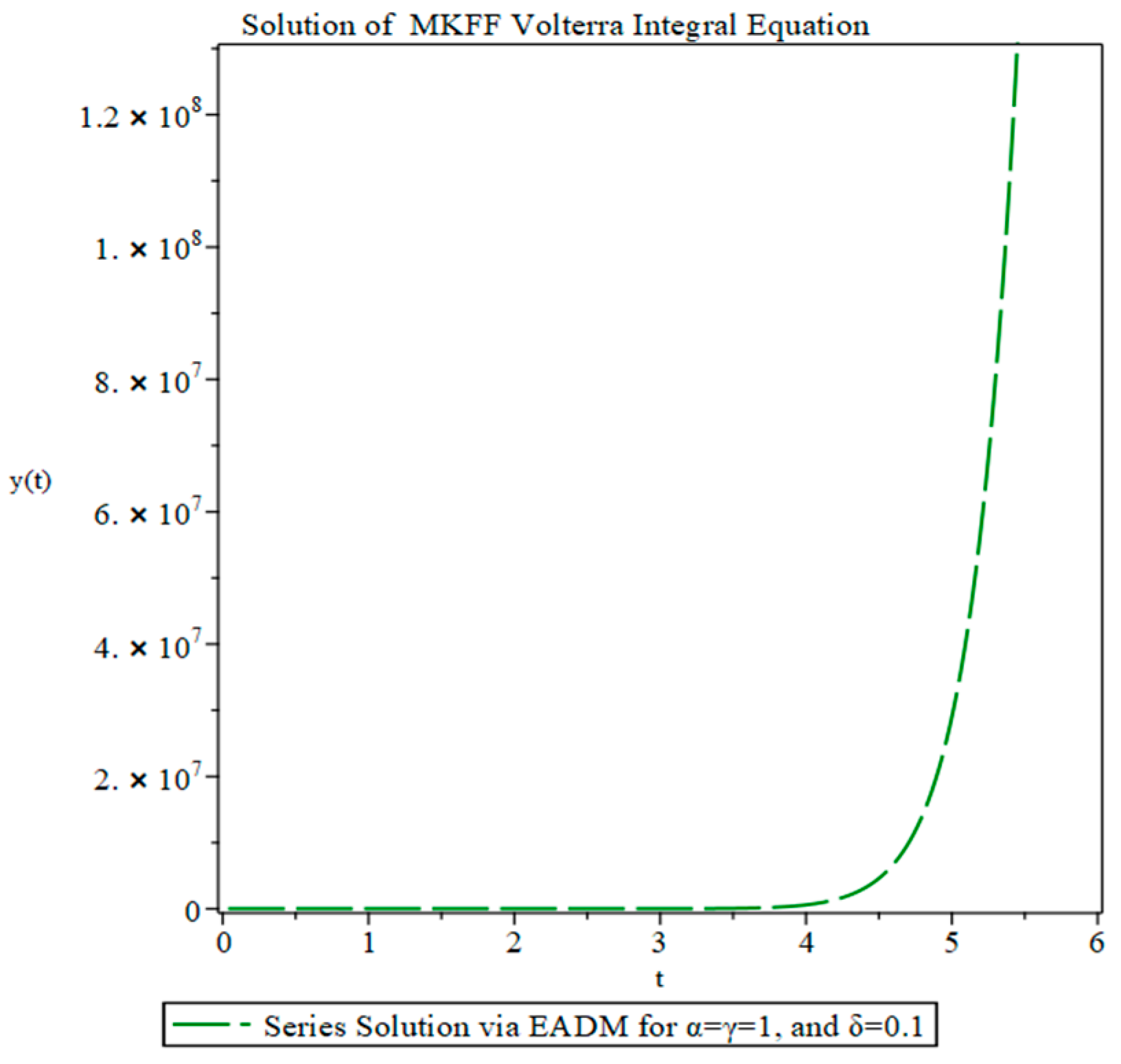
The convergence of the solution of the infinite series is essential to be addressed in this paper. Next, we establish a result in which the convergence of the recurrence scheme in Equation (20) is guaranteed. To prove this result, it is assumed that the parameters $\alpha$ and $\gamma$ involved in the MKFF $\alpha ,\gamma$-integral operator satisfy the following condition: $\alpha +\gamma -1>0, \mathrm{a}\mathrm{n}\mathrm{d} 0<\alpha ,\gamma \le 1$. This requirement ensures the existence of the Riemann improper integrals of the second kind that appear in the developments that we will establish.

Theorem 8. 

If $\left|f\left(t\right)\right|\le P,\forall t\in \left[0,T\right]$ and $\left|K\left(t,\tau \right)\right|\le C,\forall \left(t,\tau \right)\in \left[0,T\right]\times \left[0,T\right]$, then the recurrence scheme in Equation (20) is convergent.

Proof. 

We have the following equalities and inequalities:

$$\begin{gathered} \left|y_0\left(t\right)\right|=\left|f\left(t\right)\right|\le P, \\ \left|y_1\left(t\right)\right|\le {\displaystyle \frac{\left|\beta \right|}{M\left(\alpha ,\gamma , \delta \right)}}\left|{\int }_0^{t}K\left(t,\tau \right)y_0\left(\tau \right){\displaystyle \frac{d\tau }{{\tau }^{2-\alpha -\gamma }}}\right|\le {\displaystyle \frac{PC\left|\beta \right|}{\left(\alpha +\gamma -1\right)M\left(\alpha ,\gamma ,\delta \right)}}{t}^{\alpha +\gamma -1}, \\ \left|y_2\left(t\right)\right|\le {\displaystyle \frac{\left|\beta \right|}{M\left(\alpha ,\gamma ,\delta \right)}}\left|{\int }_0^{t}K\left(t,\tau \right)y_1\left(\tau \right){\displaystyle \frac{d\tau }{{\tau }^{2-\alpha -\gamma }}}\right|\le {\displaystyle \frac{P}{2!}}{\left({\displaystyle \frac{C\left|\beta \right|t^{\alpha +\gamma -1}}{\left(\alpha +\gamma -1\right)M\left(\alpha ,\gamma ,\delta \right)}}\right)}^2, \\ ⋮ \\ \left|y_n\left(t\right)\right|\le {\displaystyle \frac{\left|\beta \right|}{M\left(\alpha ,\gamma ,\delta \right)}}\left|{\int }_0^{t}K\left(t,\tau \right)y_{n-1}\left(\tau \right){\displaystyle \frac{d\tau }{{\tau }^{2-\alpha -\gamma }}}\right|\le {\displaystyle \frac{P}{n!}}{\left({\displaystyle \frac{C\left|\beta \right|t^{\alpha +\gamma -1}}{\left(\alpha +\gamma -1\right)M\left(\alpha ,\gamma ,\delta \right)}}\right)}^n, \end{gathered}$$

(21)

Hence from Equation (21), we have:

$$\left|y_n\left(t\right)\right|\le {\displaystyle \frac{P}{n!}}{\left({\displaystyle \frac{C\left|\beta \right|t^{\alpha +\gamma -1}}{\left(\alpha +\gamma -1\right)M\left(\alpha ,\gamma ,\delta \right)}}\right)}^n,n\ge 0,$$

for all $t\in \left[0,T\right]$. By applying the ratio test for fractional power series [26,27], the convergence of the series can be easily shown which is given by:

$$\sum _{n=0}^{\infty }{\displaystyle \frac{P}{n!}}{\left({\displaystyle \frac{C\left|\beta \right|t^{\alpha +\gamma -1}}{\left(\alpha +\gamma -1\right)M\left(\alpha ,\gamma ,\delta \right)}}\right)}^n,$$

for all $t\in \left[0,T\right]$. Therefore, by means of the well-known comparison criterion for series, the convergence of the recurrence scheme in Equation (20) for all $t\in \left[0,T\right]$ is directly followed [28]. □

4. Applications

Interesting MKFF Volterra integral equations of the second kind in the sense of the MKFF $\alpha ,\gamma$-integral operator are solved in this section via the proposed EADM.

Example 1. 

Consider the MKFF Volterra integral equation of the second kind with $f\left(t\right)=-1, \beta =-3^{\alpha +\gamma -1}, K\left(t,\tau \right)=1$

$$y\left(t\right)=-1-{\displaystyle \frac{3^{\alpha +\gamma -1}}{M\left(\alpha ,\gamma ,\delta \right)}}{\int }_0^{t}y\left(\tau \right){\displaystyle \frac{d\tau }{{\tau }^{2-\alpha -\gamma }}},$$

(22)

Assume that $y\left(t\right)={\sum }_{n=0}^{\infty }{y}_n\left(t\right)$ is the solution of Equation (22). Thus, by the substitution into this equation, we get:

$$\sum _{n=0}^{\infty }{y}_n\left(t\right)=-1-{\displaystyle \frac{3^{\alpha +\gamma -1}}{M\left(\alpha ,\gamma ,\delta \right)}}{\int }_0^t\left(\sum _{n=0}^{\infty }{y}_n\left(\tau \right)\right){\displaystyle \frac{d\tau }{{\tau }^{2-\alpha -\gamma }}},$$

Now, by the decomposition of various terms in the following manner, we obtain a set of solutions as follows:

$$\begin{gathered} y_0\left(t\right)=-1, \\ {y}_1\left(t\right)=-{\displaystyle \frac{3^{\alpha +\gamma -1}}{M\left(\alpha ,\gamma ,\delta \right)}}{\int }_0^t{y}_0\left(\tau \right){\displaystyle \frac{d\tau }{{\tau }^{2-\alpha -\gamma }}}={\displaystyle \frac{1}{M\left(\alpha ,\gamma ,\delta \right)\left(\alpha +\gamma -1\right)}}{\left(3t\right)}^{\alpha +\gamma -1}, \\ {y}_2\left(t\right)=-{\displaystyle \frac{3^{\alpha +\gamma -1}}{M\left(\alpha ,\gamma ,\delta \right)}}{\int }_0^t{y}_1\left(\tau \right){\displaystyle \frac{d\tau }{{\tau }^{2-\alpha -\gamma }}}=-{\displaystyle \frac{1}{2!}}{\left({\displaystyle \frac{1}{M\left(\alpha ,\gamma ,\delta \right)\left(\alpha +\gamma -1\right)}}\right)}^2{\left(3t\right)}^{2\left(\alpha +\gamma -1\right)}, \\ {y}_3\left(t\right)=-{\displaystyle \frac{3^{\alpha +\gamma -1}}{M\left(\alpha ,\gamma ,\delta \right)}}{\int }_0^t{y}_2\left(\tau \right){\displaystyle \frac{d\tau }{{\tau }^{2-\alpha -\gamma }}}={\displaystyle \frac{1}{3!}}{\left({\displaystyle \frac{1}{M\left(\alpha ,\gamma ,\delta \right)\left(\alpha +\gamma -1\right)}}\right)}^3{\left(3t\right)}^{3\left(\alpha +\gamma -1\right)}, \\ ⋮ \end{gathered}$$

and so on.

Hence, the solution of the given MKFF Volterra integral equation in a series form is obtained, and the solution is plotted in Figure 1a,b for various values of $\alpha , \gamma , and \delta$ to understand the behavior of solution as follows:

$$\begin{array}{cc}\hfill y\left(t\right)=-1+& {\displaystyle \frac{1}{M\left(\alpha ,\gamma ,\delta \right)\left(\alpha +\gamma -1\right)}}{\left(3t\right)}^{\alpha +\gamma -1}\hfill \\ & \hspace{1em}\hspace{1em}-{\displaystyle \frac{1}{2!}}{\left({\displaystyle \frac{1}{M\left(\alpha ,\gamma ,\delta \right)\left(\alpha +\gamma -1\right)}}\right)}^2{\left(3t\right)}^{2\left(\alpha +\gamma -1\right)}\hfill \\ & \hspace{1em}\hspace{1em}+{\displaystyle \frac{1}{3!}}{\left({\displaystyle \frac{1}{M\left(\alpha ,\gamma ,\delta \right)\left(\alpha +\gamma -1\right)}}\right)}^3{\left(3t\right)}^{3\left(\alpha +\gamma -1\right)}+\dots ,\hfill \end{array}$$

By the fractal–fractional ratio test, where

$$y_n\left(t\right)={\displaystyle \frac{{\left(-1\right)}^{n+1}}{n!}}{\left({\displaystyle \frac{1}{M\left(\alpha ,\gamma ,\delta \right)\left(\alpha +\gamma -1\right)}}\right)}^n{\left(3t\right)}^{n\left(\alpha +\gamma -1\right)}, n\ge 0,$$

it is easily proven that $0\le t<\infty$, which means the series is convergent for all values of $t$ in a finite interval [26,27].

Remark 9. 

Note that if $\alpha =\gamma =1$, then Equation (22) becomes the following classical Volterra integral equation, and the solution is illustrated in Figure 2:

$$y\left(t\right)=-1-3{\int }_0^{t}y\left(\tau \right)d\tau ,$$

which solution is given by:

$$y\left(t\right)=-1+\left(3t\right)-{\displaystyle \frac{{\left(3t\right)}^2}{2!}}+{\displaystyle \frac{{\left(3t\right)}^3}{3!}}-{\displaystyle \frac{{\left(3t\right)}^4}{4!}}+\dots ,$$

That is convergent to the closed-form solution:

$$y\left(t\right)={-e}^{-3t}$$

Example 2. 

Consider the MKFF Volterra integral equation of the second kind with $f\left(t\right)=M\left(\alpha ,\gamma ,\delta \right)t^{5-\alpha -\gamma }-t^{7-\alpha -\gamma }, \beta =7-\alpha -\gamma , K\left(t,\tau \right)={\tau }^{3-\alpha -\gamma }$

$$y\left(t\right)=M\left(\alpha ,\gamma ,\delta \right)t^{5-\alpha -\gamma }-t^{7-\alpha -\gamma }+{\displaystyle \frac{7-\alpha -\gamma }{M\left(\alpha ,\gamma ,\delta \right)}}{\int }_0^t{\tau }^{3-\alpha -\gamma }y\left(\tau \right){\displaystyle \frac{d\tau }{{\tau }^{2-\alpha -\gamma }}},$$

(23)

Suppose that $y\left(t\right)={\sum }_{n=0}^{\infty }{y}_n\left(t\right)$ is the solution of Equation (23). Thus, by substituting into this equation, we obtain:

$$\sum _{n=0}^{\infty }{y}_n\left(t\right)=M\left(\alpha ,\gamma ,\delta \right)t^{5-\alpha -\gamma }-t^{7-\alpha -\gamma }+{\displaystyle \frac{7-\alpha -\gamma }{M\left(\alpha ,\gamma ,\delta \right)}}{\int }_0^t{\tau }^{3-\alpha -\gamma }\left(\sum _{n=0}^{\infty }{y}_n\left(\tau \right)\right){\displaystyle \frac{d\tau }{{\tau }^{2-\alpha -\gamma }}} ,$$

Now, by the decomposition of various terms in the following manner, a set of solutions is obtained as:

$$\begin{gathered} y_0\left(t\right)=M\left(\alpha ,\gamma ,\delta \right)t^{5-\alpha -\gamma }-t^{7-\alpha -\gamma }, \\ {y}_1\left(t\right)={\displaystyle \frac{7-\alpha -\gamma }{M\left(\alpha ,\gamma ,\delta \right)}}{\int }_0^t{\tau }^{3-\alpha -\gamma }{y}_0\left(\tau \right){\displaystyle \frac{d\tau }{{\tau }^{2-\alpha -\gamma }}}=t^{7-\alpha -\gamma }-{\displaystyle \frac{7-\alpha -\gamma }{M\left(\alpha ,\gamma ,\delta \right)}}{\displaystyle \frac{t^{9-\alpha -\gamma }}{9-\alpha -\gamma }} , \\ {y}_2\left(t\right)={\displaystyle \frac{7-\alpha -\gamma }{M\left(\alpha ,\gamma ,\delta \right)}}{\int }_0^t{\tau }^{3-\alpha -\gamma }{y}_1\left(\tau \right){\displaystyle \frac{d\tau }{{\tau }^{2-\alpha -\gamma }}} \\ ={\displaystyle \frac{7-\alpha -\gamma }{M\left(\alpha ,\gamma ,\delta \right)}}{\displaystyle \frac{1}{9-\alpha -\gamma }}{t}^{9-\alpha -\gamma }-{\left({\displaystyle \frac{7-\alpha -\gamma }{M\left(\alpha ,\gamma ,\delta \right)}}\right)}^2{\displaystyle \frac{t^{11-\alpha -\gamma }}{\left(9-\alpha -\gamma \right)\left(11-\alpha -\gamma \right)}} , \\ {y}_3\left(t\right)={\displaystyle \frac{7-\alpha -\gamma }{M\left(\alpha ,\gamma ,\delta \right)}}{\int }_0^t{\tau }^{3-\alpha -\gamma }{y}_2\left(\tau \right){\displaystyle \frac{d\tau }{{\tau }^{2-\alpha -\gamma }}} \\ ={\left({\displaystyle \frac{7-\alpha -\gamma }{M\left(\alpha ,\gamma ,\delta \right)}}\right)}^2{\displaystyle \frac{1}{\left(9-\alpha -\gamma \right)\left(11-\alpha -\gamma \right)}}{t}^{11-\alpha -\gamma }-{\left({\displaystyle \frac{7-\alpha -\gamma }{M\left(\alpha ,\gamma ,\delta \right)}}\right)}^3{\displaystyle \frac{t^{13-\alpha -\gamma }}{\left(9-\alpha -\gamma \right)\left(11-\alpha -\gamma \right)\left(13-\alpha -\gamma \right)}} , \\ ⋮ \end{gathered}$$

and so on.

Thus, the exact solution of the given fractal–fractional Volterra integral equation is obtained by $y\left(t\right)=M\left(\alpha ,\gamma ,\delta \right)t^{5-\alpha -\gamma }$.

The exact solution is plotted in Figure 3a,b for various values of $\alpha , \gamma , and \delta$ to understand the behavior of solution.

Remark 10. 

Note that if $\alpha =\gamma =1$, then Equation (23) becomes the following classical Volterra integral equation:

$$y\left(t\right)=t^3-t^5+5{\int }_0^t\tau y\left(\tau \right)d\tau ,$$

where the exact solution is given by $y\left(t\right)=t^3$, and the solution is illustrated in Figure 4.

Example 3. 

Consider the MKFF Volterra integral equation of the second kind with $f\left(t\right)={\displaystyle \frac{{\left(2t\right)}^{5-2\alpha -2\gamma }}{\left(5-2\alpha -2\gamma \right)M\left(\alpha ,\gamma ,\delta \right)}}, \beta ={\displaystyle \frac{4}{\left(3-\alpha -\gamma \right)M\left(\alpha ,\gamma ,\delta \right)}}, K\left(t,\tau \right)={\tau }^{3-\alpha -\gamma }-t^{3-\alpha -\gamma }$

$$\begin{gathered} y\left(t\right)={\displaystyle \frac{{\left(2t\right)}^{5-2\alpha -2\gamma }}{\left(5-2\alpha -2\gamma \right)M\left(\alpha ,\gamma ,\delta \right)}} \\ +{\displaystyle \frac{4}{\left(3-\alpha -\gamma \right){\left(M\left(\alpha ,\gamma ,\delta \right)\right)}^2}}{\int }_0^t\left({\tau }^{3-\alpha -\gamma }-t^{3-\alpha -\gamma }\right)y\left(\tau \right){\displaystyle \frac{d\tau }{{\tau }^{2-\alpha -\gamma }}} , \end{gathered}$$

(24)

Suppose that $y\left(t\right)={\sum }_{n=0}^{\infty }{y}_n\left(t\right)$ is Equation (24)’s solution. Thus, by the substitution into this equation, we get:

$$\begin{gathered} \sum _{n=0}^{\infty }{y}_n\left(t\right)={\displaystyle \frac{{\left(2t\right)}^{5-2\alpha -2\gamma }}{\left(5-2\alpha -2\gamma \right)M\left(\alpha ,\gamma ,\delta \right)}} \\ +{\displaystyle \frac{4}{\left(3-\alpha -\gamma \right){\left(M\left(\alpha ,\gamma ,\delta \right)\right)}^2}}{\int }_0^t\left({\tau }^{3-\alpha -\gamma }-t^{3-\alpha -\gamma }\right)\left(\sum _{n=0}^{\infty }{y}_n\left(\tau \right)\right){\displaystyle \frac{d\tau }{{\tau }^{2-\alpha -\gamma }}}, \end{gathered}$$

Now, by the decomposition of various terms in the following manner, a set of solutions is obtained as:

$$\begin{gathered} y_0\left(t\right)={\displaystyle \frac{{\left(2t\right)}^{5-2\alpha -2\gamma }}{\left(5-2\alpha -2\gamma \right)M\left(\alpha ,\gamma ,\delta \right)}} , \\ {y}_1\left(t\right)={\displaystyle \frac{4}{\left(3-\alpha -\gamma \right){\left(M\left(\alpha ,\gamma ,\delta \right)\right)}^2}}{\int }_0^t\left({\tau }^{3-\alpha -\gamma }-t^{3-\alpha -\gamma }\right)y_0\left(\tau \right){\displaystyle \frac{d\tau }{{\tau }^{2-\alpha -\gamma }}}=-{\displaystyle \frac{{\left(2t\right)}^{7-2\alpha -2\gamma }}{\left(5-2\alpha -2\gamma \right)\left(4-\alpha -\gamma \right)\left(7-2\alpha -2\gamma \right){\left(M\left(\alpha ,\gamma ,\delta \right)\right)}^3}} , \\ {y}_2\left(t\right)={\displaystyle \frac{4}{\left(3-\alpha -\gamma \right){\left(M\left(\alpha ,\gamma ,\delta \right)\right)}^2}}{\int }_0^t\left({\tau }^{3-\alpha -\gamma }-t^{3-\alpha -\gamma }\right)y_1\left(\tau \right){\displaystyle \frac{d\tau }{{\tau }^{2-\alpha -\gamma }}} \\ ={\displaystyle \frac{{\left(2t\right)}^{9-2\alpha -2\gamma }}{\left(5-2\alpha -2\gamma \right)\left(4-\alpha -\gamma \right)\left(7-2\alpha -2\gamma \right)\left(6-\alpha -\gamma \right)\left(9-2\alpha -2\gamma \right){\left(M\left(\alpha ,\gamma ,\delta \right)\right)}^5}}, \\ {y}_3\left(t\right)={\displaystyle \frac{4}{\left(3-\alpha -\gamma \right){\left(M\left(\alpha ,\gamma ,\delta \right)\right)}^2}}{\int }_0^t\left({\tau }^{3-\alpha -\gamma }-t^{3-\alpha -\gamma }\right)y_2\left(\tau \right){\displaystyle \frac{d\tau }{{\tau }^{2-\alpha -\gamma }}} \\ =-{\displaystyle \frac{{\left(2t\right)}^{11-2\alpha -2\gamma }}{\left(5-2\alpha -2\gamma \right)\left(4-\alpha -\gamma \right)\left(7-2\alpha -2\gamma \right)\left(6-\alpha -\gamma \right)\left(9-2\alpha -2\gamma \right)\left(8-\alpha -\gamma \right)\left(11-2\alpha -2\gamma \right){\left(M\left(\alpha ,\gamma ,\delta \right)\right)}^7}}, \\ ⋮ \end{gathered}$$

and so on.

Hence, the solution of the given fractal–fractional Volterra integral equation in a series form is obtained, and the solution is plotted in Figure 5a,b for various values of $\alpha , \gamma , and \delta$ to understand the behavior of solution as follows:

$$\begin{gathered} y\left(t\right)={\displaystyle \frac{{\left(2t\right)}^{5-2\alpha -2\gamma }}{\left(5-2\alpha -2\gamma \right)M\left(\alpha ,\gamma ,\delta \right)}}-{\displaystyle \frac{{\left(2t\right)}^{7-2\alpha -2\gamma }}{\left(5-2\alpha -2\gamma \right)\left(4-\alpha -\gamma \right)\left(7-2\alpha -2\gamma \right){\left(M\left(\alpha ,\gamma ,\delta \right)\right)}^3}} \\ +{\displaystyle \frac{{\left(2t\right)}^{9-2\alpha -2\gamma }}{\left(5-2\alpha -2\gamma \right)\left(4-\alpha -\gamma \right)\left(7-2\alpha -2\gamma \right)\left(6-\alpha -\gamma \right)\left(9-2\alpha -2\gamma \right){\left(M\left(\alpha ,\gamma ,\delta \right)\right)}^5}} \\ \begin{array}{l}-{\displaystyle \frac{{\left(2t\right)}^{11-2\alpha -2\gamma }}{\left(5-2\alpha -2\gamma \right)\left(4-\alpha -\gamma \right)\left(7-2\alpha -2\gamma \right)\left(6-\alpha -\gamma \right)\left(9-2\alpha -2\gamma \right)\left(8-\alpha -\gamma \right)\left(11-2\alpha -2\gamma \right){\left(M\left(\alpha ,\gamma ,\delta \right)\right)}^7}}\\ \hspace{1em}\hspace{1em}\hspace{1em}\hspace{1em}\hspace{1em}\hspace{1em}+\dots ,\end{array} \end{gathered}$$

By the fractal–fractional ratio test, where

$$y_n\left(t\right)={\displaystyle \frac{{\left(-1\right)}^n{\left(2t\right)}^{2n+5-2\alpha -2\gamma }}{\left(5-2\alpha -2\gamma \right)\left(4-\alpha -\gamma \right)\left(7-2\alpha -2\gamma \right)\dots \left(2n+2-\alpha -\gamma \right)\left(2n+5-2\alpha -2\gamma \right){\left(M\left(\alpha ,\gamma ,\delta \right)\right)}^{2n+1}}} ,$$

for $n\ge 1$, it is easily proven that $0\le t<\infty$, which implies the convergence of series for all values of $t$ in a finite interval [26,27].

Remark 11. 

Note that if $\alpha =\gamma =1$, then Equation (24) becomes the following classical Volterra integral equation:

$$y\left(t\right)=t+4{\int }_0^t\left(\tau -t\right)y\left(\tau \right)d\tau ,$$

and its solution is given by:

$$y\left(t\right)=\left(2t\right)-{\displaystyle \frac{{\left(2t\right)}^3}{3!}}+{\displaystyle \frac{{\left(2t\right)}^5}{5!}}-{\displaystyle \frac{{\left(2t\right)}^7}{7!}}+\dots ,$$

that is convergent to the closed-form solution:

$$y\left(t\right)=\mathrm{s}\mathrm{i}\mathrm{n}\left(2t\right),$$

and the solution is illustrated in Figure 6.

Example 4. 

Consider the MKFF Volterra integral equation of the second kind with $f\left(t\right)=t^{6-2\alpha -2\gamma }, \beta ={\displaystyle \frac{4}{\left(3-\alpha -\gamma \right)M\left(\alpha ,\gamma ,\delta \right)}}, K\left(t,\tau \right)={\tau }^{3-\alpha -\gamma }-t^{3-\alpha -\gamma }$

$$y\left(t\right)=t^{6-2\alpha -2\gamma }+{\displaystyle \frac{1}{\left(3-\alpha -\gamma \right){\left(M\left(\alpha ,\gamma ,\delta \right)\right)}^2}}{\int }_0^t\left({\tau }^{3-\alpha -\gamma }-t^{3-\alpha -\gamma }\right)y\left(\tau \right){\displaystyle \frac{d\tau }{{\tau }^{2-\alpha -\gamma }}},$$

(25)

Assume that $y\left(t\right)={\sum }_{n=0}^{\infty }{y}_n\left(t\right)$ is Equation (25)’s solution. Thus, we substitute into this equation, and we get:

$$\sum _{n=0}^{\infty }{y}_n\left(t\right)=t^{6-2\alpha -2\gamma }+{\displaystyle \frac{4}{\left(3-\alpha -\gamma \right){\left(M\left(\alpha ,\gamma ,\delta \right)\right)}^2}}{\int }_0^t\left({\tau }^{3-\alpha -\gamma }-t^{3-\alpha -\gamma }\right)\left(\sum _{n=0}^{\infty }{y}_n\left(\tau \right)\right){\displaystyle \frac{d\tau }{{\tau }^{2-\alpha -\gamma }}},$$

Now, by the decomposition of various terms in the following manner, we obtain a set of solutions as follows:

$$\begin{gathered} y_0\left(t\right)=t^{6-2\alpha -2\gamma }, \\ {y}_1\left(t\right)={\displaystyle \frac{1}{\left(3-\alpha -\gamma \right){\left(M\left(\alpha ,\gamma ,\delta \right)\right)}^2}}{\int }_0^t\left({\tau }^{3-\alpha -\gamma }-t^{3-\alpha -\gamma }\right)y_0\left(\tau \right){\displaystyle \frac{d\tau }{{\tau }^{2-\alpha -\gamma }}}={\displaystyle \frac{t^{8-2\alpha -2\gamma }}{\left(5-\alpha -\gamma \right)\left(8-2\alpha -2\gamma \right){\left(M\left(\alpha ,\gamma ,\delta \right)\right)}^2}}, \\ {y}_2\left(t\right)={\displaystyle \frac{1}{\left(3-\alpha -\gamma \right){\left(M\left(\alpha ,\gamma ,\delta \right)\right)}^2}}{\int }_0^t\left({\tau }^{3-\alpha -\gamma }-t^{3-\alpha -\gamma }\right)y_1\left(\tau \right){\displaystyle \frac{d\tau }{{\tau }^{2-\alpha -\gamma }}}={\displaystyle \frac{t^{10-2\alpha -2\gamma }}{\left(5-\alpha -\gamma \right)\left(8-2\alpha -2\gamma \right)\left(7-\alpha -\gamma \right)\left(10-2\alpha -2\gamma \right){\left(M\left(\alpha ,\gamma ,\delta \right)\right)}^4}}, \\ {y}_3\left(t\right)={\displaystyle \frac{1}{\left(3-\alpha -\gamma \right){\left(M\left(\alpha ,\gamma ,\delta \right)\right)}^2}}{\int }_0^t\left({\tau }^{3-\alpha -\gamma }-t^{3-\alpha -\gamma }\right)y_2\left(\tau \right){\displaystyle \frac{d\tau }{{\tau }^{2-\alpha -\gamma }}} \\ ={\displaystyle \frac{t^{12-2\alpha -2\gamma }}{\left(5-\alpha -\gamma \right)\left(8-2\alpha -2\gamma \right)\left(7-\alpha -\gamma \right)\left(10-2\alpha -2\gamma \right)\left(9-\alpha -\gamma \right)\left(12-2\alpha -2\gamma \right){\left(M\left(\alpha ,\gamma ,\delta \right)\right)}^6}} , \\ ⋮ \end{gathered}$$

and so on.

Thus, the solution of the given fractal–fractional Volterra integral equation in a series form is obtained, and the solution is plotted in Figure 7a,b for various values of $\alpha , \gamma , and \delta$ to understand the behavior of solution as follows:

$$\begin{gathered} y\left(t\right)=t^{6-2\alpha -2\gamma }+{\displaystyle \frac{t^{8-2\alpha -2\gamma }}{\left(5-\alpha -\gamma \right)\left(8-2\alpha -2\gamma \right){\left(M\left(\alpha ,\gamma ,\delta \right)\right)}^2}} \\ +{\displaystyle \frac{t^{10-2\alpha -2\gamma }}{\left(5-\alpha -\gamma \right)\left(8-2\alpha -2\gamma \right)\left(7-\alpha -\gamma \right)\left(10-2\alpha -2\gamma \right){\left(M\left(\alpha ,\gamma ,\delta \right)\right)}^4}} \\ +{\displaystyle \frac{t^{12-2\alpha -2\gamma }}{\left(5-\alpha -\gamma \right)\left(8-2\alpha -2\gamma \right)\left(7-\alpha -\gamma \right)\left(10-2\alpha -2\gamma \right)\left(9-\alpha -\gamma \right)\left(12-2\alpha -2\gamma \right){\left(M\left(\alpha ,\gamma ,\delta \right)\right)}^6}}+\dots , \end{gathered}$$

By the fractal–fractional ratio test, where

$$y_n\left(t\right)={\displaystyle \frac{t^{2n+6-2\alpha -2\gamma }}{\left(5-\alpha -\gamma \right)\left(8-2\alpha -2\gamma \right)\left(7-\alpha -\gamma \right)\left(10-2\alpha -2\gamma \right)\dots \left(2n+3-\alpha -\gamma \right)\left(2n+6-2\alpha -2\gamma \right){\left(M\left(\alpha ,\gamma ,\delta \right)\right)}^{2n}}} ,$$

for $n\ge 1$, it is easily proven that $0\le t<\infty$ which implies the convergence of series for all values of $t$ in a finite interval [26,27].

Remark 12. 

Note that if $\alpha =\gamma =1$, then Equation (25) becomes the following classical Volterra integral equation:

$$y\left(t\right)=t^2+{\int }_0^t\left(\tau -t\right)y\left(\tau \right)d\tau ,$$

and its solution is given by

$$y\left(t\right)={\displaystyle \frac{t^2}{2!}}+{\displaystyle \frac{t^4}{4!}}+{\displaystyle \frac{t^6}{6!}}+{\displaystyle \frac{t^8}{8!}}+\dots ,$$

that is convergent to the closed-form solution as follows:

$$y\left(t\right)=2cosht-2,$$

and the solution is illustrated in Figure 8.

Example 5. 

Consider the MKFF Volterra integral equation of the second kind with $f\left(t\right)=4-\alpha -\gamma , \beta ={\displaystyle \frac{1}{5-\alpha -\gamma }}, K\left(t,\tau \right)=t^{3-\alpha -\gamma }{\tau }^{7-2\alpha -2\gamma }$

$$y\left(t\right)=4-\alpha -\gamma +{\displaystyle \frac{1}{\left(5-\alpha -\gamma \right)M\left(\alpha ,\gamma ,\delta \right)}}{\int }_0^t{t}^{3-\alpha -\gamma }{\tau }^{7-2\alpha -2\gamma }y\left(\tau \right){\displaystyle \frac{d\tau }{{\tau }^{2-\alpha -\gamma }}},$$

(26)

Assume that $y\left(t\right)={\sum }_{n=0}^{\infty }{y}_n\left(t\right)$ is Equation (26)’s solution. Thus, by substituting into this equation, we get:

$$\sum _{n=0}^{\infty }{y}_n\left(t\right)=4-\alpha -\gamma +{\displaystyle \frac{1}{\left(5-\alpha -\gamma \right)M\left(\alpha ,\gamma ,\delta \right)}}{\int }_0^t{t}^{3-\alpha -\gamma }{\tau }^{7-2\alpha -2\gamma }\left(\sum _{n=0}^{\infty }{y}_n\left(\tau \right)\right){\displaystyle \frac{d\tau }{{\tau }^{2-\alpha -\gamma }}},$$

Now, by the decomposition of various terms in the following manner, we obtain a set of solutions as follows:

$$\begin{gathered} y_0\left(t\right)=4-\alpha -\gamma , \\ {y}_1\left(t\right)={\displaystyle \frac{1}{\left(5-\alpha -\gamma \right)M\left(\alpha ,\gamma ,\delta \right)}}{\int }_0^t{t^{3-\alpha -\gamma }{\tau }^{7-2\alpha -2\gamma }y}_0\left(\tau \right){\displaystyle \frac{d\tau }{{\tau }^{2-\alpha -\gamma }}}={\displaystyle \frac{\left(4-\alpha -\gamma \right)t^{9-2\alpha -2\gamma }}{\left(5-\alpha -\gamma \right)\left(6-\alpha -\gamma \right)M\left(\alpha ,\gamma ,\delta \right)}}, \\ {y}_2\left(t\right)={\displaystyle \frac{1}{\left(5-\alpha -\gamma \right)M\left(\alpha ,\gamma ,\delta \right)}}{\int }_0^t{t}^{3-\alpha -\gamma }{\tau }^{7-2\alpha -2\gamma }{y}_1\left(\tau \right){\displaystyle \frac{d\tau }{{\tau }^{2-\alpha -\gamma }}}={\displaystyle \frac{\left(4-\alpha -\gamma \right)t^{18-4\alpha -4\gamma }}{3{\left(5-\alpha -\gamma \right)}^3\left(6-\alpha -\gamma \right){\left(M\left(\alpha ,\gamma ,\delta \right)\right)}^2}}, \\ {y}_3\left(t\right)={\displaystyle \frac{1}{\left(5-\alpha -\gamma \right)M\left(\alpha ,\gamma ,\delta \right)}}{\int }_0^t{t}^{3-\alpha -\gamma }{\tau }^{7-2\alpha -2\gamma }{y}_2\left(\tau \right){\displaystyle \frac{d\tau }{{\tau }^{2-\alpha -\gamma }}}={\displaystyle \frac{\left(4-\alpha -\gamma \right)t^{27-6\alpha -6\gamma }}{3{\left(5-\alpha -\gamma \right)}^4\left(6-\alpha -\gamma \right)\left(24-5\alpha -5\gamma \right){\left(M\left(\alpha ,\gamma ,\delta \right)\right)}^3}}, \\ ⋮ \end{gathered}$$

and so on.

Hence, the solution of the given fractal–fractional Volterra integral equation in a series form is obtained, and the solution is plotted in Figure 9a,b for various values of $\alpha , \gamma , and \delta$ to understand the behavior of solution as follows:

$$\begin{gathered} y\left(t\right)=4-\alpha -\gamma +{\displaystyle \frac{\left(4-\alpha -\gamma \right)t^{9-2\alpha -2\gamma }}{\left(5-\alpha -\gamma \right)\left(6-\alpha -\gamma \right)M\left(\alpha ,\gamma ,\delta \right)}} \\ +{\displaystyle \frac{\left(4-\alpha -\gamma \right)t^{18-4\alpha -4\gamma }}{3{\left(5-\alpha -\gamma \right)}^3\left(6-\alpha -\gamma \right){\left(M\left(\alpha ,\gamma ,\delta \right)\right)}^2}} \\ +{\displaystyle \frac{\left(4-\alpha -\gamma \right)t^{27-6\alpha -6\gamma }}{3{\left(5-\alpha -\gamma \right)}^4\left(6-\alpha -\gamma \right)\left(24-5\alpha -5\gamma \right){\left(M\left(\alpha ,\gamma ,\delta \right)\right)}^3}}+\dots , \end{gathered}$$

Remark 13. 

Note that if $\alpha =\gamma =1$, then Equation (26) becomes the following classical Volterra integral equation:

$$y\left(t\right)=2+{\displaystyle \frac{1}{3}}{\int }_0^{t}t{\tau }^{3}y\left(\tau \right)d\tau ,$$

where the solution in a series form is given by:

$$y\left(t\right)=2+{\displaystyle \frac{1}{6}}{t}^5+{\displaystyle \frac{1}{6{·3}^3}}{t}^{10}+{\displaystyle \frac{1}{6{·3}^4·14}}{t}^{15}+{\displaystyle \frac{1}{6{·3}^5·14·19}}{t}^{20}+\dots ,$$

and the solution is plotted in Figure 10.

5. Conclusions

In this research article, the extension of the recently introduced MKFF calculus theory has been addressed to the field of fractal–fractional Volterra integral equations. We have focused on the Volterra integral equations of the second kind in the sense of MKFF, for which we have developed an extension of the classic method of Adomian decomposition. This new proposed technique involves the MKFF $\alpha ,\gamma$-integral operator. We also analyzed the convergence of this method based on results from classical and fractional power series. Finally, we have illustrated the application of EADM through various interesting examples. On one hand, the obtained results in this work allow us to conclude that this method, by involving an MKFF $\alpha ,\gamma$-integral operator, provides an efficient mathematical tool to get solutions to several scientific and engineering problems that possess a fractal effect and involve fractional Volterra integral equations of second kind. The graphical representations of all obtained solutions have been provided using MAPLE in this work to illustrate the physical behavior of obtained solutions at various fractional orders and fractal effects. Finally, we have also confirmed that our results represent an extension of the classical theory of Volterra integral equations. The results in this work can be further extended in future studies to work on various differential equations’ types and develop new computational techniques with more real-world applications in physics, engineering, biology, and economics. The complex examples related to Volterra integral equations in [29] can be also studied via MKFF in future studies to provide more insights and contributions about the applicability of MKFF in complex scientific phenomena.

References

1. Rahman, M. Integral Equations and their Applications. Methods and Applications; Wit Press: Boston, MA, USA, 2007. [Google Scholar]
2. Wazwaz, A.M. Linear and Nonlinear Integral Equations. Methods and Applications; Springer: Berlin/Heidelberg, Germany, 2011. [Google Scholar]
3. Wazwaz, A.M. A First Course in Integral Equations, 2nd ed.; World Scientific: Singapore, 2015. [Google Scholar]
4. Aggarwal, S.; Dua, A.; Bhatnagar, K. Method Taylor’s series for the primitive of linear first kind Volterra integral equation. Int. J. Sci. Res. Publ. 2019, 9, 926–931. [Google Scholar]
5. Husain, Y.A.; Bashir, M.A. The Application of Adomian Decomposition Technique to Volterra Integral type of Equation. Int. J. Adv. Res. 2020, 8, 117–120. [Google Scholar] [CrossRef]
6. Emmanuel, F.S. Solution of Integral Equations of Volterra type using the Adomian Decomposition Method (ADM). MathLab J. 2020, 7, 16–23. [Google Scholar]
7. Cherruault, Y.; Saccomandi, G.; Some, B. New results for convergence of Adomian’s Method applied to integral equations. Math. Comput. Model. 1992, 16, 85–93. [Google Scholar] [CrossRef]
8. El-Kalla, I.L. Convergence of the Adomian Method applied to a class of nonlinear integral equations. Appl. Math. Lett. 2008, 21, 372–376. [Google Scholar] [CrossRef]
9. Feng, J.-Q.; Sun, S. Numerical Solution of Volterra Integral Equation by Adomian Decomposition Method. Asian Res. J. Math. 2017, 4, 1–12. [Google Scholar] [CrossRef]
10. Khalil, R.; Al-Horani, M.; Yousef, A.; Sababheh, M. A new definition of fractional derivative. J. Comput. Appl. Math. 2014, 264, 65–70. [Google Scholar] [CrossRef]
11. Miller, K.S. An Introduction to Fractional Calculus and Fractional Differential Equations; J. Wiley & Sons: New York, NY, USA, 1993. [Google Scholar]
12. Podlubny, I. Fractional Differential Equations, Mathematics in Science and Engineering; Academic Press, Inc.: San Diego, CA, USA, 1999. [Google Scholar]
13. Kibas, A.A.; Srivastava, H.M.; Trujillo, J.J. Theory and Applications of Fractional Differential Equations; North-Holland: New York, NY, USA, 2006. [Google Scholar]
14. Arshad, S.; Sun, S.; O’Regan, D. Lp-solutions for fractional integral equations. Fract. Calc. Appl. Anal. 2014, 17, 259–276. [Google Scholar] [CrossRef]
15. Kaewnimit, K.; Wannalookkhee, F.; Orankitjaroen, S. The Solutions of Some Riemann-Liouville Fractional Integral Equations. Fractal Fract. 2021, 5, 154. [Google Scholar] [CrossRef]
16. Abdelhakim, A.A. The flaw in the conformable calculus: It is conformable because it is nor fractional. Fract. Calc. Appl. Anal. 2019, 22, 245–252. [Google Scholar] [CrossRef]
17. Abu-Shady, M.; Kaabar, M.K.A. A Generalized Definition of the Fractional Derivative with Applications. Math. Probl. Eng. 2021, 2021, 9444803. [Google Scholar] [CrossRef]
18. Abu-Shady, M.; Kaabar, M.K.A. A novel computational tool for the fractional-order special functions arising from modelling scientific phenomena via Abu-Shady-Kaabar fractional derivative. Comput. Math. Methods Med. 2022, 2022, 2138775. [Google Scholar] [CrossRef] [PubMed]
19. Martínez, F.; Kaabar, M.K.A. A novel theorical investigation of the Abu-Shady-Kaabar fractional derivative as a modelling tool for science and engineering. Comput. Math. Methods Med. 2022, 2022, 4119082. [Google Scholar] [CrossRef] [PubMed]
20. Chen, W. Time-space fabric underlying anomalous diffusion. Chaos Solitons Fractals 2006, 28, 923–929. [Google Scholar] [CrossRef]
21. Chen, W.; Sun, H.; Zhang, X.; Korosak, D. Anomalous diffusion modeling by fractal and fractional derivatives. Comput. Math. Appl. 2010, 59, 1754–1758. [Google Scholar] [CrossRef]
22. Atangana, A. Fractal-fractional differentiation and integration: Connecting fractal calculus and fractional calculus to predict complex system. Chaos Solitons Fractals 2017, 102, 396–406. [Google Scholar] [CrossRef]
23. Martínez, F.; Kaabar, M.K.A. A new generalized definition of fractal-fractional derivative with some applications. Math. Comput. Appl. 2024, 29, 31. [Google Scholar] [CrossRef]
24. Araz, S.İ. Numerical analysis of a new volterra integro-differential equation involving fractal-fractional operators. Chaos Solitons Fractals 2020, 130, 109396. [Google Scholar] [CrossRef]
25. Rahimkhani, P.; Sedaghat, S.; Ordokhani, Y. An effective computational solver for fractal-fractional 2D integro-differential equations. J. Appl. Math. Comput. 2024, 70, 3411–3440. [Google Scholar] [CrossRef]
26. Al Masalmeh, M. Series Method to solve conformable fractional Riccati differential equations. Int. J. Appl. Math. Res. 2017, 6, 30–33. [Google Scholar] [CrossRef]
27. Martínez, F.; Martínez, I.; Kaabar, M.K.A.; Paredes, S. Some new results on conformable fractional power series. Asia Pac. J. Math. 2020, 7, 1–14. [Google Scholar]
28. Apostol, T.M. Calculus, I, 2nd ed.; John Wiley & Sons: Hoboken, NJ, USA, 1991. [Google Scholar]
29. Providas, E.; Parasidis, I.N. Analytical Solution of n th-Order Volterra Integro-Differential Equations of Convolution Type with Non-local Conditions. In Analysis, Geometry, Nonlinear Optimization and Applications; World Scientific: Singapore, 2023; pp. 659–675. [Google Scholar]
Figure 1. Solution of the given MKFF Volterra integral equation in Example 1: (a) Series solution via EADM for α = 0.5 ,   γ = 0.8 ,   a n d   δ = 0.2 ; (b) series solution via EADM for α = 0.6 ,   γ = 0.9 ,   a n d   δ = 0.3 .
Fractalfract 08 00466 g001
Figure 2. Series solution of the given MKFF Volterra integral equation in Example 1 via EADM for α = γ = 1 ,   a n d   δ = 0.1 .
Fractalfract 08 00466 g002
Figure 3. Exact solution of the given MKFF Volterra integral equation in Example 2: (a) Exact solution for α = 0.5 ,   γ = 0.8 ,   a n d   δ = 0.2 ; (b) exact solution for α = 0.6 ,   γ = 0.9 ,   a n d   δ = 0.3 .
Fractalfract 08 00466 g003
Figure 4. Exact solution of the given MKFF Volterra integral equation in Example 2 via EADM for α = γ = 1 ,   a n d   δ = 0.1 .
Fractalfract 08 00466 g004
Figure 5. Series solution of the given MKFF Volterra integral equation in Example 3: (a) Series solution via EADM for α = 0.5 ,   γ = 0.8 ,   a n d   δ = 0.2 ; (b) series solution via EADM for α = 0.6 ,   γ = 0.9 ,   a n d   δ = 0.3 .
Fractalfract 08 00466 g005
Figure 6. Series solution of the given MKFF Volterra integral equation in Example 3 via EADM for α = γ = 1 ,   a n d   δ = 0.1 .
Fractalfract 08 00466 g006
Figure 7. Series solution of the given MKFF Volterra integral equation in Example 4: (a) Series solution via EADM for α = 0.5 ,   γ = 0.8 ,   a n d   δ = 0.2 ; (b) series solution via EADM for α = 0.6 ,   γ = 0.9 ,   a n d   δ = 0.3 .
Fractalfract 08 00466 g007
Figure 8. Series solution of the given MKFF Volterra integral equation in Example 4 via EADM for α = γ = 1 ,   a n d   δ = 0.1 .
Fractalfract 08 00466 g008
Figure 9. Series solution of the given MKFF Volterra integral equation in Example 5: (a) Series solution via EADM for α = 0.5 ,   γ = 0.8 ,   a n d   δ = 0.2 ; (b) series solution via EADM for α = 0.6 ,   γ = 0.9 ,   a n d   δ = 0.3 .
Fractalfract 08 00466 g009
Figure 10. Series solution of the given MKFF Volterra integral equation in Example 5 via EADM for α = γ = 1 ,   a n d   δ = 0.1 .
Fractalfract 08 00466 g010
Disclaimer/Publisher’s Note: The statements, opinions and data contained in all publications are solely those of the individual author(s) and contributor(s) and not of MDPI and/or the editor(s). MDPI and/or the editor(s) disclaim responsibility for any injury to people or property resulting from any ideas, methods, instructions or products referred to in the content.