Adaptive Synchronization of Fractional-Order Uncertain Complex-Valued Competitive Neural Networks under the Non-Decomposition Method

Abstract

This paper is devoted to the study of adaptive synchronization for fractional-order uncertain complex-valued competitive neural networks (FOUCVCNNs) using the non-decomposition method. Firstly, a new network model named FOUCVCNNs is proposed, which is not separated into two real-valued subsystems in order to keep its intrinsic speciality. In addition, a novel adaptive controller is designed to reduce the cost of control. Meanwhile, with the help of fractional Lyapunov theory, 1-norm analysis framework and inequality techniques, several effective synchronization criteria for FOUCVCNNs are obtained by constructing an appropriate Lyapunov function. Finally, the reliability of the results obtained is tested through numerical simulation.

1. Introduction

With the rapid development of technology, the era of artificial intelligence is coming. As an indispensable component of artificial intelligence, the research on various neural networks (NNs) has attracted widespread attention from many scholars, including but not limited to, Hopfield NNs [1], gene NNs [2], BAM NNs [3], coupled NNs [4], inertial NNs [5] and competitive NNs (CNNs) [6]. Among them, the dynamical analysis of CNNs has received increasing interest from researchers due to its expansive application prospect in numerous fields such as neural computing and pattern recognition. The origin of CNNs can be tracked back to the study of Cohen and Grossberg [7]; since then, a great deal of valuable dynamical results have emerged. For example, Adhira et al. analyzed the exponential dissipative performance of CNNs by proposing two weighted summation inequalities [8]. By designing two new control schemes, Xu et al. obtained mean-square synchronization criteria for CNNs [9]. Based on a novel control framework, the issue of multiple finite-time synchronizations and their settling-time estimation has been addressed by Wang et al. [10].

As one of the most important branches of mathematics, fractional calculus is a matter of great concern owing to its significant application in control sciences and engineering. Taking into consideration their heritability and infinite memory features, fractional-order neural networks (FONNs) have emerged; as such, some interesting research findings have been obtained [11,12,13,14,15]. Recently, some scholars have combined fractional-order derivatives with CNNs to develop fractional-order CNNs (FOCNNs), and derived a lot of successful results related to their passivity [16], stability [16,17,18,19,20,21], and synchronization [21,22,23]. Meanwhile, the impact of uncertain parameters on system modeling and analysis is inevitable, and they may have a negative effect on the dynamical behaviors of NNs. Therefore, it is necessary to consider uncertain parameters in analyzing the dynamics of NNs. Shafiya et al. established uncertain FONNs and investigated their global synchronization by means of improved fractional inequalities [24]. Chen et al. proposed uncertain fractional gene regulatory networks and made some new dynamical achievements [25]. Syed Ali et al. firstly incorporated uncertain parameters into FOCNNs to model uncertain FOCNNs, and dealt with relevant derive–response synchronization issues via the LMI technique [26].

In recent years, the research on complex-valued NNs (CVNNs) has received more and more attention in contrast to real-valued NNs (RVNNs). Since the complexity variable plays an important role in various application areas such as image reconstruction, nonlinear filtering, and pattern classification, CVNNs have more sophisticated characteristics and potential advantages in applications. For instance, the problems of symmetry detection and XOR can be easily resolved by CVNNs, which are difficult to achieve through RVNNs. It is important to note that, if the concept of complex variables is not considered, RVNNs are merely specific circumstances of CVNNs. Accordingly, it is of great significance to explore the dynamics of CVNNs, and many extremely good results have been published in terms of stability analysis [27,28,29] and synchronization control [30,31,32]. As we all know, there are two common research methods for CVNNs, i.e., the separation technique and the non-decomposition method. The former involves splitting CVNNs into two RVNNs, which inevitably leads to an increase in complexity and the redundancy of theory analysis. The latter involves treating CVNNs as a whole to analyze their dynamics directly. However, there is no research on fractional-order uncertain complex-valued CNNs (FOUCVCNNs), let alone the associated findings based on non-decomposition method, which is an interesting problem to be addressed.

Synchronization is a dynamical behavior of the utmost importance, which shows that the coordinated behavior of two or more systems has been finally realized under external control. The study of the synchronization of NNs has grown rapidly due to their widespread application in cryptograph, image processing and so on. It is essential to design effective control strategies to achieve synchronization goals. Currently, some excellent control methods have been developed, such as adaptive control [12,25], quantized control [32], feedback control [33], switching control [34] and pinning control [35]. Significantly, compared with other control strategies, the adaptive method can decrease control costs greatly on account of the self-regulation of control gains. As we have seen, research on the adaptive synchronization of FOUCVCNNs based on the non-decomposition method has not been reported, which is worth exploring further.

Inspired by the above analysis, this paper aims to address the issue of the adaptive synchronization of FOUCVCNNs under the non-decomposition method. The core novelties of this paper are generalized below:

(1)

A novel FOUCVCNNs model is proposed, and its dynamics have been analyzed based on non-decomposition method.

(2)

A new adaptive controller is designed to realize the synchronization of FOUCVCNNs.

(3)

By means of the fractional Lyapunov approach and the inequality technique, some effective synchronization results for FOUCVCNNs have been obtained, which can be further extended to deal with the dynamical study of integer-order one.

The remaining parts of this paper are organized as follows. Section 2 highlights the fractional calculus knowledge and establishes the FOUCVCNNs model. In Section 3, the adaptive synchronization criteria for FOUCVCNNs are derived via the fractional Lyapunov approach. A numerical simulation is then carried out to verify our results in Section 4. Finally, a summarization and the future prospects of this paper are offered in Section 5.

Notation: $\mathbb{R}$, $\mathbb{C}$, ${\mathbb{R}}^{+}$, ${\mathbb{C}}^n$ are the sets of real numbers, complex numbers, positive real numbers and n-dimensional complex space, respectively. For any $p=\mathrm{Re}(p)+i\mathrm{Im}(p)\in \mathbb{C}$, the conjugate of p is represented by $\overline{p}=\mathrm{Re}(p)-i\mathrm{Im}(p)$, ${|p|}_1=|\mathrm{Re}(p)|+|\mathrm{Im}(p)|$, where $\mathrm{Re}(p)$ and $\mathrm{Im}(p)$ denote, respectively, the real part as well as imaginary part of p. For any $P={(p_1,p_2,···,p_n)}^T\in \mathbb{C}$, ${\displaystyle {||P||}_1=\sum _{\iota =1}^n{|p_{\iota }|}_1}$.

2. Model Description and Preliminaries

In this section, some definitions, such as the sign function of the complex variable, the Mittag-Leffler function and fractional calculus, are retrospectively given. In addition, several lemmas, the FOUCVCNNs model and its relevant assumptions are provided.

Definition 1 

([30]). For any complex variable ξ, its sign function is defined by $\left[\xi \right]=\mathrm{sign}\left(\mathrm{Re}(\xi )\right)+i\mathrm{sign}\left(\mathrm{Im}(\xi )\right)$.

Definition 2 

([36]). The Mittag-Leffler function with two parameters can be defined by

$${\mathrm{E}}_{x,y}(\xi )=\sum _{\eta =0}^{\infty }{\displaystyle \frac{{\xi }^{\eta }}{\Gamma (\eta x+y)}},$$

where $x>0$, $y,\xi \in \mathbb{C}$, $\Gamma (·)$ is the Gamma function. In particular, if $y=1$, then it can be reduced to the Mittag-Leffler function with one parameter, i.e., ${\displaystyle {\mathrm{E}}_x(\xi )=\sum _{\eta =0}^{\infty }\frac{{\xi }^{\eta }}{\Gamma (\eta x+1)}}$. Furthermore, the Laplace transform of ${\displaystyle {(t-t_0)}^{y-1}{\mathrm{E}}_{x,y}\left(-\tau {(t-t_0)}^x\right)}$ is given by

$${\displaystyle \mathfrak{L}\left\{{(t-t_0)}^{y-1}{\mathrm{E}}_{x,y}\left(-\tau {(t-t_0)}^x\right)\right\}=\frac{s^{x-y}}{s^x+\tau },}$$

where $\tau \in \mathbb{C}$ and $|\tau s^{-x}|<1$.

Definition 3 

([36]). The Riemann–Liouville fractional integral of $h(t)$ is defined by

$${ }_{t_0}{I}_t^{\gamma }h(t)={\displaystyle \frac{1}{\Gamma (\gamma )}}{\int }_{t_0}^t{(t-l)}^{\gamma -1}h(l)dl,$$

where $\Gamma (\gamma )={\int }_0^{+\infty }{l}^{\gamma -1}{e}^{-l}dl$, $0<\gamma <1$.

Definition 4 

([36]). The Caputo fractional-order derivative within $0<\gamma <1$ is defined as

$${ }_{t_0}^c{D}_t^{\gamma }h(t)={\displaystyle \frac{1}{\Gamma (1-\gamma )}}{\int }_{t_0}^t{\displaystyle \frac{h^{\prime }(l)}{{(t-l)}^{\gamma }}}dl.$$

We consider the following fractional-order uncertain complex-valued competitive neural networks (FOUCVCNNs):

$$\left\{\begin{array}{ccc}{\displaystyle { }_{t_0}^c{D}_t^{\gamma }{\alpha }_{\iota }(t)}& =\hfill & {\displaystyle -a_{\iota }{\alpha }_{\iota }(t)+\sum _{\eta =1}^n\left({\zeta }_{\iota \eta }+▵{\zeta }_{\iota \eta }(t)\right)h_{\eta }({\alpha }_{\eta }(t))+c_{\iota }{\beta }_{\iota }(t)+{\Psi }_{\iota }(t),}\hfill \\ {\displaystyle { }_{t_0}^c{D}_t^{\gamma }{\beta }_{\iota }(t)}& =\hfill & {\displaystyle -\left(b_{\iota }+▵b_{\iota }(t)\right){\beta }_{\iota }(t)+h_{\iota }({\alpha }_{\iota }(t)),}\hfill \end{array}\right.$$

(1)

where $\iota ,\eta \in \mathcal{N}$ in the order of $\gamma \in (0,1)$. ${\alpha }_{\iota }(t)$, ${\beta }_{\iota }(t)$ are the current state of the $\iota$th neuron and the synaptic efficiency, respectively. $a_{\iota }$, $b_{\iota }\in \mathbb{C}$ represent for the neuron self-feedback coefficient, and within them Re$(a_{\iota })$, Re$(b_{\iota })>0$. ${\zeta }_{\iota \eta }$ is the connection weight between neurons. $c_{\iota }$ denotes the external stimulus intensity. $h_{\eta }({\alpha }_{\eta }(t))$ indicates the output activation of $\eta$th neuron. $\Psi (t)$ is the constant external input for $\iota$th neuron. The uncertainty parameters are expressed by $▵{\zeta }_{\iota \eta }(t)$ and $▵b_{\iota }(t)$. In order to facilitate the study, we made the following assumptions.

Assumption 1. 

For any ω, $\varpi \in \mathbb{C}$, there is the positive real number ${\chi }_{\eta }$ such that

$$|h_{\eta }(\varpi )-h_{\eta }(\omega )|\le {\chi }_{\eta }|\varpi -\omega |.$$

Assumption 2. 

For $▵{\zeta }_{\iota \eta }(t)$ and $▵b_{\iota }(t)$, there exist constants ${\zeta }_{\iota \eta }^{★}$ and $b_{\iota }^{★}$ such that $|▵{\zeta }_{\iota \eta }(t)|\le {\zeta }_{\iota \eta }^{★}$, $|▵b_{\iota }(t)|\le b_{\iota }^{★}$.

Remark 1. 

Considering the wide applicability and convenient practicality of the Caputo fractional derivative, accordingly the FOUCVCNNs model we constructed is based on the Caputo form. Currently, some interesting dynamical results have been published, mainly including real-valued competitive neural networks (CNNs) [5,6,7,8,9,10], fractional CNNs [16,17,18,19,20,21,22,23], uncertain CNNs [26] and complex-valued CNNs [29]; our model (1) can be viewed as an extension of the existing ones to some extent.

Regarding FOUCVCNN (1) as the master system, its slave system can be described as follows

$$\left\{\begin{array}{ccc}{\displaystyle { }_{t_0}^c{D}_t^{\gamma }{\widehat{\alpha }}_{\iota }(t)}& =\hfill & {\displaystyle -a_{\iota }{\widehat{\alpha }}_{\iota }(t)+\sum _{\eta =1}^n\left({\zeta }_{\iota \eta }+▵{\zeta }_{\iota \eta }(t)\right)h_{\eta }({\widehat{\alpha }}_{\eta }(t))+c_{\iota }{\widehat{\beta }}_{\iota }(t)+{\Psi }_{\iota }(t)+u_{\iota }^{†}(t),}\hfill \\ {\displaystyle { }_{t_0}^c{D}_t^{\gamma }{\widehat{\beta }}_{\iota }(t)}& =\hfill & {\displaystyle -\left(b_{\iota }+▵b_{\iota }(t)\right){\widehat{\beta }}_{\iota }(t)+h_{\iota }({\widehat{\alpha }}_{\iota }(t))+u_{\iota }^{‡}(t),}\hfill \end{array}\right.$$

(2)

where $u_{\iota }^{†}(t)$ and $u_{\iota }^{‡}(t)$ are the adaptive controllers to be designed as shown below

$$\left\{\begin{array}{ccc}{\displaystyle u_{\iota }^{†}(t)}& =\hfill & {\displaystyle -{\theta }_{\iota }(t)p_{\iota }(t)-\rho \left[p_{\iota }(t)\right],}\hfill \\ {\displaystyle u_{\iota }^{‡}(t)}& =\hfill & {\displaystyle -{\vartheta }_{\iota }(t)q_{\iota }(t)-\varrho \left[q_{\iota }(t)\right],}\hfill \end{array}\right.$$

(3)

where ${ }_{t_0}^c{D}_t^{\gamma }{\theta }_{\iota }(t)={\delta }_{\iota }{|p_{\iota }(t)|}_1$, ${ }_{t_0}^c{D}_t^{\gamma }{\vartheta }_{\iota }(t)={\sigma }_{\iota }{|q_{\iota }(t)|}_1$, ${\delta }_{\iota }$, ${\sigma }_{\iota }$, $\rho$, $\varrho \in {\mathbb{R}}^{+}$.

Based on master system (1) and slave system (2), let $p_{\iota }(t)={\widehat{\alpha }}_{\iota }(t)-{\alpha }_{\iota }(t)$, $q_{\iota }(t)={\widehat{\beta }}_{\iota }(t)-{\beta }_{\iota }(t)$, and then their error system can be easily obtained

$$\left\{\begin{array}{cc}{\displaystyle { }_{t_0}^c{D}_t^{\gamma }{p}_{\iota }(t)=}& {\displaystyle -a_{\iota }{p}_{\iota }(t)+\sum _{\eta =1}^n\left({\zeta }_{\iota \eta }+▵{\zeta }_{\iota \eta }(t)\right)h_{\eta }(p_{\eta }(t))+c_{\iota }{q}_{\iota }(t)+{\Psi }_{\iota }(t)+u_{\iota }^{†}(t),}\hfill \\ {\displaystyle { }_{t_0}^c{D}_t^{\gamma }{q}_{\iota }(t)=}& {\displaystyle -\left(b_{\iota }+▵b_{\iota }(t)\right)q_{\iota }(t)+h_{\iota }(p_{\iota }(t))+u_{\iota }^{‡}(t).}\hfill \end{array}\right.$$

(4)

Definition 5. 

FOUCVCNNs (1) and (2) are said to achieve adaptive synchronization if under the controller (3) there exists a constant $\tilde{t}$ such that

${\displaystyle \underset{t\to \tilde{t}}{lim}\left(\sum _{\iota =1}^n|p_{\iota }{(t)|}_1+\sum _{\iota =1}^n{|q_{\iota }(t)|}_1\right)=0}$, and ${\displaystyle \sum _{\iota =1}^n|p_{\iota }{(t)|}_1+\sum _{\iota =1}^n{|q_{\iota }(t)|}_1\equiv 0}$ for all $t\ge \tilde{t}$.

Lemma 1 

([30]). For any $p(t)\in \mathbb{C}$, the following conclusions are valid

(i) 

$p(t)+\overline{p(t)}=2\mathrm{Re}(p(t)),$

(ii) 

$\overline{[p(t)]}p(t)+\left[p(t)\right]\overline{p(t)}=2{|p(t)|}_1,$

(iii) 

$\overline{[p(t)]}\left[p(t)\right]={\mathrm{sign}}^2\left(\mathrm{Re}(p(t))\right)+{\mathrm{sign}}^2\left(\mathrm{Im}(p(t))\right),$

(iv) 

${ }_{t_0}^c{D}_t^{\gamma }{|p(t)|}_1\le {\displaystyle \frac{1}{2}}\left(\overline{[p(t)]}{ }_{t_0}^c{D}_t^{\gamma }p(t)+\left[p(t)\right]{ }_{t_0}^c{D}_t^{\gamma }\overline{p(t)}\right).$

Lemma 2 

([37]). For $0<\gamma <1$, one has ${ }_{t_0}{I}_t^{\gamma }{ }_{t_0}^c{D}_t^{\gamma }h(t)=h(t)-h(t_0)$.

Lemma 3 

([11]). For the continuous differentiable function $V(t)$ defined on $[t_0,\kappa )$ and any constant ✠, we have

$${ }_{t_0}^c{D}_t^{\gamma }{\left(V(t)-✠\right)}^2\le 2\left(V(t)-✠\right){ }_{t_0}^c{D}_t^{\gamma }V(t),0<\gamma <1.$$

Lemma 4 

([36,37]). The Mittag-Leffler function $E_{\gamma }\left(\kappa {(t-t_0)}^{\gamma }\right)$ is monotonically non-increasing and satisfies $E_{\gamma }\left(\kappa {(t-t_0)}^{\gamma }\right)\in [0,1]$ for $\kappa \le 0$.

3. Main Results

In this section, the adaptive synchronization of FOUCVCNNs is explored with the help of inequality analysis techniques and the fractional Lyapunov approach.

Theorem 1. 

If Assumptions 1 and 2 hold, then FOUCVCNNs (1) and (2) can achieve adaptive synchronization under controller (3).

The detailed proof of Theorem 1 is provided in Appendix A.

Remark 2. 

The new adaptive controller (3) is designed to address the synchronization issues of FOUCVCNNs (1) and (2). At present, there are some valuable synchronization results concerning competitive neural networks [6,9,10,26]. Compared with the aforementioned findings, our proposed controller (3) is not only novel and effective, but also has the advantage of a low cost. Furthermore, the non-decomposition method is adapted during the research process, which can effectively avoid the disadvantages of increasing system dimensions and a decreasing original performance caused by the decomposition approach.

Remark 3. 

If the uncertain parameters are ignored, i.e., $▵{\zeta }_{\iota \eta }(t)=▵b_{\iota }(t)=0$, then FOUCVCNN (1) is degraded into

$$\left\{\begin{array}{ccc}{\displaystyle { }_{t_0}^c{D}_t^{\gamma }{\alpha }_{\iota }(t)}& =\hfill & {\displaystyle -a_{\iota }{\alpha }_{\iota }(t)+\sum _{\eta =1}^n{\zeta }_{\iota \eta }{h}_{\eta }({\alpha }_{\eta }(t))+c_{\iota }{\beta }_{\iota }(t)+{\Psi }_{\iota }(t),}\hfill \\ {\displaystyle { }_{t_0}^c{D}_t^{\gamma }{\beta }_{\iota }(t)}& =\hfill & {\displaystyle -b_{\iota }{\beta }_{\iota }(t)+h_{\iota }({\alpha }_{\iota }(t)).}\hfill \end{array}\right.$$

(5)

Correspondingly, FOUCVCNN (2) is changed into

$$\left\{\begin{array}{ccc}{\displaystyle { }_{t_0}^c{D}_t^{\gamma }{\widehat{\alpha }}_{\iota }(t)}& =\hfill & {\displaystyle -a_{\iota }{\widehat{\alpha }}_{\iota }(t)+\sum _{\eta =1}^n{\zeta }_{\iota \eta }{h}_{\eta }({\widehat{\alpha }}_{\eta }(t))+c_{\iota }{\widehat{\beta }}_{\iota }(t)+{\Psi }_{\iota }(t)+u_{\iota }^{†}(t),}\hfill \\ {\displaystyle { }_{t_0}^c{D}_t^{\gamma }{\widehat{\beta }}_{\iota }(t)}& =\hfill & {\displaystyle -b_{\iota }{\widehat{\beta }}_{\iota }(t)+h_{\iota }({\widehat{\alpha }}_{\iota }(t))+u_{\iota }^{‡}(t),}\hfill \end{array}\right.$$

(6)

combining (5) with (6) leads to

$$\left\{\begin{array}{ccc}{\displaystyle { }_{t_0}^c{D}_t^{\gamma }{p}_{\iota }(t)}& =\hfill & {\displaystyle -a_{\iota }{p}_{\iota }(t)+\sum _{\eta =1}^n{\zeta }_{\iota \eta }{h}_{\eta }(p_{\eta }(t))+c_{\iota }{q}_{\iota }(t)+u_{\iota }^{†}(t),}\hfill \\ {\displaystyle { }_{t_0}^c{D}_t^{\gamma }{q}_{\iota }(t)}& =\hfill & {\displaystyle -b_{\iota }{q}_{\iota }(t)+h_{\iota }(p_{\iota }(t))+u_{\iota }^{‡}(t).}\hfill \end{array}\right.$$

(7)

Corollary 1. 

Under Assumptions 1 and 2 as well as adaptive controller (3), NNs (5) and (6) are synchronized.

The detailed proof of Corollary 1 is provided in Appendix B.

Remark 4. 

If ${\delta }_{\iota }={\sigma }_{\iota }=0$, then the adaptive controller (3) can be reduced to a feedback controller as below

$$\left\{\begin{array}{ccc}{\displaystyle u_{\iota }^{†}(t)}& =\hfill & {\displaystyle -{\theta }_{\iota }{p}_{\iota }(t)-\rho \left[p_{\iota }(t)\right],}\hfill \\ {\displaystyle u_{\iota }^{‡}(t)}& =\hfill & {\displaystyle -{\vartheta }_{\iota }{q}_{\iota }(t)-\varrho \left[q_{\iota }(t)\right],}\hfill \end{array}\right.$$

(8)

where ${\theta }_{\iota }$, ${\vartheta }_{\iota }$, ρ, $\varrho \in {\mathbb{R}}^{+}$.

Corollary 2. 

Let Assumptions 1 and 2 hold; then, the FOUCVCNNs (1) and (2) are synchronized under feedback controller (8) if

$${\theta }_{\iota }>{\chi }_{\iota }+|\mathrm{Im}(a_{\iota })|+\sum _{\eta =1}^n({\zeta }_{\eta \iota }^{★}+|{\zeta }_{\eta \iota }{|}_1){\chi }_{\iota }-\mathrm{Re}(a_{\iota }),$$

$$\vartheta >|c_{\iota }{|}_1+b_{\iota }^{★}+{|b_{\iota }|}_1.$$

The detailed proof of Corollary 2 is provided in Appendix C.

Corollary 3. 

Suppose Assumptions 1 and 2 are satisfied; then, NNs (5) and (6) can realize synchronization under feedback controller (8) if

$${\theta }_{\iota }>{\chi }_{\iota }+|\mathrm{Im}(a_{\iota })|+\sum _{\eta =1}^n{|{\zeta }_{\eta \iota }|}_1{\chi }_{\iota }-\mathrm{Re}(a_{\iota }),$$

$$\vartheta >|b_{\iota }{|}_1+{|c_{\iota }|}_1.$$

The detailed proof of Corollary 3 is provided in Appendix D.

Remark 5. 

The synchronization results of the FOUCVCNNs derived in this paper are valid under the case of $\gamma =1$; in other words, our research methods can be used for exploring the dynamics of corresponding integer-order ones.

Remark 6. 

Up to now, some valuable results about the dynamics and its applications of competitive neural networks have been published. For example, the finite-time synchronization and image encryption application have been investigated in [10]. In [38], Xu et al. explored for the image segmentation. Zhang et al.’s work in [39] was devoted to Mittag-Leffler stability and image detection application. These interesting results will inspire our future research work.

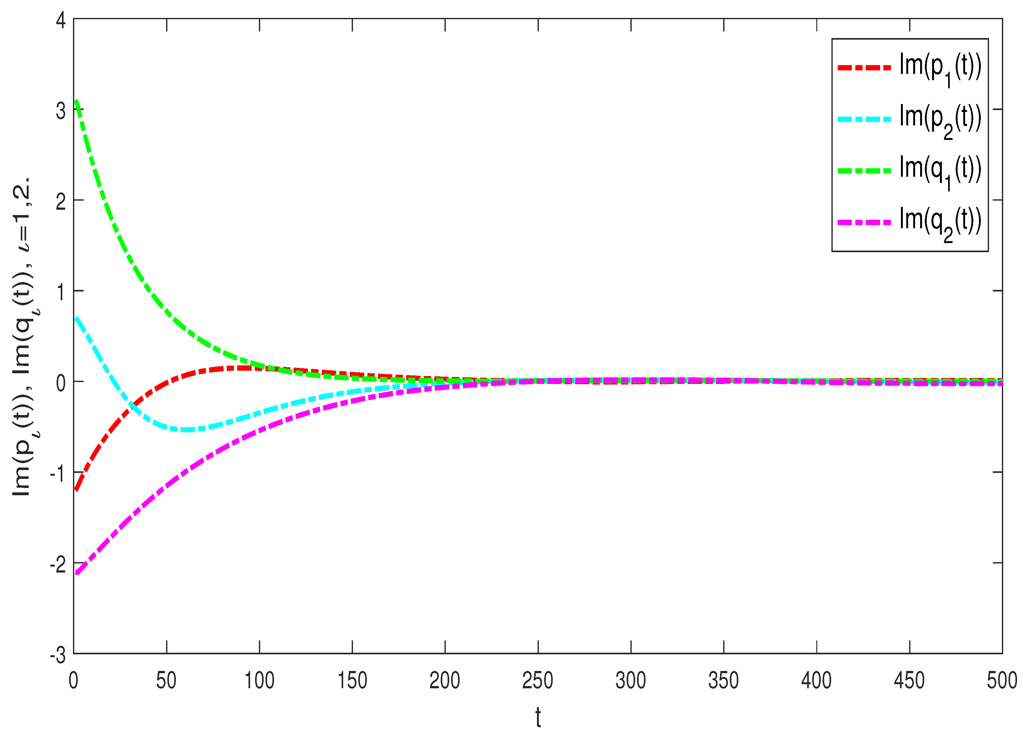
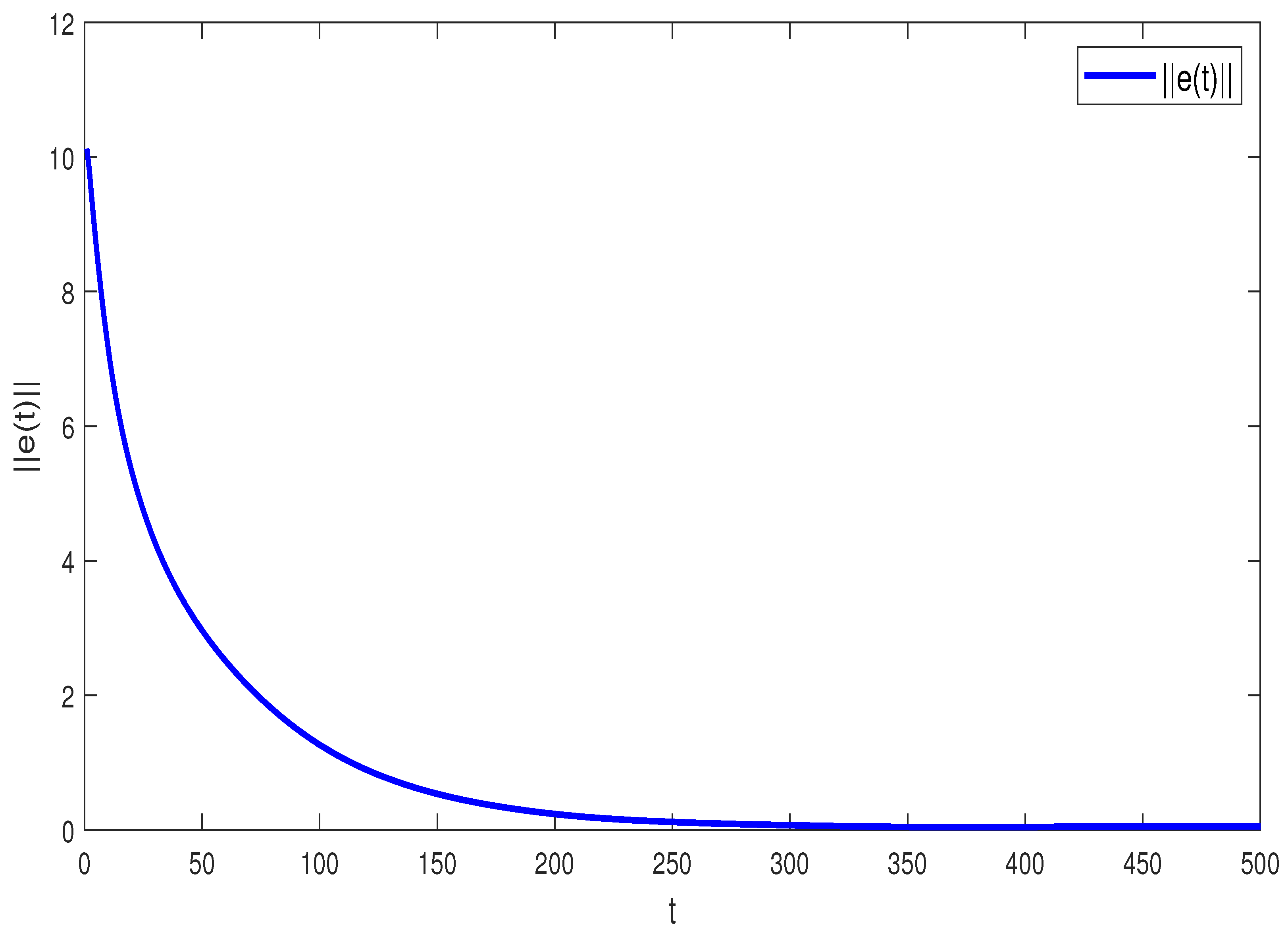
4. Numerical Simulation

In this section, a numerical example is provided to verify the effectiveness of the adaptive synchronization criterion for FOUCVCNNs.

Example 1. 

We chose the following FOUCVCNN model

$$\left\{\begin{array}{ccc}{\displaystyle { }_{t_0}^c{D}_t^{\gamma }{\alpha }_{\iota }(t)}& =\hfill & {\displaystyle -a_{\iota }{\alpha }_{\iota }(t)+\sum _{\eta =1}^2\left({\zeta }_{\iota \eta }+▵{\zeta }_{\iota \eta }(t)\right)h_{\eta }({\alpha }_{\eta }(t))+c_{\iota }{\beta }_{\iota }(t)+{\Psi }_{\iota }(t),}\hfill \\ {\displaystyle { }_{t_0}^c{D}_t^{\gamma }{\beta }_{\iota }(t)}& =\hfill & {\displaystyle -\left(b_{\iota }+▵b_{\iota }(t)\right){\beta }_{\iota }(t)+h_{\iota }({\alpha }_{\iota }(t)),\iota ,\eta =1,2,}\hfill \end{array}\right.$$

(9)

where $\gamma =0.98$, $c_1=1+i$, $c_2=1.5+i$, ${\Psi }_1(t)={\Psi }_2(t)=0$, $h_{\eta }({\alpha }_{\eta }(t))=tanh\left(\mathrm{Re}({\alpha }_{\eta }(t))\right)+itanh\left(\mathrm{Im}({\alpha }_{\eta }(t))\right)$, $a_1=4.6-i$, $a_2=3.6+2i$, $b_1=4+i$, $b_2=2.5+i$, $▵{\zeta }_{11}(t)=0.01sint-0.01sint$, $▵{\zeta }_{12}(t)=0.01cost-0.01costi$, $▵{\zeta }_{21}(t)=0.01cost+0.01costi$, $▵{\zeta }_{22}(t)=0.01sint+0.01sinti$, $▵b_1(t)=0.01cost+0.01costi$, $▵b_2(t)=0.01cost-0.01costi$, and the initial values of FOUCVCNN (9) are chosen as ${\alpha }_1(0)=0.5-0.1i$, ${\alpha }_2(0)=-0.6+0.5i$, ${\beta }_1(0)=0.5+0.1i$, ${\beta }_2(0)=0.1-0.2i$.

The controlled FOUCVCNN model is considered as

$$\left\{\begin{array}{c}{\displaystyle { }_{t_0}^c{D}_t^{\gamma }{\widehat{\alpha }}_{\iota }(t)=-a_{\iota }{\widehat{\alpha }}_{\iota }(t)+\sum _{\eta =1}^2\left({\zeta }_{\iota \eta }+▵{\zeta }_{\iota \eta }(t)\right)h_{\eta }({\widehat{\alpha }}_{\eta }(t))+c_{\iota }{\widehat{\beta }}_{\iota }(t)+{\Psi }_{\iota }(t)+u_{\iota }^{†}(t),}\hfill \\ {\displaystyle { }_{t_0}^c{D}_t^{\gamma }{\widehat{\beta }}_{\iota }(t)=-\left(b_{\iota }+▵b_{\iota }(t)\right){\widehat{\beta }}_{\iota }(t)+h_{\iota }({\widehat{\alpha }}_{\iota }(t))+u_{\iota }^{‡}(t),}\hfill \end{array}\right.$$

(10)

where $h_{\eta }({\widehat{\alpha }}_{\eta }(t))=tanh\left(\mathrm{Re}({\widehat{\alpha }}_{\eta }(t))\right)+itanh\left(\mathrm{Im}({\widehat{\alpha }}_{\eta }(t))\right)$, and the initial values of FOUCVCNN (10) are ${\widehat{\alpha }}_1(0)=1.6-1.2i$, ${\widehat{\alpha }}_2(0)=-1.2+1.2i$, ${\widehat{\beta }}_1(0)=-2.6+3.2i$, ${\widehat{\beta }}_2(0)=2.5-2.3i$. The other parameter values are consistent with those of FOUCVCNN (9).

The adaptive controller in FOUCVCNN (10) is designed to be the same as (3), setting ${\delta }_1=0.02$, ${\delta }_2=0.02$, ${\sigma }_1=0.02$, ${\sigma }_2=0.02$, ${\theta }_1(0)=0.2$, ${\theta }_2(0)=0.25$, ${\vartheta }_1(0)=0.3$, ${\vartheta }_2(0)=0.35$, $\rho =\varrho =0.015$. Based on Theorem 1, FOUCVCNNs (9) and (10) are synchronized, which is validated by Figure 1 and Figure 2. We defined the whole error norm as ${\displaystyle ||e(t)||=\sum _{\iota =1}^2|p_{\iota }(t)|+\sum _{\iota =1}^2|q_{\iota }(t)|}$, and the time evolution of $||e(t)||$ is depicted in Figure 3. The trajectories of adaptive control gains ${\theta }_{\iota }(t)$ and ${\vartheta }_{\iota }(t)$ are displayed in Figure 4.

Remark 7. 

From Figure 4, the adaptive control gains at both ${\theta }_{\iota }(t)$ and ${\vartheta }_{\iota }(t),\iota =1,2$ tend towards a positive constant, which can further illustrate the effectiveness of the synchronization criteria; this is due to the fact that the Caputo fractional derivative of any constant is zero.

5. Conclusions

In this paper, the topic of the adaptive synchronization of FOUCVCNNs has been investigated via a non-decomposition approach. By designing a new adaptive control strategy and constructing a suitable Lyapunov function, a novel adaptive synchronization criterion for FOUCVCNNs has been obtained by means of the fractional Lyapunov method and inequality techniques. Moreover, some relevant corollaries have been yielded under the simplification of the model and controller. Finally, we provided a numerical example to illustrate the validity of adaptive synchronization results. Note that the nonlinear control strategy has the advantages of being less conservative; our future research will focus on the study of nonlinear control-based synchronization for FOUCVCNNs and its practical applications.

References

1. Hu, M.; Huang, X.; Shi, Q.; Yuan, F. Design and analysis of a memristive Hopfield switching neural network and application to privacy protection. Nonlinear Dyn. 2024, 112, 12485–12505. [Google Scholar] [CrossRef]
2. Cao, J.; Stamov, F.; Stamov, G.; Stamova, I. Impulsive controllers design for the practical stability analysis of gene regulatory networks with distributed delays. Fractal Fract. 2023, 7, 847. [Google Scholar] [CrossRef]
3. Chen, D.; Zhang, Z. Finite-time synchronization for delayed BAM neural networks by the approach of the same structural functions. Chaos Solitons Fractals 2022, 164, 112655. [Google Scholar] [CrossRef]
4. Aili, A.; Chen, S.; Zhang, S. Event-triggered synchronization of coupled neural networks with reaction-diffusion terms. Mathematics 2024, 12, 1409. [Google Scholar] [CrossRef]
5. Zhang, L.; Zhu, Q.; Huang, T. Global polynomial synchronization of proportional delayed inertial neural networks. IEEE Trans. Syst. Man Cybern. Syst. 2023, 53, 4487–4497. [Google Scholar]
6. Wang, L.; Zhang, C. Exponential synchronization of memristor-based competitive neural networks with reaction-diffusions and infinite distributed delays. IEEE Trans. Neural Netw. Learn. Syst. 2024, 35, 745–758. [Google Scholar] [CrossRef] [PubMed]
7. Cohen, M.; Grossberg, S. Absolute stability of global pattern formation and parallel memory storage by competitive neural networks. IEEE Trans. Syst. Man Cybern. 1983, 13, 815–825. [Google Scholar] [CrossRef]
8. Adhira, B.; Nagamani, G. Exponentially finite-time dissipative discrete state estimator for delayed competitive neural networks via semi-discretization approach. Chaos Solitons Fractals 2023, 176, 114162. [Google Scholar] [CrossRef]
9. Xu, C.; Jiang, M.; Hu, J. Mean-square finite-time synchronization of stochastic competitive neural networks with infinite time-varying delays and reaction-diffusion terms. Commun. Nonlinear Sci. Numer. Simulat. 2023, 127, 107535. [Google Scholar] [CrossRef]
10. Wang, L.; Tan, X.; Wang, Q.; Hu, J. Multiple finite-time synchronization and settling-time estimation of delayed competitive neural networks. Neurocomputing 2023, 552, 126555. [Google Scholar] [CrossRef]
11. Yu, J.; Hu, C.; Jiang, H. Corrigendum to projective synchronization for fractional neural networks. Neural Netw. 2015, 67, 152–154. [Google Scholar] [CrossRef]
12. Chen, S.; Li, H.; Wang, L.; Hu, C.; Jiang, H.; Li, Z. Finite-time adaptive synchronization of fractional-order delayed quaternion-valued fuzzy neural networks. Nonlinear Anal. Model. Control 2023, 28, 804–823. [Google Scholar] [CrossRef]
13. Zhang, S.; Du, F.; Chen, D. New approach to quasi-synchronization of fractional-order delayed neural networks. Fractal Fract. 2023, 7, 825. [Google Scholar] [CrossRef]
14. Li, H.; Hu, C.; Cao, J.; Jiang, H.; Alsaedi, A. Quasi-projective and complete synchronization of fractional-order complex-valued neural networks with time delays. Neural Netw. 2019, 118, 102–109. [Google Scholar] [CrossRef] [PubMed]
15. Chen, S.; Li, H.; Kao, Y.; Zhang, L.; Hu, C. Finite-time stabilization of fractional-order fuzzy quaternion-valued BAM neural networks via direct quaternion approach. J. Frankl. Inst. 2021, 358, 7650–7673. [Google Scholar] [CrossRef]
16. Rajchakit, G.; Chanthorn, P.; Niezabitowski, M.; Raja, R.; Baleanu, D.; Pratap, A. Impulsive effects on stability and passivity analysis of memristor-based fractional-order competitive neural networks. Neurocomputing 2020, 417, 290–301. [Google Scholar] [CrossRef]
17. Zhang, F.; Huang, T.; Wu, Q.; Zeng, Z. Multistability of delayed fractional-order competitive neural networks. Neural Netw. 2021, 140, 325–335. [Google Scholar] [CrossRef] [PubMed]
18. Xu, Y.; Yu, J.; Li, W.; Feng, J. Global asymptotic stability of fractional-order competitive neural networks with multiple time-varying-delay links. Appl. Math. Comput. 2021, 389, 125498. [Google Scholar] [CrossRef]
19. Wu, Z.; Nie, X.; Cao, B. Coexistence and local stability of multiple equilibrium points for fractional-order state-dependent switched competitive neural networks with time-varying delays. Neural Netw. 2023, 160, 132–147. [Google Scholar] [CrossRef]
20. Pratap, A.; Raja, R.; Cao, J.; Rajchakit, G.; Fardoun, H. Stability and synchronization criteria for fractional order competitive neural networks with time delays: An asymptotic expansion of Mittag Leffler function. J. Frankl. Inst. 2019, 356, 2212–2239. [Google Scholar] [CrossRef]
21. Gao, P.; Ye, R.; Zhang, H.; Stamova, I.; Cao, J. Asymptotic stability and quantitative synchronization of fractional competitive neural networks with multiple restrictions. Math. Comput. Simul. 2024, 217, 338–353. [Google Scholar] [CrossRef]
22. Wang, S.; Jian, J. Predefined-time synchronization of incommensurate fractional-order competitive neural networks with time-varying delays. Chaos Solitons Fractals 2023, 177, 114216. [Google Scholar] [CrossRef]
23. Yang, S.; Jiang, H.; Hu, C.; Yu, J. Synchronization for fractional-order reaction-diffusion competitive neural networks with leakage and discrete delays. Neurocomputing 2021, 436, 47–57. [Google Scholar] [CrossRef]
24. Shafiya, M.; Nagamani, G.; Dafik, D. Global synchronization of uncertain fractional-order BAM neural networks with time delay via improved fractional-order integral inequality. Math. Comput. Simul. 2022, 191, 168–186. [Google Scholar] [CrossRef]
25. Chen, S.; Yang, J.; Li, Z.; Li, H.; Hu, C. New results for dynamical analysis of fractional-order gene regulatory networks with time delay and uncertain parameters. Chaos Solitons Fractals 2023, 175, 114041. [Google Scholar] [CrossRef]
26. Ali, M.S.; Hymavathi, M.; Kauser, S.; Rajchakit, G.; Hammachukiattikul, P.; Boonsatit, N. Synchronization of fractional order uncertain BAM competitive neural networks. Fractal Fract. 2022, 6, 14. [Google Scholar]
27. Li, H.; Kao, Y.; Bao, H.; Chen, Y. Uniform stability of complex-valued neural networks of fractional order with linear impulses and fixed time delays. IEEE Trans. Neural Netw. Learn. Syst. 2022, 33, 5321–5331. [Google Scholar] [CrossRef] [PubMed]
28. Panda, S.; Nagy, A.; Vijayakumar, V.; Hazarika, B. Stability analysis for complex-valued neural networks with fractional order. Chaos Solitons Fractals 2023, 175, 114045. [Google Scholar] [CrossRef]
29. Xu, D.; Tan, M. Multistability of delayed complex-valued competitive neural networks with discontinuous non-monotonic piecewise nonlinear activation functions. Commun. Nonlinear Sci. Numer. Simul. 2018, 62, 352–377. [Google Scholar] [CrossRef]
30. Zheng, B.; Hu, C.; Yu, J.; Jiang, H. Finite-time synchronization of fully complex-valued neural networks with fractional-order. Neurocomputing 2020, 373, 70–80. [Google Scholar] [CrossRef]
31. Cheng, J.; Zhang, H.; Zhang, W.; Zhang, H. Quasi-projective synchronization for Caputo type fractional-order complex-valued neural networks with mixed delays. Int. J. Control Autom. 2022, 20, 1723–1734. [Google Scholar] [CrossRef]
32. Xu, Y.; Li, H.; Yang, J.; Zhang, L. Quasi-projective synchronization of discrete-time fractional-order complex-valued BAM fuzzy neural networks via quantized control. Fractal Fract. 2024, 8, 263. [Google Scholar] [CrossRef]
33. Chen, S.; Li, H.; Bao, H.; Zhang, L.; Jiang, H.; Li, Z. Global Mittag-Leffler stability and synchronization of discrete-time fractional-order delayed quaternion-valued neural networks. Neurocomputing 2022, 511, 290–298. [Google Scholar] [CrossRef]
34. Hu, X.; Wang, L.; Zhang, C.; Wan, X.; He, Y. Fixed-time stabilization of discontinuous spatiotemporal neural networks with time-varying coefficients via aperiodically switching control. Sci. China Inf. Sci. 2023, 66, 152204. [Google Scholar] [CrossRef]
35. Zhu, S.; Lü, J. Further on pinning synchronization of dynamical networks with coupling delay. SAIM J. Control Optim. 2024, 62, 1933–1952. [Google Scholar] [CrossRef]
36. Kilbas, A.; Srivastava, H.; Trujillo, J. Theory and Application of Fractional Differential Equations; Elsevier: New York, NY, USA, 2006. [Google Scholar]
37. Podlubny, I. Fractional Differential Equations; Academic Press: San Diego, CA, USA, 1999. [Google Scholar]
38. Xu, C.; Liao, M.; Wang, C.; Sun, J.; Lin, H. Memristive competitive hopfield neural network for image segmentation application. Cogn. Neurodynamics 2023, 17, 1061–1077. [Google Scholar] [CrossRef]
39. Zhang, F.; Huang, T.; Wu, A.; Zeng, Z. Mittag-Leffler stability and application of delayed fractional-order competitive neural networks. Neural Netw. 2024, 179, 106501. [Google Scholar] [CrossRef]
Figure 1. The real part of synchronization error of FOUCVCNNs (9) and (10) under adaptive controller (3).
Fractalfract 08 00449 g001
Figure 2. The imaginary parts of the synchronization errors in FOUCVCNNs (9) and (10) under adaptive controller (3).
Fractalfract 08 00449 g002
Figure 3. The whole synchronization error norm of FOUCVCNNs (9) and (10) under adaptive controller (3).
Fractalfract 08 00449 g003
Figure 4. The state trajectories of adaptive control gains θ ι ( t ) and ϑ ι ( t ) in adaptive controller (3).
Fractalfract 08 00449 g004
Disclaimer/Publisher’s Note: The statements, opinions and data contained in all publications are solely those of the individual author(s) and contributor(s) and not of MDPI and/or the editor(s). MDPI and/or the editor(s) disclaim responsibility for any injury to people or property resulting from any ideas, methods, instructions or products referred to in the content.